Numerical Modelling in a Multi-Scale Ocean - Bitly

Numerical Modelling in a Multi-Scale Ocean

D. B. Haidvogel, Rutgers University E. N. Cuchitser, Rutgers University S. Danilov, Alfred Wegener Institute B. Fox-Kemper, Brown University

ABSTRACT Systematic improvement in ocean modelling and prediction systems over the past several decades has resulted from several concurrent factors. The first of these has been a sustained increase in computational power, as summarized in Moore’s Law, without which much of this recent progress would not have been possible. Despite the limits imposed by existing computer hardware, however, significant accruals in system performance over the years have been achieved through novel innovations in system software, specifically the equations used to represent the temporal evolution of the oceanic state as well as the numerical solution procedures employed to solve them.

Here, we review several recent approaches to system design that extend our capability to deal accurately with the multiple time and space scales characteristic of oceanic motion. The first two are methods designed to allow flexible and affordable enhancement in spatial resolution within targeted regions, relying on either a set of nested structured grids or alternatively a single unstructured grid. Finally, spatial discretization of the continuous equations necessarily omits finer, sub-gridscale processes whose effects on the resolved scales of motion cannot be neglected. We conclude with a discussion of the possibility of introducing sub-gridscale parameterizations to reflect the influences of unresolved processes.

Keywords: Ocean modelling, nested grids, finite element and volume methods, sub-gridscale parameterization

1

1. Introduction The equations of motion for the ocean cannot be solved exactly except under highly idealized conditions. This is so for several reasons. First, the equations governing the dynamics of the open ocean in their exact form are nonlinear partial differential equations for which analytic, closedform solutions are unobtainable. Even were this not the case, many if not all of the environmental fields needed to specify a given problem --- bathymetry, coastline geometry, surface forcing, initial and boundary conditions, etc. --- are non-analytic fields determined from observations; these in turn are uncertain to within observational error and often non-uniformly distributed in space and time. As a consequence of these restrictions, solutions to the equations of motion, unless greatly simplified, must be determined numerically via approximate solution procedures. Obtaining predictions of future states in the ocean therefore raises several related, and often competing, issues. These include: first, how to discretize the continuous equations of motion and their component variables (and what potential sources of error may be introduced thereby). Of particular recent interest, given the broad range of scales relevant to ocean prediction (e.g., global, regional, coastal, estuarine, etc.), are multi-scale discretization techniques that allow timely and affordable predictions. Second, because discretization necessarily omits some smaller-scale processes, the inclusion of the effects of sub-gridscale influences via appropriate parameterizations must be considered. In what follows, we first discuss some general properties and consequences of the numerical solution of the oceanic equations of motion. We next briefly review two methodologies used to extend the range of spatial scales covered by such solutions, namely the use of nested structured grids and unstructured grids, respectively. Finally, we close with a discussion of the “scale-aware” parameterization of sub-gridscale processes. 2

2. A brief introduction to ocean numerical modelling: issues, techniques and consequences Ocean processes cover an enormous range of space and time scales; some examples are shown schematically in Figure 1. Notwithstanding this complexity, the equations governing the time evolution of oceanic processes are for the most part well understood. The primitive equations which form the basis for many ocean circulation prediction systems are derived from the conservation laws for mass, momentum (Newton’s Law, F=ma), heat (the First Law of Thermodynamics) and tracers (e.g., salinity), supplemented with an equation of state relating the density of the ocean to in situ properties (temperature, salinity, pressure).

The primary

assumptions made along the way are the Boussinesq and hydrostatic approximations.

The

derivation and implications of the primitive equations are reviewed in the companion contribution by Jacobs and Fox-Kemper (2017). In their “simplest” form, the primitive equation set incorporates seven non-linear partial differential equations (PDE) describing the space/time evolution of the seven primary oceanic variables: velocity components in three space dimensions (u, v, w), temperature and salinity, density and pressure. In addition to conservation of mass, momentum and heat upon which they are based, the primitive equation set has many additional desirable properties, among them conservation of higher-order quantities such as energy, vorticity and enstrophy (vorticity squared). Although we will not dwell overly long on the (very important) issue of computational efficiency, it is to be noted that the hydrostatic primitive equations encompass processes of both hyperbolic (wave) and parabolic (diffusion) types, but avoid the elliptic character of the equation set in the absence of the hydrostatic approximation. This yields great computational savings in that solutions of elliptic equations are not required. However, in exchange for this economy, the 3

solution of the primitive equations requires some “regularization” (smoothing) if convergence under grid refinement is to be guaranteed (see, e.g., Vitousek and Fringer 2011).

Figure 1: Space-time scales of some oceanic processes. The latitude has been set to 25o N. The characteristic length scale of water bodies is taken to be sqrt(area).

The essence of determining approximate solutions to the equations of motion is the representation of each of the four-dimensional dependent variables – velocity for instance – as a discrete function described by a finite set of numbers, rather than as a continuous function of space and time, i.e., u(x, y, z, t). As is clear, this representation requires specific methodologies for discretization of the four independent variables. After discretization in space and time, the resulting approximate difference equations (ADE), supplemented with an appropriate set of initial and boundary conditions, are solved to obtain solutions representing future ocean states. The primitive equations are essentially “exact” for processes for which the hydrostatic and Boussinesq approximations are appropriate (i.e., the upper-right quadrant of Fig. 1) as well as 4

conservative of the properties noted above.

However, solutions to the ADE are clearly

approximate only, and several questions therefore arise. These include: in what way(s) do errors arise, how big are they, and how may they be minimized and/or avoided; do solutions to the ADE converge to the exact solution as discretization intervals in space/time are reduced; and can the conservation of properties displayed in the original exact equations be maintained in the ADE despite inevitable error? We discuss these questions, by example, next. To do so, we will use a convenient, reduced form of the equations of motion, namely the linearized shallow water equations that apply to a single, shallow layer of constant density. Treatment of ocean stratification will be discussed below. In the absence of density variation, and with the inclusion of a conserved tracer field, the reduced equation set is as follows: u u  U  fv   g  K  2u t x x v v  U  fu   g  K  2v t x y  u v  H(  )  0 t x y T T U  K  2T t x

where the dependent variables are: (u,v), the horizontal velocity components in the x and y coordinate directions respectively; η, the elevation of the sea surface above its resting position; and T, a tracer field. The parameters appearing in the equations, assumed constant, include: U, an advecting zonal velocity; f, the Coriolis parameter; g, the acceleration of gravity; H, the resting layer depth; and K, a horizontal mixing coefficient.

5

a. Spatial differencing: Taylor series and a simple geostrophic example Spatial discretization of the dependent variables and spatial operators in the equations of motion can be approached in several ways. The methods most commonly employed in ocean modelling are the finite difference, finite volume, and finite element methods. 1 We will use the first of these techniques here to illustrate some general principals and results. The implementation of the latter two methods is discussed below. The finite difference (FD) method assumes that each dependent variable, say u(x,y,z,t), i s defined by its values at a finite number of spatial points (xj, yk, zl) where j, k and l are integer subscripts. Typically, these “grid points” form a structured grid and are uniformly spaced, although some degree of non-uniform spatial resolution can be accommodated with appropriate coordinate transformations (Thompson et al. 1982). For simplicity, consider the function u(x,t) in one space dimension, and suppose that we seek approximate forms for the partial derivatives ∂ x, ∂x2, etc. along with an estimate of the error incurred by the approximation. Consider a set of equally spaced grid points (xj = jΔx) and an associated set of values u(xj) ≡ uj. Finite difference approximations to differential equations can be obtained in several ways. The most often used is the Taylor series method. The Taylor series expansions for the behavior of a smooth function about a central point xj are u ( x j  x)  u ( x j )  (x)u   (

x 2 x3 )u   ( )u   O(x 4 ) 2 3!

x 2 x3 u ( x j  x)  u ( x j )  (x)u  ( )u  ( )u  O(x 4 ) 2 3!

1

Other spatial representation methods based upon higher-order expansions in continuous Fourier or polynomial basis functions, while enjoying a lengthy history in atmospheric prediction, have seen more limited use in ocean modelling. See, e.g., Wunsch et al. (1997) and Choi et al. (2004).

6

where the prime notation designates a partial derivative (i.e., u ≡ ∂xu). By combining these expressions, a variety of FD approximations may be derived, including u( x j ) 

u( x j ) 

u ( x j  x)  u ( x) x

 O(x)

u ( x j  x)  u ( x j  x) 2x

 O(x 2 )

and

u( x j ) 

u ( x j  x)  2u( x j )  u( x j  x) x

2

 O(x 2 ) .

Here O(Δx) and O(Δx2) represent residual (error) terms proportional to Δx and Δx2 respectively, and indicate the rate at which the error made by the approximation may be reduced as the grid spacing Δx is refined. An approximation whose leading-order error term is proportional to Δx is referred to as “first-order” in space; for an error term proportional to Δx2 the approximation is said to be of “second-order”. Higher-order approximations may be obtained by using additional gridpoint values (e.g., u(xj ± 2Δx)). As the first two expressions illustrate, finite difference approximations can be constructed in alternate ways, each having their own distinct error properties. Note that centered FD approximations (those using gridpoint values set equally to either side of the central point) are generally more accurate than one-sided approximations (those using sets of values asymmetrically distributed to one side or the other). As a first example, consider geostrophic currents in the ocean. At lowest order in a Rossby number expansion, the open ocean is in quasi-steady hydrostatic and geostrophic balance. From the first of our equations above, north-south geostrophic flow near the ocean surface is given by 7

fv  g

 (see, e.g., Stewart 2008). Let us suppose that the sea surface perturbation is oscillatory x

in space  ( x)  0eikx , where η0 is the amplitude and k the wavenumber (2π / wavelength) of the sea surface disturbance. From this, the north-south component of geostrophic flow is found to be exactly v  (0 g / f )ikeikx . It is instructive to ask what geostrophic flow we would obtain if we were to adopt a centered, second-order approximation to the term

 on a FD grid of spacing Δx. In this case, x

we assume:   0  eik ( x x )  eik ( x x )  / 2x x

from which, after substitution and a bit of manipulation, we obtain v  (0 g / f )ikeikx  sin(k x) / k x  .

Our FD approximation matches the exact result except for an additional factor of (sin(kΔx)/kΔx). The error in utilizing our centered, second-order approximation is therefore determined by the departure of this additional multiplicative factor from a value of unity. Note that the FD result may be written v  (0 g / f )ik eikx where the modified wavenumber k   k sin(k x) / k x (see, e.g., Moin 2010). Because k  is real, the central differencing operator is seen in this case to produce no phase error, as it would if k  had an imaginary component. On a uniform FD grid, the admissible wavenumbers k range from ~0 (very fine resolution relative to the wavelength of η) to a value of (π/Δx). The latter limit applies because the finest perturbation resolvable on a grid of spacing Δx has a wavelength of 2Δx. As (2π/kΔx) is equal to

8

the number of grid points per wavelength of η, we can compute the percent error in our approximation as a function of grid point resolution. The result is shown in Figure 2.

Figure 2: Percent error in the value of surface geostrophic current when a second-order FD approximation is used to evaluate the surface pressure gradient on a uniform grid.

Several features in Figure 2 are of interest. Suppose that we wanted to guarantee an error less than 5%. For this discretization and the assumed form of the sea surface perturbation, we would require roughly 12 grid points per wavelength of the significant sea surface undulations. At reduced resolution, say 6 points per wavelength, we are already up to roughly 20% error. Finally, for the finest resolvable sea surface perturbation, the 2Δx wave, the error is 100%; there is no geostrophic flow at all at this scale despite the fact that the 2Δx wave has, in the continuum, the most rapid spatial variation.

9

b. Horizontal discretization in two dimensions: propagating waves on staggered grids Thus far we have assumed that all variables are available on a common set of horizontal grid points.

Such an arrangement is not necessary however.

An alternative is the use of

horizontally staggered grids in which the dependent variables are offset from each other in various ways. Five examples of horizontal staggering, the so-called Arakawa “A”, “B”, “C”, “D” and “E” grids (Arakawa 1966), are shown in Figure 3. Historically, the most widely used arrangements of variables for finite difference primitive equation ocean models have been the B and C grids; however, the majority of models in widespread current use have adopted the C grid. The arrangement of variables on the C grid places the discrete values of the sea surface height and tracer fields at the center of each grid cell, and the values of the u and v velocity components on the cell edges in the sense of normally directed flow (Fig. 3). Consider the impact on processes resulting from the discretization of their governing equations on a C grid. We first return briefly to the geostrophic example above. Note that the arrangement of variables on the C grid facilitates the discretization of the surface pressure gradient terms in the equations for geostrophic balance. Because of the positioning of the values of η, the sea surface gradient terms needed at u and v grid points can both be obtained from central differences across a single Δx or Δy. (On our non-staggered example above, the central difference was obtained across 2Δx.) For second-order differencing, an error reduction of a factor of four is realized on the staggered C grid. A broad space-time spectrum of propagating waves exists within the ocean and can be associated with gravitational, planetary and/or topographic restoring forces (see, e.g., Pedlosky 2003). Two classes of wave motions which are intimately involved in basin-scale adjustment are inertia-gravity waves, which mediate gravitational adjustment, and planetary or Rossby waves, 10

which are the primary basin-wide agents of geostrophic adjustment. Systematic errors in the representation of these wave processes have consequences for the manner in which numerical ocean circulation models respond to time-varying forcing.

Figure 3: The arrangement of variables on the Arakawa grids.

As a second example, consider our shallow water equation set under the assumption of no large-scale advection (U=0) or diffusion (K=0).

 (

Defining the horizontal divergence

u v  ) , the equations for (u, v, η) can be combined to form the hyperbolic equation for the x y

propagation of inertia-gravity waves:

 2  ( f 2  gH  2 )  0 . 2 t 11

i ( kx  ly t ) The insertion of a trial wave solution proportional to e into this equation yields the exact

dispersion relation for inertia-gravity waves:

 ( )2  1  Rd2 (k 2  l 2 ) f where Rd  gH / f is the Rossby deformation radius. As we have noted, on a C grid the discretized form of the surface pressure gradient terms are easily obtained by a central difference across a single grid interval (Δx or Δy). However, the discretized forms of the Coriolis terms (requiring fv at a u point, and fu at a v location) each requires a four-way average of v and u values, respectively. This is in contrast to a non-staggered grid or the Arakawa B grid, neither of which would require spatial averaging to specify a centered estimate of the Coriolis terms. For a propagating, wave-like solution of the form e

i ( kx  ly t )

, the effect of spatial

differencing on the estimates of the surface pressure gradient terms follows from the geostrophic example above, yielding multiplicative terms proportional to sin(

k x l y ) and sin( ) in the 2 2

respective momentum equations. In contrast, the effects of the spatial averaging on the Coriolis terms can be shown to result in factors of cos(

k x l y ) and cos( ) for averaging in x and y. 2 2

Taking a uniform grid (Δx=Δy) for convenience, and for the moment assuming exact time differencing, the corresponding form for the dispersion relation on a C grid becomes:

R   k x l x k x l x  ( )2  cos2 ( ) cos 2 ( )  4( d )2 sin 2 ( )  sin 2 ( )  . f 2 2 x  2 2 

12

The departure of the approximate dispersion relation (ADR) from its exact form is found to be dependent on the two non-dimensional parameters (

l x k x ) and ( ); these are (π times) the ratio 2 2

of the grid spacing to the wavelength of the wave in the x and y directions. Recalling that k and l are, respectively, 2π divided by the x and y wavelengths of the wave, and that the finest resolvable wavelength is 2Δx, these “error parameters” range in value from near zero (the limit of very fine

 resolution of the wave) to ( ) . From this it is clear that the ADR approaches the exact form in 2 the limit (Δx0)2. The maximum error incurred on the C grid occurs for the most poorly resolved wave (k  l 

 x

) , for which:

 4 ( )2  0  [( 2 ) Rd2 (k 2  l 2 )]k l  / x f  where the “0” has been included to emphasize that the contribution to the ADR from the Coriolis parameter has disappeared entirely. In addition, the contribution to the ADR from the gravity waves has been reduced by a factor of π2. In other words, the phase speed (c ph 

 k

) of the gravity

waves has been reduced by a factor of π. Note that, in the continuum, pure gravity waves are nondispersive, that is, their phase speed is constant, independent of wavenumber. However, when produced on a C grid, they are dispersive. In the preceding semi-discrete example (discrete in space, exact in time) the bi-directional wave (hyperbolic) character of the solutions is maintained, albeit with errors in the phase speed

2

Note that sin(kΔx/2)(kΔx/2) and cos(kΔx/2)1 as Δx0.

13

dependent on wavenumber.

This fortuitous outcome is a consequence of the symmetric

differencing and averaging operations defined on the C grid, which do not change the character of the resulting ADE. Further discussion of the influence of staggered grids on the propagation of geophysical waves can be found in Wajsowicz (1986) and Dukowicz (1995).

c. Time marching of the wave equation: Mix and match So far, so good. However, numerical solution of the equations of motion requires that they be discretized in time as well as in space. That is, approximate forms for the time derivative must be specified that relate the future values of the dependent variables to their past values. As with approximations in space, there are many approaches to time differencing. A thorough discussion of time differencing is beyond the scope here. Instead, we will use several simple time-marching schemes to support our general remarks. The reader is directed to the more comprehensive discussions in (e.g.) Durran (1999).

Consider the generic tracer equation

T  F (T ) where F is a linear function describing the t

time-evolution of T, e.g., the advection, diffusion, or combined advection-diffusion equations. As in space, we divide the continuous time interval into discrete increments, or time steps, Δt. Then integration of the tracer equation in time yields a relationship between past and future values of the prognostic variable, i.e., a time-marching scheme. Time integration may in principle be performed over any number of past time levels. In practice, integration from t0 to t0+Δt (a “onestep” scheme) or from t0-Δt to t0+Δt (a “two-step” scheme) are typically employed. Several simple one- and two-step time-marching schemes can be written in the following form: T(n+1) = αT(n) + βT(n-1) + Δt{γF(n+1) + κF(n) + εF(n-1)}. Here, α-ε are constants, and the 14

superscript notation denotes the time step (i.e., T(n)≡T(x, nΔt)). It has been assumed that values of T are available at a minimum of two prior time levels. Simple time-marching schemes that fit this description include: Euler forward (α=1, κ=1; β=γ=ε=0), Euler backward (α=1, γ=1), trapezoidal (α=1, γ=κ=1/2), leapfrog (β=1, κ=2) and Adams-Bashforth (α=1, κ=3/2, ε=-1/2). From our discussion of differencing in space, it may be anticipated that time differences that are “centered” – that is, with the estimate of F centered within the interval spanned by the time steps of T -- will be more accurate than those that are not. This is indeed the case. Of our five simple time-marching schemes, the two Euler methods are of first order in time. The remaining three, including the well-known leapfrog scheme, are centered in this sense and consequently of second order. Note that higher-order accuracy can be obtained with either a one- or two-step scheme. In general, two types of error may arise in solutions to the ADE. The first, dispersive error, we have already encountered. The second is amplitude error, in which the magnitude of the approximate solution differs from its exact counterpart. A particularly unfortunate situation arises when the time-marching scheme allows the approximate solution to grow in amplitude without limit, rather than behave stably as in the propagating wave example above wherein the amplitude of the wave is preserved in time. This is termed numerical instability and caution is always needed to avoid an approximate solution that “blows up”. In reference above to the semi-discrete, bi-directional wave equation, we have noted that it is helpful for the ADE to preserve the character – in this instance hyperbolic -- of the exact equation set. As we will see below, this is not the case for all time-marching schemes. One that does so here, however, is the following:

15

 ( n 1)   ( n ) u ( n ) v ( n ) ( )  H (  ) t x y u ( n 1)  u ( n ) v ( n 1)  v ( n )  ) f( )  g ( )( n 1) t 2 x ( n 1) (n) ( n 1) (n) v v u n  ( )f( )  g ( )( n 1) t 2 y

(

wherein a mixture of Euler forward, Euler backward and trapezoidal treatments are all used in combination. This treatment seems strange at first sight; however, manipulation of the ADE for (u, v, η) yields the equivalent ADE for horizontal divergence, namely:

(

( n 1)  ( n1)  2 ( n )   ( n1)  2 ( n )   ( n1) 2  )   f ( )  gH 2 ( n ) . 2 t 4

Here, we have left the spatial derivatives in their continuous form for convenience only; in the fully discrete ADE they would need to be approximated using symmetric averages and differences as in the C-grid examples shown above. The result of our time-marching treatments in this case is a second-order (in time and space) bi-directional wave equation in which there arises both a centered time differencing term on the left-hand side of the equation, as well as a centered time-averaging term on the right. Insertion of our trial wave equation, as above, shows that the former yields a multiplicative factor of [4sin 2 (

t 2

) / t 2 ] and the latter a factor of cos 2 (

t 2

) . It is easily verified that the solution to

the ADE approaches that of the exact equation as the time step is refined. A more complete analysis of the propagation of inertia-gravity waves for forward-backward time-differencing on staggered grids is offered by Beckers and Deleersnijder (1993).

16

d. Time-marching of the advection equation: constraints on Δt In the preceding example, a well-chosen combination of space and time discretizations reproduces the essential character of the exact equation set. In particular, the solutions to the ADE are propagating waves (whose phase speeds may however differ from the continuum result) but whose amplitudes are preserved. An alternate way to state this is to observe that the approximate dispersion relation has solutions for ω that are real numbers.

This favorable property is a

consequence of a clever choice of time marching in which implicit time weighting of the right hand-side terms (i.e., the Euler backward and trapezoidal treatments) are employed. Unfortunately, in a general setting such forward-in-time treatments may require considerable extra effort in the solution of the resulting coupled ADE. For this reason, explicitin-time marching schemes are generally preferred. In turn for the computational simplicity and efficiency that are thus gained, however, numerical instability (unbounded growth of the approximate solutions) may be encountered. It is therefore necessary to guarantee that the solution to our ADE converge to the true solution under space/time grid refinement. Two properties of an approximation are related to its convergence. These are consistency of the ADE with the original PDE, and the numerical stability of its solution. The Lax-Richtmyer equivalence theorem prescribes the relationship between convergence, consistency and stability. The theorem states for linear constant-coefficient partial differential equations that consistency plus stability together guarantee convergence. The Von Neumann method for establishing the stability of a difference approximation is the most frequently used and readily applied stability analysis method, though it is not directly applicable to nonlinear equations. In it, we test the stability of a single spatial harmonic of the

17

approximated equation. Stability of all admissible harmonics then becomes the necessary condition for stability of the overall scheme. The procedure is as follows: assume a separation of space/time variables can be made such that u(n) = λneikx, where k is the wavenumber (2π/wavelength) of the trial solution, and λ is a (possibly complex) factor specifying the phase and amplitude change in the solution from one time step to the next. Substitute the trial solution into the difference equation, and solve for λ. Then, requiring |λ| ≤ 1 – that is, precluding systematic amplitude growth -- ensures stability. As a next example, set β=ε=0 in the simple time-marching schemes from above. The resulting two-step scheme uses time levels n and (n+1) only. Then, for the advection equation T T U  0 , and for exact spatial differencing, the Von Neumann method can be applied to t x

show that 1  i   1   2  i    2 2  1  i   1    



where ϖ = UkΔt. (Note that κ+γ=1 for consistency with the original equation.) Taking the modulus of λ for the various combinations of κ and γ shows the Euler forward scheme to be unstable (|λ| = (1 + ϖ2)1/2), the Euler backward scheme to be stable but damping (|λ| = (1 + ϖ2)-1/2), and the trapezoidal scheme to be amplitude-preserving (|λ| = 1). Of these schemes, the timeimplicit trapezoidal is best (i.e., unconditionally stable and also of higher order in time) although possibly more costly to implement in a more general setting. The result of this stability analysis may be anticipated by inspection of the leading-order error terms in the ADE. Note that, from the Taylor series above:

18

T ( n1)  T ( n ) T t  2T (   ...)( n ) 2 t t 2 t  ( n1)  T t 2  2T T  (T  t   ...)( n ) . 2 x x t 2 t Combining these leading-order terms with the exact advection equation leads us to the following for the Euler-backward method applied at time step “n”:

T T U 2 t  2T U ( ) t x 2 x 2 where the higher-order terms have been dropped. The ADE with Euler-backward marching thus resembles the original advection equation but with the addition of a spurious diffusion term; after discretization, the modified equivalent PDE is no longer a simple advection equation, but rather has a combined advective-diffusive character. Note that in this case the erroneous diffusive

U 2 t coefficient ( ) is positive; hence its influence is to damp the amplitude of the solution, 2 anticipating the results of the Von Neumann stability analysis. If we had selected the Euler-forward method, the diffusive term would again enter but with a negative sign, corresponding to spurious anti-diffusion (growth) of the solution. This is again consistent with the conclusion drawn above that Euler-forward is unstable in this setting. Finally, a similar derivation for the leading-order influence of trapezoidal marching confirms that the error is dispersive, not diffusive. For the 3-step schemes (leapfrog and Adams-Bashforth), the identical Von Neumann analysis can be performed. In these cases, the result is a quadratic equation for λ, which may be solved in the usual fashion for the two associated values of λ. For leapfrog (β=1, κ=2), the two roots are 19

1  i  (1   2 )1/2 2  i  (1   2 )1/2 . The 3-step leapfrog approximation to the wave equation has two possible solutions, and both are conditionally stable, as discussed below. But by taking the limit as Δt→0, we note that the former corresponds to the true solution (λ 1→1) while the latter is unphysical (λ 2→-1). These are the physical and computational modes, respectively. The latter can be problematic if it grows too large relative to the physical mode, and hybrid schemes have been devised to keep the computational mode in check (most simply, the occasional use of a trapezoidal correction step). Finally, if we wish to assure stability of the physical mode (|λ 1| ≤ 1), then ϖ2 must be less than or equal to 1; this in turn requires UkΔt ≤ 1. The most severe restriction on Δt occurs for the largest permissible value of the wavenumber k, that is, the finest possible resolved spatial scale. The finest resolvable wavelength is 2Δx; hence kmax is (2π/2Δx) or (π/Δx) and (UΔt/Δx) ≤ (1/π). More generally, were we to discretize in space as well as time using, say, centered differences, stability would require (UΔt/Δx) ≤ 1. This is the well-known “CFL” condition for the secondorder FD approximation to the advection equation. Finally, note that Uk t  (k x)(

U t ) , the x

product of the ratio of grid spacing to wavelength and the Courant number. The latter is the ratio of the time step to the shortest advective time scale (Δx/U). The central lesson conveyed in the CFL condition is that, generally speaking, time steps are constrained by the rate at which “information” passes across the spatial grid. For the wave equation, and the second-order methods employed here, the requirement is Δt ≤ (Δx/U). With this

T  2T  K lesson in mind for the diffusion equation , simple dimensional analysis suggests that t x 2 20

the time step should be limited by a value proportional to (Δx2/K). A detailed stability analysis proves this to be the case. e. Phase errors and the creation of false extrema As our simple examples from the advection and bi-directional wave equations demonstrate, solutions obtained by approximating the time and/or space derivatives will generally not preserve the non-dispersive character of the true solution for simple gravity waves.

Instead, the

approximate solution will in general display a phase speed error that depends on the wavenumber k (and l, if in two horizontal dimensions).

This result holds even for otherwise attractive and

robust time-marching schemes such as the trapezoidal method. The dependence of phase speed error on wavenumber can have significant consequences. Consider uniform advection of a tracer field with an initial distribution that is localized in space. The localized distribution can be thought of as being made up of an overlapping sum of waves of different wavenumbers, adding up in just the right way and moving together in phase. When advanced in the continuum according to the 1d advection equation, the initial distribution is carried along at speed U without change of shape. However, an approximate solution will suffer gradual de-phasing of the component wavenumber contributions with a variety of unpleasant consequences including the potential production of false extrema (e.g., negative values) in the tracer field. A variety of approaches that attempt to minimize the consequences of dispersive errors have been explored (e.g., Zalesak 1979; Thurbin 1990; Friedrich 1998). f. Discretization in the “vertical” A significant choice in the character of numerical ocean models has been the choice of vertical discretization. In the vertical direction, the ocean has two impermeable boundaries: The

21

free surface, which is time- and space-dependent, and the bottom topography, which is usually assumed to be static except when studying near-shore sediment transport processes. The depth of the ocean floor has a significant range from the near-shore shelves at a few meters depth (even vanishing if storm surge and/or tidal wetting/drying are considered) to the deep ocean, reaching over 4,000 meters. Features such as canyons, trenches, sills and seamounts are known to impose dynamical signatures in the ocean circulation, and therefore must be properly represented. Hence, the variable ocean depth, the time-evolving free surface, as well as the space/time dependent internal density structure, are all considerations in the treatment of the vertical coordinate. Historically, ocean models were originally developed tailored to a specific vertical coordinate - e.g., geopotential, terrain-following, or isopycnal – chosen with the intended application in mind. Consider a general vertical coordinate s(i,j,k,t). Then these historically popular formulations are given by s = z (geopotential), s = z/(H + η) (terrain-following or “sigma”), and s = ρ (isopycnal). More recently in ocean models, the discretization of the vertical direction has been posed as an Arbitrary Lagrangian-Eulerian (ALE) coordinate, as originally described by Hirt et al. (1974) generally and by Bleck (2002) for the ocean. ALE can be configured to be purely Lagrangian (with no transport across the coordinate lines and a grid which moves exactly with the flow), Eulerian (wherein the fluid properties are regridded to a fixed coordinate), or anything in between (White et al. 2009). A general implementation consists of a Lagrangian step followed by a regridding of the time-dependent vertical coordinate and an Eulerian step used to compute the vertical advection relative to the moving vertical coordinate. ALE can be configured to be any of the traditional methods used in ocean models—geopotential, terrain-following or isoopycnal. Recent examples in ocean modelling are given in Chassignet et al. (2006) and Leclair et al. (2011). 22

g. Exact conservation: Yes and No A brief comment on conservation is in order. The exact equations are predicated on the conservation of properties such as mass, momentum and heat, and imply the conservation of higher-order quantities such as energy and vorticity. If the ADE are derived via consistent differencing from the exact equations expressed in flux form, then exact conservation (to within machine round-off error) can generally be guaranteed for the lowest-order conserved properties. Note however that the corresponding ADE for higher-order properties (e.g., kinetic energy, KE) may not conserve such properties exactly. For illustration, consider the derivation of the conservation statement for KE from the 1d advection equation

u(

u u  u2  u2 U )  ( ) U ( )  0 t x t 2 x 2

where the straightforward outcome in the continuum is an equivalent expression for advection of KE (

u2 in this 1d example). 2

A similar manipulation of the ADE will depart from strict

conservation via the appearance of space and time differencing error terms. These can be reduced in size by appropriate choice of space and time steps and differencing schemes. In general, however, departures from strict conservation of higher-order invariants will remain unless more complex, specialized differencing treatments are employed. h. Initial conditions, boundary conditions, and forcing functions Solution of the ADE requires the specification of initial conditions for all prognostic variables3 as well as boundary conditions at surface, bottom, sidewalls and on any open boundary

3

Recall that initial conditions may be required at more than one prior time level, depending on the nature of the time marching algorithm.

23

segments. At solid boundaries, the condition of vanishing normal flow must be imposed; beyond that, however, boundary conditions become less clear-cut. In principle, the rate and manner by which fluxes of momentum, heat, and tracers are carried across all bounding surfaces must be specified. In some cases, such fluxes may be assumed to vanish (e.g., no heat flux through an assumed insulating bottom boundary).

More generally, however, specification of boundary

mixing and fluxes becomes a question of parameterization (e.g., mixing and exchange at the ocean surface). Finally, on open boundaries the exchange of properties must also be specified (requiring a different form of parameterization). These topics are discussed further below. Note a common feature of the need to provide initial, boundary and forcing information: in any realistic application, all three require access to observational datasets of various types (atmospheric, oceanic, hydrospheric, etc.) and the quality of such datasets will determine to a large extent the success of the simulation. With the increasing use of data assimilation methodologies to improve simulation accuracy, the need for high-quality observational products becomes particularly acute. Other contributions to this volume discuss some of these topics (e.g., Brink and Kirincich 2017; Lermusiaux 2017a,b).

i. Beyond simple equations The systems of equations applied in ocean prediction are of course much more complex than the simple examples used for illustration here. Importantly, they incorporate multiple space dimensions and a simultaneous mix of interacting processes on a wide range of space/time scales. Notwithstanding this additional complexity, and the availability of a wide variety of alternate spatial and temporal discretization methods, the general messages conveyed by these simple examples continue to apply: namely, first, that insufficient spatial resolution can produce 24

significant qualitative and quantitative error; second, that discretization may alter the fundamental character of the equation set; and lastly, that time steps are typically limited by the rates of information flow across the discrete grid. The details will of course matter in each instance, and conclusions drawn in a simple setting may be overly simplistic or misleading in a more complex situation. For instance, in a multidimensional advection problem, the CFL restriction on Δt becomes more severe, though it remains a function of the advecting velocity components and the grid spacing in each of the coordinate directions (Δx, Δy and/or Δz). Also, guidance obtained for a single process in isolation may need to be reconsidered when in combination with another (e.g., inertia-gravity waves (Beckers and Deleersnijder 1993), and advection plus diffusion (Beckers 1992)). The simultaneous occurrence of different processes with their own rate of information flow can present significant challenges to efficient numerical implementation. Consider the example of global ocean prediction in the presence of a free sea surface. In the deep ocean, the phase speed of surface gravity waves is particularly rapid (csgw = (gH)1/2 ≈ 200 m/s). A straightforward timeexplicit, marching algorithm, such as one of those mentioned above, would require Δt ≤ (Δx/csgw) for all equations, even for those variables not intimately related to gravity wave propagation. To avoid the associated computational penalty, a variety of time-marching schemes have been devised to treat different processes separately, each with its own unique Δt. Again, a full treatment is beyond our scope. A practical example, used in the Regional Ocean Modelling System (ROMS), is given in Schepetkin and McWilliams (2005). The computational requirements of high-resolution ocean modelling can be demanding, and in many cases prohibitive. A simultaneous halving of the grid spacing in all 3 dimensions , taking into account the typical requirement to also halve the time step, increases computational 25

cost by a factor of ~24=16. This rapid cost increase is particularly problematic in global ocean modelling on long time scales. As a consequence, novel approaches that effectively enhance the space/time coverage of ocean models have become essential. As suggested above, system improvement may be obtained in several alternate ways, for instance, either by refining spatial resolution or by improving the convergence rate of the numerical approximation. Given their geometrical complexity, ocean models have tended to favor a combination of low-order methods and decreasing spatial resolution.4 An increasingly valuable supplement in applications with a range of spatial scales of motion is to apply high resolution only in specific sub-regions of an otherwise less-well-resolved larger domain. Such regional refinement can be either static or adaptive in time; the former is more common, and we focus on that here. The move to a static, multi-scale framework may be accomplished in several ways, as described next.

3. Multi-scale modelling on structured grids Representing ocean physics across a wide range of scales remains a significant challenge to climate-scale integrations. Although computer power continues to increase roughly following Moore’s Law (Moore 1965), ocean models that simultaneously resolve sub-meso- and globalscales in a single configuration remain rare— and for climate timescales, non-existent and many decades away (Fig. 4).

4

As a single example, in the class of finite element models discussed below, refinement of resolution can be of htype (the size of cells is varied), of p-type (the polynomial order is varied) or of r-type (when the order of reconstruction is varied).

26

Figure 4: Estimate of the effective nominal horizontal resolution of ocean model components for primary baseline and climate change scenarios as reported in the IPCC reports by year of publication (Fox-Kemper et al. 2014)

One approach being applied to achieve high-resolution in a limited spatial domain is the nesting of a high-resolution limited-area grid within a lower-resolution, larger-scale numerical domain. The fundamental numerical consideration for dynamical nesting is the treatment of the boundaries between coarse (parent) and high-resolution (child) grids. In regional ocean models, the open boundary conditions are typically implemented with variants of the method of characteristics (e.g., Orlanski 1976). Marchesiello et al. (2001) distinguish passive (outflow) from active (inflow) boundaries with the use of Orlanski (1976) type radiation conditions. For passive boundaries, information is extrapolated from the interior of the domain in such a way as to (approximately) minimize reflections, while for active boundaries the interior solution is nudged towards information contained in the exterior solution.

27

For purely passive boundaries, the radiation condition applied to a field variable, say u(x,y,t), takes the continuous form:

u u u  cx  c y  0 t x y where cx and cy are estimates of the rate of phase speed propagation in the directions normal and tangential to the boundary, respectively. The boundary conditions along active boundaries can be obtained from observational data or a larger-scale model. Marchesiello et al. (2001) show that the quality of the solution depends highly on the accuracy of the computation of the normal (to the boundary) phase speed of the most significant wave modes. For hindcast simulations – that is, those simulating past time periods -- information can be downscaled from the coarse to the fine-resolution region through an overlap in the domains themselves. Downscaling can work well, within the uncertainty of model parameters, when the forcing data are constrained by observations, such as in the reanalysis products (e.g., Curchitser et al. 2005; Hermann et al. 2009). The high-resolution nest can then explicitly resolve features missing from the large-scale model, and it is constrained by the large-scale circulation patterns via the lateral boundary conditions and/or internal nudging. However, if nesting is within a coupled climate model, such as when making a future projection, the forcing functions are not necessarily constrained by data and the coupled model can be expected to respond differently if provided with an alternative (high-resolution) nested ocean. Multi-scale nested coupling can be between two oceans or between a multi-scale ocean and the atmosphere. One of the challenges, then, is to not only downscale information to the regional window, but also to understand how regional changes affect the global ocean (Biastoch et al. 2008) or global climate (Small et al. 2015), i.e., the effects of upscaling. Examples of upscaling include 28

Chanut et al. (2008), who use Adaptive Grid Refinement in FORTRAN (AGRIF; Debreu et al. 2008) for a model of the Labrador Sea. The AGRIF framework permits the simultaneous integration of the parent and child grids. The child grid must be designed with a constant refinement factor from the parent grid and the coupling happens at every timestep. The AGRIF framework is sufficiently flexible to permit two-way coupling between the parent and child grids. Conservative interpolation enforces a continuity of fluxed variables. Two-way nesting permits a more freely evolving system. This can be viewed as an advantage if the goal is to allow upscaling of information to the larger-scale circulation. However, with the flexibility also comes the potential to drift from a more realistic solution that might be achievable were observational data to constrain the solution on the parent grid (Döscher et al. 1994; Gerdes et al. 2001). A more flexible framework that does not require the parent and child grids to be collocated, nor the parent and child models to be the same is described by Curchitser et al. (2011) and Small et al. (2015). This new framework offers the advantage of optimizing grid and model design in specific regions. The framework has been implemented in the NCAR-CESM using the POP and ROMS global and regional models, respectively (Small et al. 2015). In ocean-only hindcast mode, ROMS, which was designed as a coastal model, has shown improved skill in modelling boundary currents (e.g., Kang and Curchitser 2013, 2015). The embedding of such a regional model in a global configuration allows for isolation of specific processes affecting both the local climate representation and the potential for upscaling effects. The additional flexibility comes at the expense of boundary condition simplicity. Interpolated radiation boundary conditions are needed to pass information from the parent to the child grid. Additionally, overlap regions and sponge layers may be necessary. 29

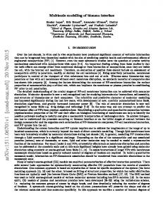
Figure 5 shows an example of an embedded regional ocean model in the northwest Atlantic using the CESM multi-scale ocean configuration. The global ocean is POP at 1 o; the regional model is ROMS at 7 km resolution. The ocean models are two-way coupled. A merged ocean SST is passed to the global atmosphere at each coupling time step, typically at a daily frequency (R. Dussin, pers. comm.). Though conspicuous features such as the Gulf Stream separation are not as skillful as in the pure ROMS hindcast of Kang and Curchitser (2013, 2015), there is an improvement over the coarse resolution global model. This configuration is now being used to explore the effects of the Gulf Stream position and correction of some of the global model biases on downstream climate. Similar models in other boundary currents (e.g., Small et al. 2015) can be used to improve the representation of specific features in a climate model. In spite of increasing computational resources, practical implementation of global highresolution models will remain challenging for some time. This is especially true with Earth System Models that incorporate biogeochemistry. A careful implementation of a nesting strategy is useful to begin exploring the role of the coastal ocean in the climate system and the potential linkages between disparate scales of motion. The technique relies on careful and accurate remapping, which permits conservative interpolation of fluxes. Significant challenges remain in designing nesting strategies for model components other than momentum.

Radiation conditions may not be

appropriate for propagating signals arising from the dominant dynamics in sea ice and biogeochemistry. A final point to be noted is that although high-resolution nests may more accurately represent certain dynamics, such as boundary currents, in and of themselves they cannot correct significant biases that the parent model may contain.

30

Figure 5: NCAR-CESM multi-scale configuration in the northwest Atlantic. The global ocean is POP at 1°; the regional model is ROMS at 7 km resolution. The ocean models are two-way coupled. A merged ocean SST is passed to the global atmosphere at each coupling time step (R. Dussin, pers. comm.).

4. Multi-scale modelling on unstructured grids Unstructured meshes are inherently suited to resolve dynamics encompassing a range of scales. By allowing the size of mesh elements to vary, they offer geometric flexibility w hich goes beyond the functionality allowed by nesting or generalized curvilinear meshes, the two techniques applied commonly to refine on structured meshes. We consider only horizontally unstructured meshes, because the dominance of hydrostatic balance in the ocean demands vertical alignment. Compared to structured meshes, unstructured meshes enable smooth coastlines. Their horizontal density can be adjusted in places where the topographic slope is large, allowing finer topographic

31

details to be better resolved. Many coastal models, designed to use unstructured meshes, benefit from the ability to scale the size of mesh elements with the square root of depth, which allows them to avoid the time step limitation with respect to the speed of surface gravity waves over the deep part of the ocean. Triangular meshes are most flexible and serve as a basis of most models (e.g., ADCIRC (Westerink et al. 1992), FVCOM (Chen et al. 2003), SELFE (Zhang and Baptista 2008), SUNTANS (Fringer et al. 2006) and FESOM (Wang et al. 2014)). Figure 6 (left) shows a patch of such a mesh. Most commonly, the variables are located on mesh vertices, centroids of mesh elements (triangles), or mesh edges. However, higher -order representations are also possible when additional degrees of freedom are introduced inside triangles. Meshes dual to triangular, i.e., obtained by connecting circumcenters of triangles, can also be used, as is schematically shown in the left panel, leading to an arrangement shown in the right panel (see Ringler et al. 2013). We will refer to these as quasi-hexagonal, for hexagons will be met most frequently in this case. The circumcenters should lie inside their triangles, which excludes obtuse triangles. Meshes satisfying this property are called orthogonal. The dual mesh in this case presents the Voronoi tessellation. In principle, there is no limitation on the polygon type, and generalized meshes combining different polygons, for example triangles and quads, are also possible. The question is rather their numerical stability, for mesh heterogeneity may contribute to locally increased errors. Below we will use triangular meshes as an example. a. Examples of unstructured grid techniques To illustrate the basic approaches for horizontally unstructured meshes we consider the 2D advection-diffusion equation for a tracer T,  tT    (uT  K T )  0

32

(1)

with  = (∂x, ∂y) and insulating lateral boundary conditions. Here u is the horizontal velocity vector, and K the diffusivity. For simplicity, we will also consider the 1D version of this equation

 tT   x (uT  K  xT )  0

when describing discretizations. b. Finite volume methods There are several possible ways to discretize the equations of motion on unstructured meshes. The first one relies on reformulating equations so that they express balances related to control volumes, hence the name finite volume (FV) method. In the simplest case when variables are located at the centers of triangles, the control volumes (also referred to as cells) are the mesh triangles proper. If they are at vertices, the so-called median-dual control volumes are routinely used. They are formed by connecting centroids to the centers of edges. The other option is to connect the circumcenters, but this is only possible if the circumcenters are inside their respective triangles. On a regular patch shown in Figure 6 these options coincide, but they differ on general meshes. The FV method relies on the fact that the motion equations have the form of conservation laws, as Eq. (1) above. These equations are integrated over control volumes and their flux divergence term is expressed, via the Gauss theorem, in terms of fluxes out of the control volumes. Due to this strategy, local and global balances are ensured on the discretized level. We apply the FV method to Eq. (1) with cell-centered placement of variables. Indices c, v and e will be used to designate the cells, vertices and edges, respectively. Integrating over a triangle c one obtains

33

 t  Td c   Fe  nele  0.

(2)

e(c)

Here e(c) is the symbolic notation for the indices of the edges of triangle c, ne is the outer normal to the edges, and le their length. The discrete tracer values are introduced as Tc = ∫TdΩc/Ac, where Ac is the triangle area. Note that no approximation is involved in deriving (2). The essence of the FV approach lies in estimating fluxes in terms of cell-averaged values Tc. The language of fluxes automatically ensures that total tracer is conserved. Assuming the velocity field to be given, fluxes can be estimated if the field T is known at the boundary of the control volume.

Figure 6. A regular patch of triangular mesh (left) and hexagonal mesh (right). Such meshes are dual to each other. In triangular case, the degrees of freedom are most frequently located at vertices, centroids or circumcenters, or in the case of C-grid discretization, at mid-edges. For the hexagonal mesh, it is commonly centers of cells or mid-edges in the case of C-grid discretization. This can be done by designing a polynomial reconstruction valid in the cell and its vicinity Tc(x)=a0+a1x+a2y+..., where x and y are coordinates measured from the centroid, and ai the expansion coefficients, such that it satisfies the strong constraint ∫TcdΩc = TcAc and weak constraints minimizing L = Σn(c) (∫TndΩn – TnAn)2. Here n(c) is the list of the neighboring triangles. The number of neighbors involved in the reconstruction depends on its order. Only the nearest 34

neighbors (3 triangles sharing edges with c) are needed for linear least-squares reconstruction, and generalizations of this scheme are straightforward. The higher the order of the reconstruction the more accurate is the estimate of fluxes leaving/entering the control volume. However, for each edge the estimates coming from triangles sharing it are generally different. The flux entering Eq. (2) is therefore some combination of, for example, centered or upwind-biased estimates. On uniform meshes, the first choice will leave a dispersive error, while the second one will lead to a diffusive error. This behavior will be preserved if meshes vary smoothly. One can also reconstruct gradients of T on centered and upstream-biased stencils and use them to estimate T at edges, or combine field reconstruction on several stencils to obtain a weighted essentially non-oscillatory (WENO) scheme. The details here depend on the variable placement. For example, for vertex placement of variables the language of gradient reconstruction turns out to be more convenient because gradients are easily estimated on triangles. Obtaining a monotonic scheme requires limiters or flux-corrected transport algorithms. Since directional splitting is not possible in the horizontal plane, these algorithms prove to be more computationally expensive than their structured-grid counterparts. Note lastly that reconstruction of velocity fields on unstructured grids must be carried out carefully to avoid unintended inaccuracies (see, e.g., Wang et al. (2011)). c. Finite element methods The finite element (FE) method relies on expanding the ocean fields in a series of polynomial basis functions defined on mesh elements, and seeking the coefficients of these expansions from the requirement that the governing equations be satisfied in an optimal way. We introduce a set of basis functions Nj(x,y) defined on mesh elements (in the FE method this name is routinely used instead of volumes or cells in the case of FV) and expand the tracer 35

field as T=Tj(t)Nj(x,y), with summation implied over the repeating indices in this section. The coefficients of expansion are only a function of time, which will be implied below. Depending on the choice of functions the index j can list mesh elements (triangles) or their vertices, edges or additional nodes in elements. A simple example is the continuous P1 representation (P stands for polynomial, and 1 for its degree) in which case Nj(x,y) equals 1 at vertex j and goes linearly to zero at neighboring vertices. In this case T=Tj(t)Nj(x,y) represents a linear interpolation which is continuous across the faces. Continuous quadratic P2 representation deals with functions defined at vertices and mid-edges. Many other possibilities are described in traditional courses on the FE method such as Zienkiewicz and Taylor (2000). It is important to stress that, despite the nonuniform placement of the degrees of freedom Tj, the field T becomes defined over the entire mesh. Since this representation is based on a finite set of degrees of freedom, it cannot satisfy the continuous motion equations exactly. Instead, one requires Eq. (1) be satisfied in a weak sense as

 (M  T  F M )d   0 i t

h

i

(3)

where Mi is an appropriate test function, and integration by parts has been performed to reduce the order of derivatives applied to T. No difficulties occur in this case if the representation for T is continuous, which will be assumed. Clearly, the set of Mi should be sufficient to constrain all the degrees of freedom used to represent T. An obvious possibility is to take Mi=Ni to obtain M ij  tT j  ( Aij  Dij )T j  Si

(4)

where Mij = ∫NiNjdΩ, Aij = -∫Nju · NidΩ and Dij = ∫Kh (Ni)(Nj)dΩ are respectively, mass, advection and diffusion matrices. Note that derivatives in expressions for matrices Aij and Dij would be singular if Nj were discontinuous. The approach implemented in (4) is known as continuous Galerkin (CG) discretization. It is optimal in the sense that the residual of the equation 36

for the field T in the space of basis functions Nj is orthogonal to these functions. A reader should notice that the procedure relies on a scalar product introduced over the space of functions Nj. This proves helpful, for it offers a natural representation for the balance of tracer variance or energy in the case of the primitive equations. Note that in contrast to finite-difference or FV treatments, the time derivatives are coupled through the mass matrix (Mij above). It is non-diagonal for the CG discretization and links all degrees of freedom. The presence of mass matrices improves accuracy, as we shall see below, by reducing numerical dispersion (see, e. g., for more detail Donea and Huerta (2003)), but iterative solvers must then be used to disentangle ∂tTj. Diagonal, or lumped, approximations are sometimes selected for Mij to reduce computational burden, but this has an adverse effect on accuracy. Discontinuous finite elements can be considered a generalization of both FV and CG FE approaches. In this case, the polynomial representation for T is confined to element interiors, and is discontinuous across the elemental boundaries. The simplest example is P0, wherein T is elementwise-constant. For the P1 discontinuous representation, the vertex values are different on each element, so that if six triangles meet at vertex v, there will be six values of Tv there. This leads to clustering of degrees of freedom, so that other variants with internal placement should be preferred. Because of the discontinuous representation, one writes the weak formulation by integrating over element interiors,

 ( (M  T  F M )d    M Fnd  )  P  0 i t

h

i

c

c

(5)

c

where the integration in the last term is over the boundary of element c. Since elements are disconnected, (5) is incomplete unless certain penalties are added, represented here through P. 37

They include terms which weakly impose the continuity of fluxes and fields. An alternative approach is to consider fluxes F as ‘numerical’ fluxes, combining flux estimates from elements across the face together with relevant continuity constraints needed for accuracy and stability. If Mi=Ni, the result is the discontinuous Galerkin (DG) discretization. The reader is advised to consult a regular course (e.g., Li 2006) for details which are numerous here. Compared to the FV method, the DG FE method spares the need for high-order reconstructions if high-order representation is used. This representation is internal to the element, which is beneficial from the standpoint of parallelization. Likewise, mass matrices now connect only local degrees of freedom inside elements, which makes their direct inversion feasible, in contrast to CG FE. This makes the DG FE method appealing for ocean modelling. However, the computational burden is high, and practical applications are still rare (see, e.g. Dawson et al. 2006; Kärnä et al. 2012). Besides, the complexity of coastlines and bottom topography is the reason why geometrical refinement and low-order discretizations are preferred. d. Elementary examples In order to explain how FV and CG FE methods work (we skip the DG FE case as it requires more lengthy detail) we consider a 1D example assuming the velocity u to be uniform. For the FV method, let Tc be the cell-mean value in cell c. The cell length will be hc, and its boundaries will be at xc-1/2 and xc+1/2 = xc-1/2+hc, with the index c increasing in the positive x-direction. We get Tc  ( Fc 1/2  Fc 1/2 ) / hc  0.

For advection, a local linear reconstruction Tc+1/2 = (Tc+1hc+Tchc+1)/(hc+hc+1) will lead to a scheme that is equivalent to standard centered differences on uniform meshes. Note that for linear reconstruction the difference between the cell-mean and cell-centered values can be ignored, but 38

is essential in higher-order reconstructions. If u>0, the estimate for the advective part of the flux Fc+1/2 =uTc will yield the first-order upwind method, and the upwind quadratic reconstruction based on Tc-1, Tc and Tc+1 will lead to a second-order method on a uniform mesh. In order to increase the accuracy of discretization, instead of accurate representation of fluxes one has to concentrate on representing the flux divergence, and follow the road discussed, for example, by Webb et al. (1998). No further detail will be provided here for the reconstructions are specific to the mesh geometry. The important statement, however, is that on general triangular or hexagonal meshes similar procedures are possible as on regular meshes and that will yield discretizations familiar from finite differences in many cases. The computational effort will be higher however, for one cannot rely on a regular stencil. As concerns the diffusive part of the fluxes, one estimates (∂xT)c+1/2 = 2(Tc+1-Tc)/(hc+1+hc) in the 1D case. More generally, the centered combination of diffusive fluxes computed on neighboring control volumes is used. To illustrate the case of CG FE, we place the degrees of freedom Tv at ‘vertices’ located at xv, with the index increasing in the x-positive direction. The P1 basis function associated to vertex v is Nv=1-(x-xv)/hv+1/2 for xv≤x≤xv+1 and Nv=1+(x-xv)/hv-1/2 for xv-1≤ x≤xv and zero otherwise. Here hv+1/2=xv+1-xv and hv+1/2=xv-xv-1. Performing computations of the entries of the matrices, we get

M vj  tT j 

hv 1/2 h  t (2Tv  Tv 1 )  v 1/2  t (2Tv  Tv 1 ), 6 6 AvjT j  (u / 2)(Tv 1  Tv 1 ),

and

DvjT j 

K hv 1/2

(Tv  Tv 1 ) 

39

K hv 1/2

(Tv  Tv 1 ) .

Taking for simplicity the case of uniform mesh, hv+1/2 =hv-1/2=h,  t (Tv 1  4Tv  Tv 1 ) / 6  (u / (2h))(Tv 1  Tv 1 )  K (Tv 1  2Tv  Tv 1 ) / h 2  0.

We now easily recognize that the expressions for advection and diffusion are just the traditional centered differences. The novel feature is the presence of the mass matrix with the time derivative. Because of the mass matrix, the time derivative is weighted over the same stencil as the space derivative. To understand why this is important, we turn to the von Neuman analysis discussed above, taking T=T0(t)eikx. In this case, we get (2+cos kh)∂tT0/3+u(sinkh)T_0+K(2-cos(kh))T0=0 meaning that the phase velocity becomes cp=3(u/kh)sin(kh)/(2+cos(kh)) which ensures much more accurate behavior for small kh compared to the estimate cp=(u/kh)sin(kh) which will follow in the absence of the mass matrix and will also be the result for the FV case above. To conclude, on uniform meshes both FV and linear FE lead to expressions recognizable from finite differences. This situation persists in 2D, and one would derive the same statements on regular quadrilateral meshes. The methods are thus generalizations of common technology to rather arbitrary polygonal meshes. They are more expensive, because the information on neighbors has to be retrieved from look-up tables, as well as information on coefficients of differential operators, which have to be computed in advance to minimize run-time effort. e. Numerical considerations in the primitive and shallow water equations While the considerations above focus on explaining the essence of unstructured numerical methods, it leaves aside an important question of the consistency between the representation of velocity and scalars (pressure and tracers). Similar to the difference in numerical properties of solutions on the Arakawa A, B and C grids, the properties of solutions on unstructured meshes also depend on the placement of 40

variables. The collocated placement of velocities and scalars is equivalent to the A grid and shares a similar difficulty, namely the presence of a pressure mode on uniform meshes. A pressure mode is the possibility of non-trivial pressure distribution that corresponds to zero pressure gradient. It occurs because of gradient averaging implied by collocated meshes. Additionally, on such meshes the discrete curl of pressure gradient in the discretized momentum equation is not necessarily zero, which introduces errors in the discrete vorticity balance. Both call for stabilization in geostrophically dominated regimes, which introduces errors in the energy balance. Although collocated placement of variables is popular in computational fluid mechanics because the same infrastructure is shared by all variables, there is a tendency toward the use of codes with staggered placement of variables, which are free of pressure modes if there is no gradient averaging, in ocean modelling. Staggered triangular grids, however, encounter a geometrical difficulty. The ratio of the number of vertices to cells to edges is 1:2:3, so that, as a rule, a staggered discretization will not be balanced: the number of degrees of freedom in velocity and pressure taken at different locations will be inconsistent, i.e., will deviate from the ratio 2:1. Thus, for example, a cell-vertex (velocitypressure) FV discretization, which is an analog to the B-grid, is characterized by a too large velocity space. A triangular C-grid discretization with normal velocities at edges has too many pressure degrees of freedom. The consequence of the lack of balance is the presence of numerical modes. A review by Danilov (2013) presents a more detailed analysis and contains references to numerous works that have explored the properties of particular discretizations. In summary, there is no perfect staggered discretization, but in some cases the numerical modes can be handled relatively easily. Numerical modes involving extra velocities can be controlled by viscosity; however there is no obvious means to control too large a pressure space. 41

In this respect, the triangular C-grid is a sub-optimal choice, and the preference should be given to its dual implementation, the hexagonal C-grid which has too many velocities. A general issue for C-grid codes is the accuracy of horizontal velocity reconstruction. Codes based on triangular Cgrids are prone to noise in the vertical velocity field in regimes characteristic of the large-scale ocean. They are, nevertheless, popular in coastal or estuarine-scale applications where the noise presents a lesser problem. A quasi-hexagonal C-grid forms the basis of the MPAS approach (Ringler et al. 2013), while the FV cell-vertex discretization is used in FVCOM and in the FV approach of Danilov (2012). Triangular C-grids are the choice of UnTRIM and SUNTANS. FESOM (Wang et al. 2014) is an A-grid model relying on CG FE, as does ADCIRC. Although initial development of unstructured-mesh ocean models was distributed between the CG FE and FV methods, current understanding is in favor of the FV method. The reason is that the hydrostatic approximation used by models and the need to have a clear definition of fluxes both encounter difficulties in the CG FE implementation. The horizontal coupling of CG FE makes the hydrostatic balance horizontally non-local, while breaking this coupling destroys energetic consistency. Although CG FE codes can be made perfectly volume conserving, they treat conservation in the weighted sense, without resorting to fluxes. The interest in DG FE and in spectral element methods persists, yet at present they are associated with an overly large computational burden. f. Meshes, resolution and practical examples The practical recipes on how the mesh resolution should be varied depend on the application and differ on regional and large scales. On regional scales, if the dynamics are tidally driven, scaling the mesh element size as (gH)1/2, with g the acceleration due to gravity and H the

42

fluid thickness, could be advantageous since such meshes are ‘uniform’ in terms of the propagation speed of surface gravity waves. Making cells on the deep water larger helps to circumvent time step limitations that will occur otherwise. Extra resolution may, however, be needed to resolve steep or sharply varying topography, or to resolve estuaries or details of coastlines. Many examples of successful applications demonstrating the utility of this approach can be found, for example, on the web sites of such models as FVCOM or ADCIRC, and the review by Greenberg et al. (2007) discusses many associated aspects. Such highly variable meshes are not necessarily optimal in other situations involving baroclinic dynamics, instabilities and eddies. Here the point is that numerical and physical dissipation depends on resolution and smaller dissipative coefficients are used on finer meshes. The implication is that a mesh optimal for simulating tides can be sub-optimal for simulating baroclinic dynamics because of enhanced dissipation across its coarse mesh. Such applications would benefit from certain mesh uniformity, and the unstructured mesh character has only to provide a mechanism for effective nesting. The mesh design is then very similar to that sought by nested structured-grid models, with the difference that technical nesting can be avoided. This situation is also common for large-scale applications. In this case, there are two main factors motivating the use of unstructured meshes. The first is once again the effective nesting motivated by the need to resolve eddies, as demonstrated by Ringler et al. (2013). The other factor is the geometry of important straits, as in the study by Wekerle et al. (2013). In all cases it shoul d be borne in mind that dissipation, especially spurious numerical dissipation, is linked to resolution, and by refining, one takes into account smaller flow details and simultaneously activates a part of dynamics that was previously damped on resolved scales. From the consideration of numerical stability and accuracy smooth mesh transitions should be preferred, for this minimizes residual 43

errors in representation of discrete operators. There are physical consequences too, for baroclinic instabilities and eddies do not saturate immediately, and the presence of a coarse or eddypermitting mesh upstream may affect the dynamics downstream in the refined domain. Study of all numerical aspects associated with variable resolution is only beginning. Questions on how to deploy resolution are closely related to time integration. In the nested mode, the time step of an unstructured-mesh code will be defined by the size of the smallest element. Such codes will then be numerically efficient only if the smallest elements use an overwhelming number of degrees of freedom. This is easy to achieve in some situations, and this may be the reason of reduced numerical efficiency in some others. Generally this implies the need for careful consideration of many related issues and much experimentation with alternative approaches. 5. Parameterizing unresolved and partially-resolved phenomena In ocean modelling, an approximation of the effects of unresolved processes in terms of resolved and known quantities is called a parameterization. In other fields, the terms subgrid model, closure, or regularization are used, which reflect that the unresolved processes 1) lie below the resolution of the grid, 2) are required for the equations of motion to be closed, and 3) tend to regularize or eliminate singularities that may arise in their absence. The most important consideration in determining the parameterizations required in an ocean model is determining which processes are resolved, which are not, and which are partially resolved. In unstructured grid models, this determination is even more important. In hierarchies of models of varying resolution or nested grid modelling, these determinations can help to ensure that equivalent scenarios are being simulated among the models.

44

Parameterizations may be crude or sophisticated, and they are rarely insignificant to the outcome of the simulation. If they were they would be neglected, for reasons explained below. Standard fluid viscosity and diffusivity themselves are parameterizations: they approximate the average over many stochastic trajectories of molecules under the assumptions of local equilibrium and typically also isotropy or transverse isotropy (e.g., when vertical and horizontal directions are distinguished). On scales near the mean free path of molecules, these approximations break down. In situations featuring strongly non-equilibrium thermodynamics, thermal diffusivity fails. NonNewtonian fluids are still treatable as viscous fluids, but with generally non-linear constitutive relations between stress and rate of strain, rather than a simple proportionality with a viscous coefficient between stress and rate of strain. In fluid modelling, turbulence is the most common feature requiring parameterization. The idea of an eddy viscosity or eddy diffusivity - a value much larger than the molecular one to treat turbulent eddies similarly to molecular motions – predates computational modelling (e.g., Boussinesq 1877; Ekman 1905). However, turbulence is not necessarily confined to a largest scale that plays the role of the mean free path, and therefore a scale separation between resolved features and unresolved turbulence may not be realized. Furthermore, geophysical turbulence is frequently anisotropic and heterogeneous, and parameterizations may reflect this broken symmetry to greater or lesser degree. A lack of scale separation complicates the development and generality of parameterizations significantly. When there is a scale separation between the largest turbulent features and the grid scale, the equations can be cast in terms of predicting only the Reynolds average of the motion, which may be steady, slowly varying, and/or easily resolved. Simulations without scale separation can be termed Large Eddy Simulations (LES), as only the largest of the turbulent features are

45

resolved and smaller ones are parameterized. In Reynolds-averaged parameterizations, the modest changes in resolution of the model may not affect the parameterization. In LES, the eddy viscosity typically depends on the resolution of the model and also the flow. Likely the most common eddy viscosity parameterization is that of Smagorinsky (1963) based on the energy cascade idea of Kolmogorov (1941), which has precisely these characteristics:  x  S      

2

1  ui uk  ui uk      , 4  xk xi  xk xi 

where Einstein summation is implied on indices, and the dimensionless constant Ƴ is near 1. The Smagorinsky viscosity depends on both the velocity u and gridscale Δx. Because of these scalings, the rate at which energy is dissipated can be matched to the rate at which it is flowing from large to small scales in the resolved flow, which mimics the effects of a longer turbulence cascade (i.e., higher resolution). Although the Smagorinsky viscosity is in wide use in nonhydrostatic simulations, it is not appropriate for use in the large-scale enstrophy cascades of rotating fluids later discovered by Kraichnan (1967) as an integral critical in the derivation of the viscosity diverges in an enstrophy cascade (Fox-Kemper & Menemenlis 2008). The three-dimensional form above is the correct one for use in nonhydrostatic models where all velocity components are treated similarly. Smagorinsky (1993) also derives a hydrostatic version which only involves the horizontal velocities, and forms for anisotropic grids require more care (e.g., Ramachandran et al. 2013). For a derivation of the Smagorinsky closure for hydrostatic and nonhydrostatic models, see Smagorinsky (1993) or Fox-Kemper and Menemenlis (2008). Even though Smagorinsky developed this parameterization for use in atmospheric models, it is not suitable for most simulations of large-scale atmospheric and oceanic flows which 46

commonly use hydrostatic approximations and anisotropic grids. At large scales, the effects of rotation (quantified by Rossby number Ro = U/fL), stratification (quantified by Richardson number Ri = N2/(∂U=∂z)2), and the limited aspect ratio (α = H/L) of motions wider than the depth of the ocean all prevent the occurrence of isotropic three-dimensional (3d) turbulence. In stratified fluids, only scales smaller than the Ozmidov scale (the square root of energy flux divided by N 3) or the Thorpe scale are observed to have turbulence resembling a 3d cascade. Dillon (1982) shows that these scales are frequently related and O(1m) in the upper ocean at a variety of sites— obviously, these scales are much smaller than the grid scale used in large-scale ocean and atmosphere modelling. Perhaps these scales might be resolved by the vertical grid, but not the horizontal: is an anisotropic form of Smagorinsky appropriate in that case?

Even anisotropic

forms of the Smagorinsky scheme continue to be derived from Kolmogorov theory for 3d turbulence with a forward energy cascade (e.g., Ramachandran et al. 2013). In large-scale oceanic turbulence, the forward energy cascade is not usually in effect until very small scales, and a cascade of enstrophy or potential enstrophy may be more relevant on the scale of the model grid. Then, the Leith (1996) scheme or adaptations of it (Fox-Kemper and Menemenlis 2008; Bachman et al. 2017; Pearson et al. 2017) are preferable. One day, large-scale ocean simulations will reach the point where the grid scale is firmly within the range of scales where Kolmogorov turbulence is expected, as presently occurs in boundary layer LES (Sullivan and Patton 2011), but at present rates of increasing computational power, this day is centuries away for global simulations and decades away for most coastal applications. In the meantime, it is important to distinguish between partially-resolved processes— requiring parameterizations to be scale-aware, or scale with resolution--and processes that are firmly below the grid scale—for which parameterizations may be less dependent on grid scale. In

47

typical ocean models, mesoscale and submesoscale eddies are partially resolved, justifying a scaleaware LES approach to handling these phenomena (e.g., Pearson et al. 2017). However, boundary layer and breaking internal wave turbulence, which are expected to cascade into the 3d turbulence, but only with O(1m) grids and nonhydrostatic models, are far from being resolved. Thus, these processes are likely to be approximated with Reynolds averages and parameterizations that do not depend on modest changes to the scale of the grid, such as a background eddy diffusivity. Sometimes, even Reynolds average schemes are flow-aware (i.e., they depend on resolved flows in a nontrivial way) and therefore must also become scale-aware to account for the dependence of the resolved flow resolution. For example, the submesoscale restratification parameterization of Fox-Kemper et al. (2011) incorporates the strength of resolved density gradients to infer the strength of unresolved fronts. At coarse resolution, the resolved density gradients are sensitive to changes in resolution, so the parameterization depends on the grid scale to approximately account for this lack of convergence. In this Reynolds-averaged but flow-aware case, the goal is to keep the effect of the unresolved phenomena unaffected by changes in the grid scale. By contrast, LES schemes are scale-aware to make parameterizations of partially-resolved phenomena be affected by grid scale, so that the parameterization effect is reduced as the grid is refined. Therefore, parameterizations must not only account for the effects of unresolved motions, but be sensitive, or scale-aware, as to what kinds of motion are or are not resolved. For example, the majority of present atmosphere and ocean models are hydrostatic, which is a good approximation when the aspect ratio of the resolved motion is small. However, hydrostatic motions cannot exhibit a Kolmogorov 3d cascade, which requires an equality among velocities in all directions. Thus, when the grid aspect ratio is small and the model is hydrostatic, it is not consistent to use a Kolmogorov-based LES parameterization, such as the Smagorinsky scheme, because then

48

the physical parameterization assumes no scale separation from 3d turbulence while the numerics demands a scale separation. However, the Smagorinsky scheme is frequently used outside of its realm of theoretical applicability, because it is numerically robust, scale-aware, and flow-aware despite being inaccurate in such applications (Griffies and Hallberg 2000). In such models, the effects of 3d turbulence should be included through Reynolds-averaged boundary layer schemes, and other scale-aware and flow-aware schemes should be used that are suited for the partiallyresolved phenomena. Dimensional analysis based on the grid scales, coupled with dominant balances expected by the flow regime, can reveal important aspects of the motion near the grid scale useful in developing or choosing among parameterizations (e.g., Bachman et al. 2017). On much larger scales, when the Rossby number is small and the Richardson number is large, then the horizontal scale of motion may be larger than the deformation radius (quantified by the Burger number Bu = (Ld/L)2 ≈ Ro2Ri). When a model grid has a small or O(1) Burger number, then the turbulence near the gridscale is quasi-geostrophic (QG), and a different set of turbulence cascades may be used to construct LES parameterizations. At the same time, the effects of 3d turbulence, for example in boundary layer schemes, may also be included with an assumed scale separation. Likewise, on very large scales, then barotropic motions may be approximated as 2d turbulence. Fox-Kemper and Menemenlis (2008) give examples of closures suitable in these regimes, while other closures rely on spectral self-similarity but do not specify what kind of selfsimilarity to expect (e.g., Bardina et al. 1980; San et al. 2011, 2013). Examples of processes for which parameterizations that presently exist are: mesoscale (Gent and McWilliams 1990; Redi 1982; Treguier et al. 1997; Griffies 1998; Eden and Greatbatch 2008; Jansen and Held 2014; Bachman and Fox-Kemper 2015; Grooms 2016; Bachman et al. 2017; Pearson et al. 2017; Zanna et al. 2017), submesoscale (Fox-Kemper et al. 2008; Fox-Kemper

49

et al. 2011), boundary layer turbulence (Kraus and Turner 1967; Mellor and Yamada 1982; Price et al. 1986; Large et al. 1994; Sullivan et al. 1994; Canuto et al. 2001; Harcourt 2013; Li et al. 2016), tidal mixing (Jayne and St Laurent 2001), fine-scale mixing by internal gravity waves (Polzin et al. 2014), symmetric instabilities (Bachman et al. 2017a), surface gravity waves (Longuet-Higgins and Stewart 1962; Craik and Leibovich 1976; Lane et al. 2007), air-sea fluxes (Large and Pond 1981, 1982; Edson et al. 2013), bubbles (Liang et al. 2011), sediment (Warner et al. 2008), estuaries (Garvine and Whitney 2006; Sun et al. 2017), albedo (Payne 1972; Brandt et al. 2005), ice-ocean fluxes (McPhee et al. 2008), convection (Killworth 1989; Ilcak et al. 2014), abyssal overflows (Yeager and Danabasoglu 2012), skin layers and diurnal layers (Large and Caron 2015), biophysics (Zhang et al. 2009), and many more processes. Process studies - using high-resolution models or observations - of each phenomenon, spanning a hopefully representative set of scenarios, are generally the key to parameterization development and evaluation. The reader may note that the majority of phenomena requiring closures just mentioned are turbulent or at least nonlinear. This results from the need to parameterize only those motions that can communicate across scales from unresolved to resolved. Scale connectivity is a defining aspect of turbulence, and all nonlinear phenomena have the potential for scale connectivity. Dominantly linear phenomena, such as waves in the absence of mean flow, stratification, or topography variations, do not link strongly across scales, so unresolved waves of this type do not interact with resolved flows. One important exception occurs at surface and bottom boundary layers, where many phenomena require parameterization to appropriately accept stress and energy forcing (generally using a Reynolds average approach). Mathematically, neglecting these effects produces singular perturbations of the equations of motion thereby eliminating whole categories of possible solutions.

50

An advantage of scale-aware parameterizations is that they tend to regularize singularities regardless of grid scale and therefore result in robust numerical stability. The Boussinesq, hydrostatic primitive equations common to ocean and atmospheric simulations are well-behaved mathematically, but some mechanisms of regularization are required for this to be true ( Cao and Titi 2007; Cao et al. 2013). Even in structured grid modelling, variation in latitude or stratification can change the effective scale of phenomena, and make constant viscosities and diffusivities fail to regularize the flow sufficiently for a given grid scale. In unstructured and variable grid modelling, such considerations are paramount for accurate and stable simulations. However, physical parameterizations are often more complicated, e.g., strongly nonlinear or flow -dependent, which may mean that while they tend to regularize, it may be impossible to prove that fact. Examples of stability and improved simulation fidelity through physical parameterizations include Griffies and Hallberg (2000), Fox-Kemper and Menemenlis (2008), Chen et al. (2011) and Ilicak et al. (2012). There are some disadvantages of physical parameterizations to keep in mind as well. The most obvious is that they may make the simulation more costly (parameterizations cost typically 10 to 25% of the total), and therefore reduce the achievable model resolution which is almost always desired. So, parameterizations should be judged based on impact versus cost, and designed with attention to balancing increased accuracy versus increased complexity. Additionally, the generally-idealized process studies used to develop a parameterization are typically not representative of all scenarios that may be encountered in realistic modelling. It is common for a parameterization developed in extra-tropical process studies to fail in applications near the equator. In addition, parameterizations introduce imperfectly-known constants or parameters and thus additional uncertainty into models. Clever approaches to exploit these uncertainties rely on tuning

51

the parameter values to reduce model to observation mismatch, or better yet to produce ensembles of simulations of varying parameter values to map and quantify the consequences of uncertainties. Tuning is a dangerous business, because often the right answer can be arrived at for the wrong reasons, which may significantly affect model sensitivity or behavior in unprecedented forcing regimes (such as climate change). A good example of this effect is that often when a new parameterization, with solidly-grounded physics based on process modelling or observations, is introduced into a model previously lacking a representation of said physics, it often increases the biases and mismatches in the model solutions versus observations. This is not an indication that the model has been degraded in realism, but that it was previously tuned to mask the neglect of a phenomenon with a canceling error in the values of other parameters chosen. Once the new phenomenon receives treatment, the erroneous values of the other parameters resulting from tuning are exposed and require readjustment. Finally, the nonlinear character of most parameterizations may preclude or limit their use in certain circumstances, as do some types of data assimilation that do not require adjoints (e.g., ensemble Kalman methods). Finally, it is easy to oversimplify parameterizations, e.g., substituting a horizontal diffusivity for an along-isopycnal diffusivity or an isotropic scalar diffusivity where an anisotropic tensor diffusivity is more appropriate, and it may be difficult to identify the consequences of these oversimplifications without careful thought and comparison to observations (Veronis 1977; Fox-Kemper et al. 2013). Some numerical schemes seek to regularize, or otherwise constrain solution characteristics, without attempting to reproduce a particular physical phenomenon. Common examples are upwinding, monotonic, and shock-capturing schemes. Generally, these methods arrive at the cost of low-order accuracy, but low-order accuracy is typical in unstructured grid modelling in any

52

case. A closely related idea is that of mimetic schemes, which seek exact mimicry of conservation laws in the continuous equations (for energy, enstrophy, potential density, mass, etc.) in the discrete equations. These schemes inherently offer regularization benefits. For example, if energy is conserved, it is impossible for an instability to cause unbounded growth in energy. However, these schemes are often slower to converge and less formally accurate than non-conservative schemes, e.g., spectral methods. It is easy to prove the effectiveness of such schemes, because conservation is guaranteed. However, it is difficult to prove that choice to be optimal, because other aspects of the solution are degraded in exchange. Furthermore, mimetic and constrained schemes are not a replacement for accurate physical parameterizations. For example, there are many pathways where energy is transferred among scales, and so exact conservation of resolved energy would be incorrect. Consider the example of boundary layers in oceanic and atmospheric flows. These layers have significantly more turbulent energy from surface roughness, waves, and convection—all of which is injected on scales smaller than a typical large-scale model grid, yet these energetic regions tend to perform important mixing of the larger scale property gradients. Conserving energy on the large scale grid is no substitute for these unresolved phenomena in terms of ocean model accuracy, unlike in engineering LES or DNS applications where small -scale energy is dwarfed by larger scale flows. Thus, scale-aware physical parameterizations may be used together with mimetic schemes to arrive at realistic flows of energy, enstrophy, or other desired quantities. Examples of accuracy and improved simulation fidelity through such schemes are Lax and Wendroff (2005), Leonard (1979), Zalesak (1979), Friedrich (1998), Nadiga and Bouchet (2011) and San et al. (2011, 2013). Most modelling approaches blend together the physical aspects of parameterizations of unresolved processes with numerical accuracy, convergence, and regularization concerns, such as

53

grid scale, altered vertical coordinate discretization, including Lagrangian or semi-Lagrangian approaches. As such the desired overall effect may be realized, but care is needed, e.g., in adapting a parameterization that is successful in a pressure coordinate model into a model using isopycnal coordinates. A general approach to these issues is not yet known, but these steps become an active topic of research each time a new modelling system is developed.

6. Final remarks: numerical modeling in a multi-component ocean Ocean prediction systems require several integrated components. A central element in these systems, discussed here, is a time-evolving numerical circulation model based upon the oceanic equations of motion (Jacobs and Fox-Kemper 2017). Equally important however are, first, in situ and external data collection systems necessary to provide the information required for initial and boundary conditions, and second, data assimilation methodologies to impose internal datadriven constraints. These issues are reviewed in this volume by, among others, Brink and Kirincich (2017) and Lermusiaux (2017a,b). One over-riding constraint on our ability to deliver improved, high-resolution numerical forecasts is the competition between the computational cost of our prediction systems and the rate of increase in computer power (i.e., Moore’s Law). In addition to the continuing delivery of additional raw computer power, consequential improvement has also been consistently achieved through enhancement in the computational algorithms used for numerical solution, data assimilation, etc. The implementation of multi-scale discretization procedures, such as the nested and unstructured grid techniques reviewed here, are examples of the latter means of achieving gains in efficiency.

Alternative numerical approaches are continually under development;

54

additional examples include moving grid methods (Koltakov and Fringer 2012), and higher-order finite element and mortar element methods (Iskandarani et al. 2002; Maday et al. 1989). Lastly, we have focused here primarily on numerical treatments for the multi-scale ocean circulation, i.e., ocean physics.

For the reasons noted here, this has been, and will remain, an

unavoidable concern in Earth System Model design. Of perhaps equal concern, however, is the increasing cost and complexity of including specialized modules for other geomorphological, chemical, ecological and cryospheric processes, i.e., the multi-component ocean. Especially over the long time scales of concern to climate modelling and prediction, the linkages between the ocean circulation and these other processes are all of significant concern. As a consequence, in parallel with the development of multi-scale treatments such as those described above, whole new categories of coupled marine models have been, and are being, developed to address particular concerns. These include integrated models that incorporate the effects of waves and tides, currents and sediment transport (Egbert and Ray 2017; Kirby 2017), geochemical cycling (Hofmann 2008), physical/biological interaction (Curchitser et al. 2013), iceocean coupling (Bartino and Holland 2017), and many other processes. Integrations of multi-component systems of significant duration are now routinely feasible on many space scales - e.g., estuarine (de Brye et al. 2010; Powell et al. 2012), continental shelf and slope (Previdi et al. 2009), basin-scale (Hermann et al. 2009), and global (Miller at al. 2017). Despite continued enhancement in computer capacity, the next step forward -- end-to-end coupled Earth System Models that allow affordable integration over extended time scales on global, multiscale domains – will ensure the continuing need for novel new numerical approaches.

55

Acknowledgements The authors gratefully acknowledge the constructive suggestions of the anonymous referees. BFK was supported by NSF 1350795.

REFERENCES Arakawa, A. 1966. Computational design for long-term numerical integration of the equations of fluid motion: Two-dimensional incompressible flow. Part I. J. Comp. Phys., 1, 119-143. Bachman, S. D., Fox-Kemper, B. and Pearson, B. 2017. A scale-aware subgrid model for quasigeostrophic turbulence. Journal of Geophysical Research-Oceans, 122, 1529-1554. Bachman, S.D., Fox-Kemper, B., Taylor, J. R. and Thomas, L. M. 2017a. Parameterization of frontal symmetric instabilities. I: Theory for resolved fronts. Ocean Modelling, 109, 72-95. Bardina, J., Ferziger, J.H. and Reynolds, W.C. 1980. Improved subgrid-scale models for largeeddy simulation. In: American Institute of Aeronautics and Astronautics, Fluid and Plasma Dynamics Conference, 13th, Snowmass, Colo., July 14-16, 1980, 10 p. Bartino, L. and Holland. M. 2017. Coupled ocean-ice modeling and predictions. In The Sea: The Science of Ocean Prediction, special issue, J. Mar. Res., in press. Beckers J.-M. 1992. Analytical linear numerical stability conditions for an anisotropic threedimensional advection-diffusion equation. SIAM Journal on Numerical Analysis, 29, 701-713. Beckers, J-M. and Deleersnijder, E. 1993. Stability of a FBTCS scheme applied to the propagation of shallow-water inertia-gravity waves on various space grids. J. Comp. Phys., 108, 95-104. Biastoch, A., Böning, C. W. and Lutjeharms, J. R. E. 2008. Agulhas leakage dynamics affects decadal variability in Atlantic overturning circulation. Nature, 456, 489–492. Bleck, R. 2002. An oceanic general circulation model framed in hybrid isopycnic-Cartesian coordinates. Ocean Modelling, 4, 55–88. Boussinesq J. 1877. Essai sur la théorie des eaux courantes, Mémoires Présentés par Divers Savants à l'Académie des Sciences, 23, 1-680. Brandt, R. E., Warren, S. G., Worby, A. P. and Grenfell, T. C. 2005. Surface albedo of the antarctic sea ice zone. Journal of Climate, 18, 3606-3622. Brink, K. H. and Kirincich, A. R. 2017. Some considerations about coastal ocean observing systems. In The Sea: The Science of Ocean Prediction, part 1, special issue, J. Mar. Res. 75, 161188. Canuto, V., Howard, A., Cheng, Y., Dubovikov M., 2001. Ocean turbulence. Part I: One-point closure model-momentum and heat vertical diffusivities. J. Phys. Ocean., 31, 1413-1426. 56

Cao, C., Ibrahim, S., Nakanishi, K., and Titi, E. S. 2013. Finite-time blowup for the inviscid primitive equations of oceanic and atmospheric dynamics. Comm. Math. Phys., 337, 473-482. Cao, C., and Titi, E. S., 2007. Global well-posedness of the three-dimensional viscous primitive equations of large scale ocean and atmosphere dynamics. Annals of Mathematics, 166, 245-267. Chanut, J., Barnier, B., Debreu, L., Large, W., Penduff, T., Molines, J.-M., and Mathiot, P. 2008. Mesoscale eddies in the Labrador Sea and their contribution to convection and re-stratification. J. Phys. Ocean., 38, 1617-1643. Chassignet, E., Hurlburt, H.E., Smedstad, O. M., Halliwell, G., Wallcraft, A. H., Metzger, E. J., Hogan, P. J., Blanton, B. and Srinivasan, A. 2006. Generalized vertical coordinates for eddyresolving global and coastal ocean forecasts. Oceanography, 19, 118-129. Chen, C., Liu, H., and Beardsley, R. C. 2003. An unstructured grid, finite-volume, threedimensional, primitive equations ocean model: Applications to coastal ocean and estuaries. J. Atmos. Ocean. Tech., 20, 159-186. Chen, Q., Gunzburger, and M., Ringler, T. 2011. A scale-invariant formulation of the anticipated potential vorticity method. Mon. Weath. Rev., 139, 2614-2629. Choi, B.-J., Iskandarani, M., Levin, J. and Haidvogel, D. B. 2004. A spectral finite volume method for the shallow water equations. Month. Weath. Rev., 132, 1777-1791. Craik, A. D. D. and Leibovich, S. 1976. Rational model for Langmuir circulations. J. Fluid Mech., 73, 401-426. Curchitser, E.N., Haidvogel, D. B., Hermann, A. J., Dobbins, E., Powell, T. M. and Kaplan, A. 2005. Multi-scale Modelling of the North Pacific Ocean: Assessment of simulated basin-scale variability (1996-2003). J. Geophys. Res., 110, C11021. Curchitser, E.N., J. Small, K. Hedstrom and W. Large, 2011. Up- and down-scaling effects of upwelling in the California Current System. pp. 98-102. In: Foreman, M.G., Yamanaka, Y. (Eds), Report of Working Group 20 on Evaluations of Climate Change Projections, PICES Scientific Report No. 40. Curchitser, E., Batchelder, H. P., Haidvogel, D. B., Fiechter J. and Runge, J. 2013. Advances in physical, biological, and coupled ocean models during the US GLOBEC program. Oceanography, 26, 54-69. Danilov, S. 2012. Two finite-volume unstructured mesh models for large-scale ocean modeling. Ocean Modelling, 47, 14-25. Danilov, S. 2013. Ocean modeling on unstructured meshes. Ocean Modelling, 69,195-210. Dawson, C. N., Westerink, J. J., Feyen, J. C., and Pothina, D. 2006. Continuous, discontinuous and coupled discontinuous-continuous Galerkin finite element methods for the shallow water equations, Intl. J. Num. Meth. Fluids, 52, 63-88. 57

Debreu, L., Vouland, C. and Blayo, E. 2008. AGRIF: Adaptive grid refinement in Fortran. Comput. Geosci., 34, 8–13. de Brye B., de Brauwere, A., Gourgue, O., Kärnä, T., Lambrechts, J., Comblen R. and Deleersnijder, E. 2010. A finite-element, multi-scale model of the Scheldt tributaries, river, estuary and ROFI, Coastal Engineering, 57, 850-863. Dillon, T.M. 1982. Vertical overturns: A comparison of Thorpe and Ozmidov length scales. J. Geophys. Res.: Oceans, 87, 9601-9613. Donea, J. and Huerta, A. 2003. Finite Element Methods for Flow Problems. John Wiley and Sons. Döscher, R., Böning, C. W. and Herrmann, P. 1994. Response of circulation and heat transport in the North Atlantic to changes in thermohaline forcing in northern latitudes: A model study. J. Phys. Oceanogr., 24, 2306–2320. Dukowicz, J. K. 1995. Mesh effects for Rossby waves. J. Comp. Phys., 119, 188-194. Durran, D. R. 1999. Numerical Methods for Wave Equations in Geophysical Fluid Dynamics. Springer-Verlag. Eden, C. and Greatbatch, R. J. 2008. Towards a mesoscale eddy closure. Ocean Modelling, 20, 223-239. Edson, J. B., Jampana, V., Weller, R. A., Bigorre, S. P., Plueddemann, A. J., Fairall, C. W., Miller, S. D., Mahrt, L., Vickers, D., Hersbach, H. 2013. On the exchange of momentum over the open ocean. J. Phys. Ocean., 43, 1589-1610. Egbert, G. D. and Ray, R. D., 2017. Tidal prediction. In The Sea: The Science of Ocean Prediction, part 1, special issue, J. Mar. Res. 75, 189-237. Ekman, V. W. 1905. On the influence of the earth's rotation on ocean currents. Arkiv. Mat. Astron. Fysik., 2, 1-53. Fox-Kemper, B., Bachman, S., Pearson B. and Reckinger, S. 2014. CLIVAR Exchanges, 19, 4245. Fox-Kemper, B., Danabasoglu, G., Ferrari, R., Griffies, S. M., Hallberg, R. W., Holland, M. M., Maltrud, M. E., Peacock, S. and Samuels, B. L. 2011. Parameterization of mixed layer eddies. III: Implementation and impact in global ocean climate simulations. Ocean Modelling, 39, 61-78. Fox-Kemper, B., Ferrari, R. and Hallberg, R. 2008. Parameterization of mixed layer eddies. Part I: Theory and diagnosis. J. Phys. Ocean., 38, 1145-1165. Fox-Kemper, B., Lumpkin, R. and Bryan, F. O. 2013. Lateral transport in the ocean interior. In: Siedler, G., Griffies, S. M., Gould, J., Church, J. A. (Eds.), Ocean Circulation and Climate: A 21st century perspective. Vol. 103 of International Geophysics Series. Academic Press (Elsevier Online), Ch. 8, pp. 185-209 58

Fox-Kemper, B. and Menemenlis, D. 2008. Can large eddy simulation techniques improve mesoscale-rich ocean models? In: Hecht, M., Hasumi, H. (Eds.), Ocean Modelling in an Eddying Regime. Vol. 177. AGU Geophysical Monograph Series, pp. 319-338. Friedrich, O. 1998. Weighted essentially non-oscillatory schemes for the interpolation of mean values on unstructured grids. J. Comp. Phys., 144, 194-212. Fringer, O. B., Gerritsen, M. and Street, R. L. 2006. An unstructured-grid, finite-volume, nonhydrostatic, parallel coastal ocean simulator. Ocean Modelling, 14, 139-173. Garvine, R. W. and Whitney, M. M. 2006. An estuarine box model of freshwater delivery to the coastal ocean for use in climate models. J. Mar. Res., 64, 173-194. Gent, P. R. and McWilliams, J. C. 1990. Isopycnal mixing in ocean circulation models. J. Phys. Ocean., 20, 150-155. Gerdes, R., Biastoch, A. and Redler, R. 2001. Fresh water balance of the Gulf Stream System in a regional model. Clim. Dyn., 18, 17–27. Greenberg, D.A., Dupont, F., Lyard, F.H., Lynch, D.R. and Werner, F.E. 2007. Resolution issues in numerical models of oceanic and coastal circulation. Cont. Shelf Res., 27, 1317-1343. Griffies, S. and Hallberg, R. 2000. Biharmonic friction with a Smagorinsky-like viscosity for use in large-scale eddy-permitting ocean models. Mon. Weath. Rev., 128, 2935-2946. Griffies, S. M. 1998. The Gent-McWilliams skew flux. J. Phys. Ocean., 28, 831-841. Grooms, I. 2016. A Gaussian-product stochastic Gent–McWilliams parameterization. Ocean Modelling, 106, 27-43. Harcourt, R. R. 2013. A second-moment closure model of Langmuir turbulence. J. Phys. Ocean., 43, 673-697. Hermann, A.J., Curchitser, E. N., Dobbins, E. L. and Haidvogel, D. B. 2009. A comparison of remote versus local influence of El Nino on the coastal circulation of the Northeast Pacific. DeepSea Res. II, 56, 2427-2443. Hirt, C. W., Amsden, A. A. and Cook, J. L. 1974. An arbitrary Lagrangian–Eulerian computing method for all flow speeds. J. Comp. Phys., 14, 227-253. Hofmann, E., Druon, J.-N., Fennel, K. Friedrichs, M., Haidvogel, D. B., Lee, C., Mannino, A., McClain, C. Najjar, R., Siewert, J., O’Reilly, J., Pollard, D., Previdi, M., Seitzinger, S., Signorini, S. and Wilkin, J. 2008. Eastern U.S. continental shelf carbon budget: Integrating models, data assimilation, and analysis. Oceanography, 21, 86-104. Hofmann, E., Bushek, D., Ford, S., Guo, X., Haidvogel, D. B., Hedgecock, D., Klinck, J., Milbury, C., Narvaez, D., Powell, E., Wang. Y., Wang, Z., Wilkin, J. and Zhang, L. 2009. Understanding

59

how disease and environment combine to structure resistance in estuarine bivalve populations. Oceanography, 22, 212-231. Ilicak, M., Adcroft, A. J., Griffies, S. M. and Hallberg, R. W. 2012. Spurious dianeutral mixing and the role of momentum closure. Ocean Modelling, 45, 37-58. Ilicak, M., Adcroft, A. J. and Legg, S. 2014. A framework for parameterization of heterogeneous ocean convection. Ocean Modelling, 82, 1-14. Iskandarani, M., Haidvogel, D. B., Levin, J., Curchitser, E. N. and Edwards, C. A. 2002. Multiscale geophysical Modelling using the spectral element method. Comp. Sci. Eng., 4, 42-48. Jacobs, G. and Baylor, F.-K., 2017. Open Ocean Dynamics. In The Sea: The Science of Ocean Prediction, special issue, J. Mar. Res., in press. Jansen, M.F. and Held, I.M. 2014. Parameterizing subgrid-scale eddy effects using energetically consistent backscatter. Ocean Modelling, 80, 36-48. Jayne, S. and St Laurent, L. 2001. Parameterizing tidal dissipation over rough topography. Geophys. Res. Lett., 28, 811-814. Kang, D. and Curchitser, E.N. 2013. Gulf Stream eddy characteristics in a high-resolution ocean model. J. Geophys. Res. Ocean., 118, 4474–4487. Kang, D. and Curchitser, E. N., 2015. Energetics of eddy-mean flow interactions in the Gulf Stream region. J. Phys. Ocean., 45, 1103-1120. Kärnä, T., Legat, V. and Deleersnijder. E. 2012. A baroclinic discontinuous Galerkin finite element model for coastal flows. Ocean Modelling, 61, 1-20. Killworth, P. D. 1989. On the parameterization of deep convection in ocean models. In: Parameterizations of Small-Scale Process: Proc.`Aha Huliko'a Hawaiian Winter Workshop. DTIC Document, pp. 59-74. Kirby, J. T. 2017. Recent advances in nearshore wave, circulation and sediment transport Modelling. In The Sea: The Science of Ocean Prediction, part 1, special issue, J. Mar. Res. 75, 263-300. S. Koltakov and Fringer, O. B. 2012. Moving grid method for numerical simulation of stratified flows. Int. J. Numer. Meth. Fluids, 71, 1524-1545. Kolmogorov, A. N. 1941. The local structure of turbulence in incompressible viscous fluid for very large Reynolds number. Dokl. Akad. Nauk. SSSR, 30, 9-13. Kraus, E. and Turner, J. 1967. A one-dimensional model of the seasonal thermocline. II: The general theory and its consequences. Tellus, 19, 98-106.

60

Lane, E. M., Restrepo, J. M. and McWilliams, J. C. 2007. Wave-current interaction: A comparison of radiation-stress and vortex-force representations. J. Phys. Ocean., 37, 1122-1141. Large, W. and Caron, J. 2015. Diurnal cycling of sea surface temperature, salinity, and current in the CESM coupled climate model. J. Geophys. Res.: Oceans, 120, 3711–3729. Large, W. G., McWilliams, J. C. and Doney, S. C., 1994. Oceanic vertical mixing - a review and a model with a nonlocal boundary-layer parameterization. Rev. Geophys., 32, 363-403. Large, W. G. and Pond, S. 1981. Open ocean momentum flux measurements in moderate to strong winds. J. Phys. Ocean., 11, 324-336. Large, W. G. and Pond, S. 1982. Sensible and latent heat flux measurement over the ocean. J. Phys. Ocean., 12, 464-482. Lax, P. and Wendroff, B. 2005. Systems of conservation laws. Selected Papers Volume I, 263283. Leclair, M. and Madec, G. 2011. Z-tilde coordinate, an arbitrary Lagrangian–Eulerian coordinate separating high and low frequency motions. Ocean Modelling, 37, 139–152. Leith, C. E. 1996. Stochastic models of chaotic systems. Physica D, 98, 481-491. Leonard, B. P. 1979. A stable and accurate convective modelling procedure based on quadratic upstream interpolation. Computer Methods in Applied Mechanics and Engineering, 19, 59-98. Lermusiaux, P. 2017a. Intelligent observing and modeling systems. In The Sea: The Science of Ocean Prediction, special issue, J. Mar. Res., in press. Lermusiaux, P. 2017b. Ocean data assimilation. In The Sea: The Science of Ocean Prediction, special issue, J. Mar. Res. In preparation. Li, B. Q. 2006. Discontinuous finite elements in fluid dynamics and heat transfer. Springer. Li, Q., Webb, A., Fox-Kemper, B., Craig, A., Danabasoglu, G., Large, W. G. and Vertenstein, M. 2016. Langmuir mixing effects on global climate: WAVEWATCH III in CESM. Ocean Modelling. 103, 145-160. Liang, J.-H., McWilliams, J. C., Sullivan, P. P. and Baschek, B. 2011. Modelling bubbles and dissolved gases in the ocean. J. Geophys. Res.-Oceans, 116, C03015. Longuet-Higgins, M. S. and Stewart, R. W. 1962. Radiation stress and mass transport in gravity waves, with application to “.surf beats.". J. Fluid Mech., 13, 481-504. Maday, Y., Mavriplis, C. and Patera, A. T. 1989. Nonconforming mortar element methods: application to spectral discretizations. In: Domain decomposition methods, SIAM, Philadelphia, PA; 392-418.

61

Marchesiello, P., McWilliams, J. C. and Shchepetkin, A. 2001. Open boundary conditions for long-term integration of regional ocean models, Ocean Modelling., 3, 1–20. McPhee, M., Morison, J. and Nilsen, F. 2008. Revisiting heat and salt exchange at the ice-ocean interface: Ocean flux and modelling considerations. J. Geophys. Res.: Oceans, 113, 2156-2202. Mellor, G. L. and Yamada, T. 1982. Development of a turbulent closure model for geophysical fluid problems. Rev. Geophys. Space Phys., 20, 851-857. Miller, A. J., Collins, M., Gualdi, S., Jensen. T. G., Misra, V., Pezzi, L. P., Pierce, D. W., Putrasahan, D., Seo, H., Tseng, Y.-H. 2017. Coupled Ocean-Atmosphere Modelling and Predictions. In The Sea: The Science of Ocean Prediction, part 1, special issue, J. Mar. Res. 75, 361-402. Moin, P., 2010. Fundamentals of Engineering Numerical Analysis. Cambridge University Press. Moore, G.E. 1965. Cramming more components onto integrated circuits. Electronics, 38, Number 8. Nadiga, B. T. and Bouchet, F. 2011. The equivalence of the Lagrangian-averaged Navier-Stokesalpha model and the rational large eddy simulation model in two dimensions. Phys. Fluids, 23, doi.10.1063/1.3632084. Orlanski, I. 1976. A simple boundary condition for unbounded hyperbolic ̄flows. J. Comp. Phys., 21, 251-269. Payne, R. E. 1972. Albedo of the sea surface. J. Atmos. Sci., 29, 959-970. Pearson, B., Fox-Kemper, B., Bachman, S. D. and Bryan, F. O. 2017. Evaluation of scale-aware subgrid mesoscale eddy models in a global eddy-rich model. Ocean Modelling, 115, 42-58. Pedlosky, J. 2003. Waves in the Ocean and Atmosphere. Springer. Polzin, K. L., Naveira Garabato, A. C., Huussen, T. N., Sloyan, B. M. and Waterman, S. 2014. Finescale parameterizations of turbulent dissipation. J. Geophys. Res.: Oceans, 119, 1383-1419. Powell, E., Kreeger, D., Morson, J., Haidvogel, D. B., Wang, Z., Thomas R. and Gius, J. 2012. Oyster food supply in Delaware Bay: Estimation from a hydrodynamic model and interaction with the oyster population. J. Mar. Res., 70, 469-503. Previdi, M., Fennel, K., Wilkin, J. and D. Haidvogel 2009. Interannual variability in atmospheric CO2 uptake on the Northeast U.S. continental shelf. J. Geophys. Res., 114, doi: 10.1029/2008JG000881 Price, J. F., Weller, R. A. and Pinkel, R. 1986. Diurnal cycling: Observations and models of the upper ocean response to diurnal heating, cooling, and wind mixing. J. Geophys. Res.-Oceans, 91, 8411-8427.

62

Ramachandran, S., Tandon, A. and Mahadevan, A. 2013. Effect of subgrid-scale mixing on the evolution of forced submesoscale instabilities. Ocean Modelling, 66, 45-63. Redi, M. H. 1982. Oceanic isopycnal mixing by coordinate rotation. J. Phys. Ocean., 12, 11541158. Ringler, T., Petersen, M., Higdon, R., Jacobsen, D., Maltrud, M. and Jones, P.W. 2013. A multiresolution approach to global ocean modelling. Ocean Modelling, 69, 211-232. San, O., Staples, A. E. and Iliescu, T. 2013. Approximate deconvolution large eddy simulation of a stratified two-layer quasigeostrophic ocean model. Ocean Modelling, 63, 1-20. San, O., Staples, A. E., Wang, Z. and Iliescu, T. 2011. Approximate deconvolution large eddy simulation of a barotropic ocean circulation model. Ocean Modelling, 40, 120-132. Shchepetkin, A. F. and J. C. McWilliams 2005. The Regional Ocean Modelling System: A splitexplicit, free-surface, topography following coordinates ocean model. Ocean Modelling, 9, 347404. Smagorinsky, J. 1993. Some historical remarks on the use of nonlinear viscosities. In: Galperin, B. and Orszag, S. A. (Eds.), Large Eddy Simulation of Complex Engineering and Geophysical Flows. Cambridge University Press, pp. 3-36. Smagorinsky, J. 1963. General circulation experiments with the primitive equations I: The basic experiment. Mon. Weath. Rev., 91, 99-164. Small, R.J., Curchitser, E. N., Hedstrom, K. S., Kaufman, B. and Large, W. 2015. The Benguela Upwelling System: Quantifying the Sensitivity to Resolution and Coastal Wind Representation in a Global Climate Mode. Journal of Climate, 28, 9409-9432. Stewart, R. H. 2008. Introduction to Physical Oceanography, Orange Grove Texts, 345 pp. Sullivan, P.P., McWilliams, J.C. and Moeng, C.H. 1994. A subgrid-scale model for large-eddy simulation of planetary boundary-layer flows. Boundary-Layer Meteorology, 71, 247-276. Sullivan, P. P. and Patton, E. G. 2011. The effect of mesh resolution on convective boundary-layer statistics and structures generated by large-eddy simulation. J. Atmos. Sci., 68, 2395-2415. Sun, Q., Whitney, M. M., Bryan, F. O., and Tseng, Y. H. 2017. A box model for representing estuarine physical processes in Earth system models. Ocean Modelling, 112, 139-153. Thompson, J. F., Warsi, Z. U. A. and Mastin, C. W. 1982. Boundary-fitted coordinate systems for numerical solution of partial differential equations - A review. J. Comp. Phys., 47, 1-108. Thuburn, J. 1990. TVD schemes, positive schemes, and the universal limiter. Mon. Weath. Rev., 125, 1990-1993.

63

Treguier, A. M., Held, I. M. and Larichev, V. D. 1997. Parameterization of quasigeostrophic eddies in primitive equation ocean models. J. Phys. Ocean., 27, 567-580. Veronis, G. 1977. Use of tracers in circulation studies. In: Goldberg, E. D. (Ed.), The Sea. Vol. 6: Marine Modelling. Wiley and Sons, pp. 169-188. Vitousek, S. and Fringer, O. B. 2011. Physical vs. numerical dispersion in nonhydrostatic ocean Modelling. Ocean Modelling, 40, 72-86. Wajsowicz, R. C. 1986. Free planetary waves in finite difference ocean models. J. Phys. Ocean., 16, 773-789. Wang, Q., Danilov, S., Sidorenko, D., Timmermann, R., Wekerle, C., Wang, X., Jung, T. and Schröter, J. 2014. The Finite Element Sea Ice-Ocean Model (FESOM) v.1.4: formulation of an ocean general circulation model, Geoscientific Model Development, 7, 663-693. Wang, B., Zhao, G. and Fringer, O. B. 2011. Reconstruction of vector fields for semi-Lagrangian advection on unstructured, staggered grids. Ocean Modelling, 40, 52-71. Warner, J. C., Sherwood, C. R., Signell, R. P., Harris, C. K. and Arango, H. G. 2008. Development of a three-dimensional, regional, coupled wave, current, and sediment transport model. Computers & Geosciences, 34, 1284-1306. Webb, D.J., de Cuevas, B. A. and Richmond, C. 1998. Improved advection schemes for ocean models. J. Atm. Ocean. Tech., 15, 1171-1187. Wekerle, C., Wang, Q., Danilov, S., Jung, T., Schroter, J. 2013. The Canadian Arctic Archipelago throughflow in a multiresolution global model: Model assessment and the driving mechanism of interannual variability, J. Geophys. Res.: Oceans, 118, 4525–4541. Westerink, J. J., Luettich, R. A., Blain, C. A. and Schener, N. W. 1992. ADCIRC: An Advanced Three-Dimensional Circulation Model for Shelves, Coasts and Estuaries; Report 2: Users Manual for ADCIRC-2DDI. Contractors Report to the US Army Corps of Engineers. Washington D.C. White, L., Adcroft, A. and Hallberg R. 2009. High-order regridding-remapping schemes for continuous isopycnal and generalized coordinates in ocean models. J. Comp. Phys. 228, 86658692. Wunsch, C., Haidvogel, D. B., Iskandarani, M. and Hughes, R. 1997. Dynamics of the long-period tides. Prog. Oceanogr., 10, 81-108. Yeager, S. and Danabasoglu, G. 2012. Sensitivity of Atlantic meridional overturning circulation variability to parameterized Nordic Sea overflows in CCSM4. Journal of Climate, 25, 2077-2103. Zalesak, S. T. 1979. Fully multidimensional flux-corrected transport algorithms for fluids. J. Comp. Phys., 31, 335-362.

64

Zanna, L., Mana, P.P., Anstey, J., David, T. and Bolton, T. 2017. Scale-aware deterministic and stochastic parametrizations of eddy-mean flow interaction. Ocean Modelling, 11, 66-80. Zhang, R.-H., Busalacchi, A. J., Wang, X., Ballabrera-Poy, J., Murtugudde, R. G., Hackert, E. C. and Chen, D. 2009. Role of ocean biology-induced climate feedback in the modulation of El NinoSouthern Oscillation. Geophys. Res. Lett., 36, L03608. Zhang, Y. and Baptista, A. M. 2008. SELFE: A semi-implicit Eulerian-Lagrangian finite-element model for cross-scale ocean circulation. Ocean Modelling, 21, 71-96. Zienkiewicz, O. C. and Taylor, R. L. 2000. The finite element method. Butterworth-Heinema nn, Oxford.

65