NUMERICAL MODELLING OF WIND WAVES. PROBLEMS ... | arXiv

1   

NUMERICAL MODELLING OF WIND WAVES. PROBLEMS, SOLUTIONS, VERIFICATIONS, AND APPLICATIONS

V. G. Polnikov 1

CONTENTS Abstract 1. Introduction 2. Fundamental equations and conceptions 3. Wave evolution mechanism due to nonlinearity 4. Wind wave energy pumping mechanism 5. Wind wave dissipation mechanism 6. Verification of new source function 7. Future applications 8. References

                                                             1

  Research professor, A.M. Obukhov Institute for Physics of Atmosphere of Russian Academy of Sciences, Moscow, Russia 119017, e-mail: [email protected]  

2   

ABSTRACT Due to stochastic feature of a wind-wave field, the time-space evolution of the field is described by the transport equation for the 2-dimensional wave energy spectrum density, S (σ , θ ; x, t ) , spread in the space, x, and time, t. This equation has the forcing named the source function, F, depending on both the wave spectrum, S , and the external wave-making factors: local wind, W(x, t), and local current, U(x, t). The source function, F, is the “heart” of any numerical wind wave model, as far as it contains certain physical mechanisms responsible for a wave spectrum evolution. It is used to distinguish three terms in function F: the wind-wave energy exchange mechanism, In; the energy conservative mechanism of nonlinear wave-wave interactions, Nl; and the wave energy loss mechanism, Dis, related, mainly, to the wave breaking and interaction of waves with the turbulence of water upper layer and with the bottom. Differences in mathematical representation of the source function terms determine general differences between wave models. The problem is to derive analytical representations for the source function terms said above from the fundamental wave equations. Basing on publications of numerous authors and on the last two decades studies of the author, the optimized versions of the all principal terms for the source function, F, have been constructed. Detailed description of these results is presented in this chapter. The final version of the source function is tested in academic test tasks and verified by implementing it into numerical shells of the well known wind wave models: WAM and WAVEWATCH. Procedures of testing and verification are presented and described in details. The superiority of the proposed new source function in accuracy and speed of calculations is shown. Finally, the directions of future developments in this topic are proposed, and some possible applications of numerical wind wave models are shown, aimed to study both the wind wave physics and global wind-wave variability at the climate scale, including mechanical energy exchange between wind, waves, and upper water layer.      

Key words: wind waves, numerical model, source function, evolution mechanisms, buoy data, fitting the numerical model, validation, accuracy estimation, inter-comparison of models.        

3   

1. INTRODUCTION This chapter deals with theoretical description of wind wave phenomenon taking place at the air-sea interface. Herewith, the main aim of this description is directed to numerical simulation of the wind wave field evolution in space and time. As an introduction to the problem, consider a typical scheme of the air-sea interface. In simplified approach it consists of three items (Fig. 1): • Turbulent air boundary layer with the shear mean wind flow having a velocity value W10(x) at the fixed horizon z =10m; • Wavy water surface; • Thing water upper layer where the turbulent motions and mean shear currents are present. The main source of all mechanical motions of different space-time scales at the air-sea interface is a mean wind flow above the surface, which has variability scales of the order of thousand meters and thousand seconds. The turbulent part of a near-water layer (boundary layer) has scales smaller than a meter and a second. Variability of the wavy surface has scales of tens meters and ten seconds, whilst the upper water motions have a wide range of scales covering all mentioned values. Thus, the wind impacts on the water upper layer indirectly via the middle scale motions of wind waves, and this impact is spread through a wide range of scales, providing the great importance of wind wave motion on the global scale.

Fig. 1. The air-sea interface system Besides of the said, this phenomenon has its own scientific and practical interest. The former is provided by a physical complexity of the system, whilst the latter is due to dangerous feature of the phenomenon. All these features justify the long period interest to the problem of wind wave modeling, staring from the well know paper by Stokes (1847). From scientific point of view it is important to describe in a clear mathematical form a whole system of mechanical interactions between items mentioned above, responsible for the exchange processes at the air-sea interface. This is the main aim of the interface hydrodynamics. From practical point of view, a mathematical description of these processes permits to solve a lot of certain problems. As an example of such problems one may point out an improvement of wave and wind forecasting, calculation of heat and gas exchange between atmosphere and ocean, surface pollution mixing and diffusion, and so on. Direct mathematical description of mechanical exchange processes in the system considered is very complicated due to multi-scale and stochastic nature of them (for example, see

4   

Kitaigorodskii & Lamly, 1983). It can not be done in an exact form. Nevertheless, real advantage in this point can be reached by consideration of the problem in a spectral representation. Up to the date, a principal physical understanding exchange processes at the air-sea interface was achieved to some extent (Proceedings of the symposium on the wind driven air-sea interface, 1994; 1999), and mathematical tool for their description in spectral representation was constructed (for example, see Hasselmann, 1962; Zakharov, 1974; Phillips, 1977). Thus, one may try to make description of main processes at the air-sea interface from the united point of view. Below, we consider the main theoretical procedures needed to manage this problem. 2. FUNDAMENTAL EQUATIONS AND CONCEPTIONS From mathematical point of view, a wind wave field is a stochastic dynamical process, and the properties of this field should be governed by a proper statistical ensemble. Therefore, the best way of the phenomenon description lies in the domain of statistical characteristics, the main of which for a non-stationary field is the two-dimensional spatial wave energy spectrum, S(k, x,t) ≡ S , spread in the space, x, and time, t . Traditionally, the space-time evolution of this characteristic is described by the so called transport equation written in the following spectral representation (Komen et al, 1994)

∂S ∂S ∂S + C gx + C gy = F ≡ N l + In − D is . ∂t ∂x ∂ y

(2.1)

Here, the left-hand side is the full time-derivative of the spectrum, and the right-hand side is the so called source function (“forcing”), F. Vector ( C gx ,C gy ) is the group velocity one, corresponding to a wave component with wave vector k, which is defined by the ratio

Cg =

∂σ (k ) k = ( C gx , C gy ) . ∂k k

(2.2)

Dependence of frequency σ (k ) on the wave vector k is given by the expression

σ = gk ,

(2.3)

known as the dispersion relation for the case of deep water, considered below. The left-hand side of equation (2.1) is responsible for the “mathematical” part of model. The physical essence of model is held by the source function, F, depending on both the wave spectrum, S , and the external wave-making factors: local wind, W(x,t), and local current, U(x,t). At present, it is widely recognized that F can be written as a sum of three terms – three parts of the united evolution mechanism for wind waves: • The rate of conservative nonlinear energy transfer through a wave spectrum, Nl , (“nonlinear-term”); • The rate of energy transfer from wind to waves, In , (“input-term”); • The rate of wave energy loss due to numerous dissipative processes, Dis , (“dissipationterm”). The source function is the “heart” of the model. It describes certain physical processes included in the model representation, which determine mechanisms responsible for the wave spectrum evolution (Efimov& Polnikov, 1991; Komen et al, 1994). Differences in representation of the source function terms mentioned above determine general differences between different wave models. In particular, the models are classified with the category of generations, by means

5   

of ranging the parameterization for Nl-term (The SWAMP group, 1985). This classification could be extended, taking into account all source function terms (for example, see Polnikov, 2005, 2009; Polnikov&Tkalich, 2006). The worldwide spread models WAM (The WAMDI group, 1988) and WAWEWATCH (WW) (Tolman&Chalikov, 1996) are the representatives of such a kind models, which are classified as the third generation ones. Differences in representation of the left hand side of evolution equation (2.1) and in realization of its numerical solution are mainly related to the mathematics of the wave model. Such a kind representation determines specificity of the model as well. But it is mainly related to the category of variation the applicability range of the models (i.e. accounting for a sphericity of the Earth, wave refraction on the bottom or current inhomogeneity, and so on). We will not dwell on this issue more in this chapter. Note that equation (2.1) has a meaning of the energy conservation law applied to each spectral component of wave field. Nevertheless, to have any physical meaning, this equation should be derived from the principal physical equations. By this way, the most general expressions for the source terms could be found. And this is the main problem of the task considered here. Since pioneering paper by Stokes (1847), the basic hydrodynamic equations, describing the wave dynamics at the interface of an ideal liquid, are as follows r du ρ = −∇ 3 P − ρ g + f (x, t ); z =η ( x ,t ) , (2.4) dt ∂ρ r + ∇ 3 ( ρu) = 0 , (2.5) ∂t r ∂η u z z =η ( x,t ) = + (u∇ 2η ) , (2.6) ∂t

uz

z =−∞

=0

.

(2.7)

Here, the following designations are used: ρ ( z , t ) is the fluid density; u(x, z, t ) = (ux , u y , uz ) is the velocity field;

P(x, z, t ) is the atmospheric pressure; g is the acceleration due to gravity; f (x, z, t ) is the external forcing (viscosity, surface tension, wind stress and so on); η (x, t ) is the surface elevation field; x = ( x, y ) is the horizontal coordinates vector; z is the vertical coordinate up-directed; r ∂ ∂ ∇ 2 = ( , ) is the horizontal gradient vector; ∂x ∂y r r ∂ ∇ 3 = (∇ 2 , ) is the full gradient, ∂z r ⎞ d ⎛∂ (...) = ⎜ + u∇ 3 ⎟(...) . and the full time-derivative operator is defined as dt ⎝ ∂t ⎠ We remind that Eq. (2.4) is the main dynamic equation used at the water surface z = η ( x, t ) , Eq. (2.5) is the mass conservation law, Eq. (2.6) is the kinematical boundary condition at surface η ( x, t ) , and Eq. (2.7) is the boundary condition at the bottom. Note that Eqs. (2.4) and (2.6) are principally nonlinear.

6   

General problem is to derive all source terms from the set of equations (2.4)-(2.7), taking into account a stochastic feature for motions near interface. It is easy to understand that the posed problem is quite complicated. Nevertheless, it can be solved under some approximations, if one takes into account each evolution mechanism separately. The history of such investigations is described in quite numerous papers, the main results of which are accumulated in numerous books (Komen et al, 1994; Young, 1999; and others). Below we reconstruct some principal results of these papers, permitting us to show the state-of-the-art in this field of hydrophysics. To this end, first of all, one should introduce the rules of transition form physical fields variables, u( x, z, t ) , η (x, t ) , and f (x, z, t ) , to its spectral representation. To do this, the so called Fourier-Stiltjes decomposition is introduced for each of the fields mentioned. As far as the main equations are used at the interface surface, we demonstrate this decomposition procedure on the example of surface elevation field. In such a case, one writes

η (x, t ) = const ⋅ ∫ exp[i (kx )]ηk (t )dk

.

(2.8)

k

Here, ηk (t ) is the so called Fourier-amplitude of the field η (x, t ) , taking in mind that this field is non-stationary, but homogeneous. In such a case, only, the exponential decomposition is effective in a further simplification of the equations (for details, see, Monin&Yaglom, 1971). By substitution of the decompositions of the kind (2.8) for each field into the system of Eqs. (2.4)(2.7), one could get the final equation for the main variable, ηk (t ) , in the form ∂ηk / ∂t = func1[ηk , uk , f k ]

(2.9)

where the right hand side of (2.9) represents a complicated functional having as an arguments the Fourier-amplitudes for each field variables. Then, one introduces the wave energy spectrum S(k) by the rule '

. ∂x j

(5.15)

Taking into account the presumptions done above, we should here emphasize that closure (5.15) maintains the following principal features of the problem: (a) Nonlinear nature of the dissipation process; (b) Dependence of the turbulent forcing on gradients of both surface elevation field, η (x, t ) , and velocity one, u(x,z,t). Moreover, we have a freedom for manipulation with the phase factors in summand Pi (u,η ) , while making transition to the Fourier-representation for dynamic equations (5.10)-(5.11). All these theoretical grounds have an evident physical meaning. Besides the physical content, closure (5.15) has an important technical advantage. The latter consists in the fact that the technique of derivation a spectrum evolution equation from dynamic equations (5.10)-(5.11) needs an introduction of generalized Fourier-variable ak represented by a linear combination of wave variables ηk and Φ k corresponding to the Fourier–transforms of the elevation and velocity fields (see below). The proposed closure of the kind of (5.15) allows existence a set of stochastic coefficients Li,j and Ci,j, providing for the Fourier-representation of forcing term, Pi (ak ) , in a simple quadratic form of generalized variables. Just this form will be realized below.

23   

The said above allows to state that further specification of coefficients Li,j and Ci,j in form (5.15) in not principal at the moment. Moreover, as far as we do not know real processes generating turbulence of the water upper layer, there is no sense to construct any more complicated and detailed approximation for the forcing term, Pi (u,η ) , in the physical space (as they have been done in earlier papers by the author, Polnikov 1993, 1995). At present stage of the theory derivation, it is the most important to take account the nonlinear feature of forcing term only. As it will be shown below, this fact itself gives sufficient grounds for a further finding the general kind of the sought function DIS(S). Thus, the approach proposed permits to transfer the whole difficulty of choosing specification of the forcing term in a physical space, Pi (u,η ) , to the choice of it in a spectral representation, Pi ( ak ) . 5.5. General kind of the wave dissipation term in a spectral form Now, return to initial system of equations, (2.4)-(2.7), and rewrite it in the linear and potential approximations without any external force, excluding the turbulent one, P(η , u) , introduced in the previous subsection. Accepting the following definitions r , (5.16) u w ( x, z, t ) = ∇3ϕ ( x, z, t )

Φ ( x, t ) ≡ ϕ ( x, t )

z =η ( x )

,

(5.17)

one finds that two unknown functions: the surface elevation field, η (x, t ) , and the velocity potential at the surface, Φ (x, t ) , are described by the following equations

∂Φ + gη = − Pˆ (η , Φ ) , ∂t

(5.18)

∂η ∂Φ = , ∂t ∂z

(5.19)

Δϕ = 0

and

∂ϕ ∂z

z =−∞

=0.

(5.20)

Note that the system (5.19)-(5.20) has the same kind as the system (4.1)-(4.4) , except that the last term in the r. h. s. of (5.18) means the result of transition to the potential representation for v the turbulence forcing, i.e. Pˆ (η , Φ ) = (∇3 ) −1[P(η , u)] . To make a transition into the spectral representation, we introduce, as we done in section 4.1, the following Fourier-decompositions

η (x, t ) = const ⋅ ∫ exp[i (kx )]ηk (t )dk ,

(5.21)

ϕ (x, z, t ) = const ⋅ ∫ exp[i (kx )] f ( z )ϕ k (t )dk .

(5.22)

k

k

After substitution of representations (5.22) into the system of Eqs. (5.18)-(5.20), equations (5.20) give the solution for the potential structure function: f ( z ) = exp( −kz ) , and the other two equations get the kind

& + gη = −Π(k,η , Φ ) Φ k k k k

,

(5.22)

η&k = k Φ k

.

(5.23)

24   

Here, the point above wave variables means the partial derivative in time, and Π ( k ,ηk , Φ k ) ≡ F −1[ Pˆ (η , Φ )] is the new denotation of forcing function where the operator F-1 means the inverse Fourier-transition applied to the forcing function, Pˆ (η , Φ ) (see technical details in Hasselmann, 1974; Polnikov, 2007). System (5.22)-(5.23) is easily reduced to one equation having a sense of the well know equation for harmonic oscillator with a forcing

η&&k + gkηk = −k Π (k ,ηk ,η&k ) .

(5.24)

Solution of (5.24), written in the kind of evolution equation for the wave spectrum, can be carried out with the technique used in (Hasselmann 1974). Following to this technique, introduce the generalized variables ak s = 0.5(ηk + s

i η& ) , σ (k ) k

(where s = ± and σ (k ) = ( gk )1/2 ) ,

(5.25)

and rewrite Eq. (5.24) in the kind

a&ks + isσ (k )aks = −isσ (k )Π(k,ηk ,η&k ) / 2 g .

(5.26)

Now, accept the definition of the wave spectrum, used in (Hasselmann 1974) '

2 >= S ( k )δ ( s + s ' ) ,

(5.27)

where the doubled brackets mean averaging over the statistical ensemble for wind waves. To finish the evolution equation derivation, one needs to do the following steps: 1) to multiply Eq. (5.26) by the complex conjugated component, ak− s ; 2) to sum the newly obtained equation with the original one, (35); 3) to make ensemble averaging the resulting summarized equation. Finally, one gets the most general evolution equation for wave spectrum of the kind 2σ S& ( k , t ) = k Im >≡ − Dis( S ) g

.

(5.28)

General kind of the sought dissipation term, Dis (S), can be found after specification of the forcing function Π ( k ,ηk ,η&k ) based, for example, on the closure formula given by (5.15). Due to qualitative feature of closure (5.15), there is no need to reproduce here all mathematical procedures explicitly. It is important, only, to take into account the main theoretical grounds providing for the sought final result: the dissipation term as a function of wave spectrum, Dis (S). For more clarity, list below the proper grounds: (a) The structure of generalized variables (5.25) includes a sum of Fourier-components for elevation variable,ηk , and for velocity potential one, η&k ∝ Φ k ; (b) The initial representation of forcing term (5.15) includes analogous sums for derivatives, what means that the forcing term can be expressed via the generalized variables in the form

Π(k,ηk ,η&k ) = function(aks , ak− s ) ; (c)

(5.29)

Due to averaging over turbulent scales, the exponential phase factors in the Fourierrepresentation for Π (k ,ηk ,η&k ) can be arbitrary combined (or simply omitted).

25   

It needs to mention especially that just the item (c) allows executing the inverse Fouriertransitions in the nonlinear summands of forcing term P(η , Φ ) without appearance of residual integral-like convolutions containing the resonance-like factors for a set of wave vectors, which are typical in the conservative nonlinear theories (see technical details, for example, in Krasitskii, 1994; Polnikov, 2007). Thus, on basis of the grounds mentioned, it is quite reasonable (and sufficient for the aim posed) to represent the final expression for Π (k ,ηk ,η&k ) in the most simple kind

Π ( k ,ηk ,η&k ) = ∑ Tij ( k )aksi ak j . s

si , s j

(5.30)

This form of function Π (k ,ηk ,η&k ) has the main feature of the forcing: nonlinearity in wave amplitudes aks . Herewith, both the explicit kind of multipliers Tij (k ) and the certain representation of the quadratic form in the r. h. s. of (5.30) are not principle, as far as the main physical feature is here conserved. Now, one can get a general kind of the r. h. s. in evolution equation (5.28), using the procedure of multiplication and averaging Eq. (5.26), described above in items 1)-3). First result of this procedure can be found by the following way. Substitution of (5.30) into (5.28) results in a sum of the third statistical moments of the kind > in the r. h. s. of (5.28). Due to an even power in wave amplitudes for the wave spectrum (by definition (5.27)), any third moment can not be directly expressed via the spectrum function, S (k ) . In such a case, according to a common technique of the nonlinear theory (see, for example, Krasitskii, 1994; Polnikov, 2007), one should use the main equation (5.26), to write and solve equations for each kind of the third moments, > , and to put these solutions into the spectrum evolution equation (5.28). From the kind of the r. h. s. of Eq. (5.26), it is clear that any third moment will be expressed via a set of the fourth moments of the kind > , having a lot of combinations for the superscripts, si. A part of these moments, for which the condition s1+s2+s3+s4 ≠ 0 is fulfilled, must be put zero, according to definition (5.27). Residual fourth moments can be split into a sum of products of the second moments, > , each of which corresponds to the spectrum definition (5.27). By this way, the first nonvanishing summand appears in the r. h. s. of spectrum evolution equation (5.28), and this summand is proportional to the second power in spectrum S (k ) . The procedure described can be continued for a part of the fourth moments, what, through the chain of actions described above, results in a sum of terms of the third power in spectrum, in the r. h. s. of evolution equation (5.28). Eventually, the procedure mentioned provides for the power series in spectrum S (k ) in the r.h.s. of (5.28), starting from the quadratic term. As far as the whole r. h. s. of Eq. (5.28) has, by origin, a meaning of the dissipative evolution mechanism for a wave spectrum, the proposed theory results in function DIS(S ,k,W) of the following general kind 2 : N

Dis( S , k, W) = ∑ cn (k, W) S n (k ) .

(5.31)

n =2

                                                             In a more detailed pose of the problem, instead of simple powers of the spectrum, function Dis ( S ) could include a set of integral-like convolutions of the same powers in S(k). This point is related to a future elaboration of the theory.

2

26   

Specification of the decomposition coefficients, cn , including their dependence on the waveorigin factors, and determination of the final value of N in series (5.31), is based on principles not related to hydrodynamic equations. Therefore, these points will be specified below, by a separate way. As a conclusion of this section, it is worth while to emphasize that the main fundamental of the theory, providing for result (40), is nothing else as nonlinear feature of the Reynolds stress closure, substantiated physically in subsection 2.3. Consequently, the nonlinear feature of result (40) is substantiated at an equal extent. 5.6. Parameterization of the dissipation term and its properties In this section, using ideology of the earlier papers (Polnikov 1995, 2005), we will consider the following points: (a) Certain specification of the dissipation term, Dis(S ,k,W), of the kind (5.31); (b) Physical meaning of the parameters introduced; (c) Correspondence of the parameterization for Dis(S ,k,W) to experimental effects E1-E4 mentioned in subsection 5.1; (d) Evidence of effectiveness of the proposed version for Dis(S ,k,W). 5.6.1. Specification of function Dis(S ,k,W) First of all, one should estimate the value of power N, which can limit the general representation of Dis(S ,k,W) in the kind of series (5.31). To do it, let us use the following well known fact of existence of a stable and equilibrium spectral shape, Seq(σ), usually attributed to a fully developed sea (Komen et al. 1994). Not addressing to discussion about a falling law for the tail part of the wave spectrum, accept here that in the tail part, i.e. under the condition

σ > 2.5σ p

(5.32)

( σ p is the peak frequency of the spectrum S (σ , θ ) ), the equilibrium spectrum has the shape Seq(σ) = αp g2σ -5

( αp ≈ 0.01)

(5.33)

corresponding to the standard Phillips’ spectrum (Komen et al, 1994). This assumption gives us a possibility to introduce a small parameter, α , defined by the spectral function, S (k ) ∝ S (σ , θ ) ∝ S (σ ) , in the whole frequency band:

α = max[ S (σ , θ )σ 5 / g 2 ] σ p , spreading up to the value σ max having the order of 80 rad/s, is given by the ratio

S (ω, θ ) ∝ σ − n cos 2 (θ − θ w ) .

(7.10)

The second example deals with the calculation for dependence of the acoustic noise intensity, Ia , provided by air bubbles in the WUL, on the local wind speed, W .

51   

Density of wind energy flux EA = ρaW3/2 Scales ~ 103m, 103s

 DBL-

Rate of wind energy income to waves

block

 

IN(S, W) ~ β(W,σ ,θ)σS

Density of wave energy NL-mechanism of wave energy accumulation 

EW =

ρВ g ∫ S (σ , θ ) d σwave wadvθ e W

advective energy outcome

Scales ~ 100m, 10s

τ Rate of wave energyτ dissipation

DIS (S,W,U)~νT(W,U)σ6S2/g2

Production rate for a turbulent energy ET ~ (?%) of DIS

Production rate for a current energy EC~(?%) of DIS

Scales ~0-1m, 0-1s

Scales ~ 103m, 103s

Dynamics of UWL (turbulence and currents) all scales

DUL-block

Fig. 13. Scheme of energy redistribution in the air-sea interface

52   

Examples of wave state impact on the drift current in a shallow water basin and for ocean circulation one may find in paper (Fomin&Cherkesov, 2006) and in (Qiao et al., 2004), respectively. 7.2.1. Wave state impact on the value of friction coefficient in the ABL. This issue was studied in details in paper (Polnikov et al, 2003). First of all, it was noted there that an experimental variability of values for friction coefficient, C d , measured at the horizon z =10m has a dynamical range of variability in the limits of (0.5-2.5)×10-3 units, for the fixed values of local wind, W . Herewith, in the case of swell, the meaning of C d can get the negative values. The last property of the magnitude C d , as it is clear at present, is totally secured by the inverse energy transfer from waves into the ABL (see section 4). For this reason, below we will not dwell on this point, paying attention on the first point. For the better understanding the physics of such a kind feature of atmosphere and ocean interaction, the following question should be answered: •

What is the reason of strong variability for values of C d , observable for the same wind speed W ?

•

Is this effect a result of measurements errors or it is provided by physical reasons?

3,0E-03

Cd

1 2

2,5E-03

3

2,0E-03 4

1,5E-03

5

1,0E-03 u*/Cp 5,0E-04 0,01

Fig. 14. Dependence of

0,1

1

10

C d on inverse wave age for series of values for wind, W, and spectrum shape parameter, n:

1 - W = 5 m/s, n = 4; 2 - W = 10 m/s, n = 4; 3 - W = 10 m/s, n = 5; 4 - W = 20 m/s, n = 4; 5 - W = 20 m/s, n = 5.

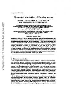
The answer to this question was found in (Polnikov et al, 2003) where the calculation of values of C d were executed with the use of the DBL-model described earlier in subsection 4.4. Results of these calculations for different values of wave age, А, and different laws for the spectrum tail fall of the kind of (7.10) are presented in Fig. 14. Analysis of the results shown in Fig. 14 permits to draw the following conclusions. 1) The scattering of friction coefficient values is secured by the physics of wind-wave interaction process. The value of C d is determined not only by the local wind speed, W, and the current value of wave age, А, but by the shape of tail of 2D-spectrum for wind

53   

waves, S (σ , θ ) , too. That explains the wide range for variability of C d , realizing in experimental observations. 2) When the falling laws for the spectrum tail are faster than fifth order in frequency, one may expect the decreasing C d with decreasing the value of А. This effect is frequently observed in experiments (for references, see Polnikov et al, 2003). But for a more weak dependence of the spectrum tail on frequency, it is probable a slow increasing the value of C d in the course of wave development, which can finish itself by fixing the final value of coefficient, growing with the growth of wind speed, W. Consequently, to distinguish the real dependencies C d (A, u*) , it needs to know (or to calculate) the high frequency tail for 2-D wind wave spectrum, the shape of which is determined by numerous factors including an impact of the surface currents, as well. 3) A simple regression dependence of C d on parameters of the system considered, alike W and A, frequently used in the wave modeling practice (including WAM and WW), is the too rough approximation. Such a kind dependence should be determined by means of the DBL-model, i.e. by means of more elaborated wind wave models (of fourth generation).

Thus, taking into account that the main parameters for a wind profile in the ABL (see formulas 4.28) are calculated with the model of DBL (i.e. without attracting the hypotheses of logarithmic wind profile), one may state that just the presence of the DBL-block in a model leads to appearance a new quality of the latter. This new quality permits to solve the applied tasks for wave forecast and atmosphere circulation with more accuracy and completeness. To the completeness of consideration, we say several words about redistribution of turbulent and wave components of the vertical momentum flux in the ABL. Numerical estimations of the profile τ w (z), made with the DBL-model said above, show that at the mean air-sea surface, the ratio of components τ t and τ w of the total momentum flux, τ , has a meaning of the following order

τ t (0) ≅ 0.5 – 0.6 , τ w (0)

(7.11)

where the value z = 0 means a mean level of the waving surface. Such a kind redistribution for the components of τ leads to a disturbance of the standard logarithmic profile for wind speed, which depends on the wave state. By other words, the use of the standard logarithmic profile for wind speed and estimation of the roughness height z 0 with formula (4.28) is the rough approximation to the real situation. Consideration of this issue in more details needs a separate research. 7.2.2. Estimation of acoustic noise intensity dependence on the wind speed. One of important practical task is an estimation of acoustic noise level produced by the air bubbles origin in the WUL due to wave crests breaking. In particular, it is very desirable to know the dependence of bubble noise intensity on the wind speed. Estimation of relative integral rate of wave energy dissipation, DRE , defined by

DRE = DE / Ef p

(7.12)

permits to give a theoretical solution of the question posed. Here, DE is the integral rate of dissipation given by (7.7), E is the total wave energy (7.4), and fp is the peak frequency. In Polnikov(2009) such estimations were done in a series of simplest cases. It was found that typical value of DRE is of the order of

54   

DRE ≈ 0,001

,

(7.13)

what leads to the following solution of the problem posed. Let us rewrite the formulas derived in Tkalich&Chan(2002), where the physical model for acoustic noise of the bubble layer in WUL was constructed. In this paper, it is shown that under certain assumptions, the intensity of bubble noise, Ia , is described by the ratio

I a = CT R (W , H S ) ⋅ ( f r / f 0 ) −2 ,

(7.14)

where CT is the theoretical coefficient, R (W , H S ) is the radius of bubble cloud as a function of the local wind speed, W, and significant wave height, H S ; ( f 0 / f r ) 2 is the non-dimensional frequency for the bubble acoustic oscillations, depending on a structure of the cloud. Further it is significant only that Ia is linearly dependent on the cloud radius, R(W), the value of which contains a whole information about the wind speed determining the dependence sought. In Tkalich&Chan(2002), it was shown that the radius value, R (W , H S ) , is linearly dependent on the rate of wave energy dissipation in accordance with the ratio R (W , H S ) = cb c t

DE Bh

.

(7.15)

Here DE is the rate of energy income into the WUL due to wave energy dissipation, cb ~ (0.3 − 0.5) is the empirical coefficient defining the fraction of value for DE spent to the bubble cloud origin, ct ≈ 0.5 is the fraction of DE spent to the turbulence production in the WUL. B is the void fraction, and h is the characteristic depth of the bubble cloud (mass center). Values of cb and B are determined from experimental observations, and the value of ct can be estimated theoretically with the physical models of DBL, discussed above in Sec. 3. Further we will suppose that the values mentioned have a weak dependence on wind. In such a case, the sought dependence takes the kind, I a (W ) ∝ R(W ) , so it can be determined on the basis of calculation for DE (W ) and on physical models describing the dependence h(W ) . According to definition (7.12), the dependence DE (W ) can be found from calculations for the magnitude E(W) and from tabulated rate of the non-dimensional dissipation for wave energy, DRE(W). In general case, for the wind field prescribed, this task is solved by means of numerical simulation a wind wave spectrum evolution at the fixed point in the basin under consideration. But in the simplest case of constant and homogeneous wind field, the sought dependences can be ~ obtained with the use of result (7.13) and well known empirical dependences of E (W ) for the fully developed sea, (6.4), (6.5). Let us consider the fully developed sea. In such a case, with the account of ratios (7.12) and (7.13), one may write DE (W ) = 0.001 E w (W ) f p (W ) .

(7.16)

As far as for the fully developed sea, dependences E w (W ) and f p (W ) are given by the well known ratios (6.4), (6.5), we have

E w ≈ 3 ⋅10 −3 W 4 g 2

(7.17)

f p ≈ g /W 2π .

(7.18)

and

55   

Then, under the assumption of the lack of dependence B(W ) , for the acoustic noise intensity due to bubbles we have

I a (W ) ∝ W 3 / h(W ) .

(7.19)

Thus, in the case considered, the final result is determined by the model for a depth of the bubbles cloud center, h(W) . There are possible the following cases here. I. In the case of weak wave sea, the assumption that h = const is quite reasonable, due to small dependence of any mechanical parameters for WUL on the wind (including the bubble cloud deepening). In such a case, the dependence I a (W ) is determined by the ratio Ia ~ W 3 .

(7.20)

II. In the case of rather visible waves which are far from their extreme development, it is widely used the following empirical formula (see Tkalich&Chan, 2002) h ≈ 0.35HS

,

(7.21) 1/2

where HS is the significant wave height. With the account of definition HS =1,4(E) , the sought dependence (7.19) takes the kind Ia ~ W .

(7.22)

III. And finally, in the case of high winds and fully developed sea, it is more reasonable to put that the bubble cloud depth is linearly related to the radius of the cloud, i.e. h ∝ R . Under such an assumption and with the account of ratios (7.16)-(7.18), the solution of equation (7.15) reads h(W ) ∝ W 3 / 2 .

(7.23)

Consequently, in this case, the sought dependence takes the kind Ia ~ W 3 / 2 .

(7.24)

It is interesting to note that all three types of dependences I a (W ) , i.e. formulas (7.20), (7.22) and (7.24), do well correspond to generalized observation data presented in Tab. 5, which is Table 5. Empirical estimations for dependence I a (W ) . Wind speed (m/s)

Dependence I a (W )

Wave state

I

5 15 m) for 5 different regions of the Atlantic. 5. Making electronic maps of wave heights distributions for the extraordinary events in the whole Atlantic (i.e. wind speed is more 30 m/s, or wave heights are of H s > 15m). 7.3.2. Method of study Having a modern wind wave model (for example, WAM with the optimized source function, as it was done in Polnikov et al, 2008), one could make numerical simulations of wave evolution in the whole Atlantic Ocean for the period of 20 years, to get a good statistics of waves. The proper wind field data are available for us on the space grid 10x10 with the time discrete of 3h. Method of the wave climate study includes the following actions. A. One makes a spatial partition of the whole Atlantic into 5 parts having, for example, the following boundaries: (X- longitudes, Y – latitudes) 1. Western part of the North Atlantic (WNA): 100W < X < 40W,

20N < Y < 78N;

2. Eastern part of the North Atlantic (ENA):

40W < X < 20E,

20N < Y < 78N;

3. Tropical part of the Atlantic (TA):

100W < X < 20 E,

20S < Y < 20N;

4. Western part of the South Atlantic (WSA): 100W < X < 40W,

78S < Y < 20S;

5. Eastern part of the South Atlantic (ESA):

78S < Y < 20S.

40W < X < 20E,

B. One introduces 3 reference values of significant wave height, H s , which distinguish description of different meteorological events: • Ordinary waves heights (with H s > 3m);                                                              6  Partition means fixing the numbers of events in the following 5 regions: Western part of North Atlantic,  Eastern  part  of  North  Atlantic,  Tropical  (near‐equatorial)  part  of  Atlantic,  Western  part  of  Southern  Atlantic, and Eastern part of Southern Atlantic.

58   

• Extreme wave heights ( H s > 10m); • Extraordinary wave heights ( H s > 15m). C. In each region of the Atlantics, description of the following events is of interest: a) Distribution in space and time of the mechanical energy accumulated in atmosphere, E A (t ) , (wind) and in ocean, E w (t ) , (wind waves) (task 1). Atmosphere energy time history, E A (t ) , is calculated by the formula

E A (t ) = ΔS ∑ i , j ,n

ρa 2

Wi ,3j (tn )Δtn

(7.25)

where ρ a is the air density, and Wi , j (t ) is the wind at the standard horizon (z = 10m) and at each space-time grid points, (i,j) and time moment tn. Each term under the sum in (7.25) is the density of the kinetic energy flux over a unit of the surface, ΔS . Wind waves energy analog is calculated by the formula

E w (t ) = ΔS ∑ i, j

ρwg 16

H i2, j (t )

(7.26)

where ρ w is the water density. Each term under the sum in (7.26) is the density of the mechanical energy of waves over unit of the surface. In addition to the said, it is very interesting to calculate a corresponding distribution in space and time of the rate of mechanical energy input into waves from wind, I w ( R, T ) , and the mechanical energy dissipated by wind waves, Dw ( R, T ) . These values are calculated by the use of the proper source function terms, In and Dis, applied in the model under consideration. Proper formulas are as follows ⎡⎛ ⎞⎤ I w ( R, T ) = ∑ Δt ⎢⎜⎜ ∑ ΔS ∫ In(ω, θ , Wi , j , Si , j )dθdθ ⎟⎟⎥ (7.27) n∈T ⎠⎦⎥ ⎣⎢⎝ i , j∈R

⎡⎛ ⎞⎤ Dw ( R, T ) = ∑ Δt ⎢⎜⎜ ∑ ΔS ∫ Dis(ω, θ , Wi , j , Si , j )dθdθ ⎟⎟⎥ (7.28) n∈T ⎠⎦⎥ ⎣⎢⎝ i , j∈R with the evident sense of notations. Necessity to separate calculation of the mechanical energy input I w ( R, T ) , in addition to atmospheric and wave energy distributions, E A ( R, T ) and E w (R, t ) , is provided by the fact that not all the energy I w ( R, T ) , supplied by the wind to waves, is got, as far as a some part of it is dissipated by waves into the water upper layer. Calculation of the dissipated energy, Dw ( R, T ) , is interesting to check the balance of the kind B ={ I w ( R, T ) - Dw ( R, T ) - E w ( R, t ) } (7.29) Positive sing of the magnitude B means a presence of a wave energy divergence for the region considered (due to a wave energy advection), but the negative sing does convergence. For the whole world ocean (or a large-scale space) the total balance B should be close to zero. One of the points of interest is to check this fact. Study of these values is important for understanding of the mechanical energy exchange between atmosphere and ocean and their climate variability. 20-years historical series of such values could be needed for estimation of the wave climate variability in time and space. b) Statistics of the maximum waves. It includes seasonal, annual and total (20-years) histogram of the maximum wave heights, obtained by simulations of wave evolution for 20 years

59   

(task 2). This information is important for understanding a regional distribution of wind waves by their strength. c) Registration of domains with the extreme waves in each region of the Atlantic, and making comparison the numbers of events among the regions (task 3). This information is important for determination of the most dangerous region in the Atlantic. d) Registration of the extreme wave’s duration in the regions (task 3). This information gives more details of the previous study (task 4). It is important for evaluation of the time variability of the extreme events. e) Making the atlas of maps and seasonal-annual statistics of the extraordinary waves (number of the events in each region) (task 5). This is important for understating of the extraordinary events distribution among regions for the long period. There is no map of such a kind, and for this reason they are of great scientific and practical interest. The said above does clarify the purpose and the method of executing the project proposed. We sure that the work drafty described in this subsection will be very fruitful in many aspects.

60   

8. REFERENCES Ardhuin, F., Chapron, B., Elfouhaily, T. J Phys Oceanogr. 2004, 34, 1741-1755. Babanin, A.V. Acta Physica Slovaca 2009 , 59, 305-535. Babanin ,V.A., Young, I.R., Banner, M.L. J Geophys Res. 2001, 106C, 11659–11676. Banner, M.L., Young, I.R. J. Phys. Oceanogr. 1994, 24, 1550-1571. Banner, M.L., Tian, X. J Fluid Mech. 1998, 367, 107-137. Chalikov, D.V. Boundary Layer Meteorology 1980, 34, 63-98. Chalikov, D., Sheinin, D. Advances in Fluid Mechanics 1998, 17, 207 – 222. Drennan, W.M., Kahma, K.K., Donelan, M.A. Boundary-Layer Meteorology 1999, 92,. 489-515. Donelan, M.A., Dobson, F.W., Smith, S.D., et al. J Phys Oceanogr. 1993, 23, 2143-2149. Donelan, M. A. Coastal and Estuarine Studies 1998, 54, 19-36. Donelan, M.A. Proc. ECMWF Workshop on Ocean Wave Forecasting, Reading, UK, ECMWF. 2001, 87–94. Efimov, V.V., Polnikov, V.G. Oceanology 1985, 25, 725-732 (in Russian). Efimov, V.V., Polnikov, V.G. Numerical modelling of wind waves. Naukova dumka Publishing house. Kiev. UA. 1991, 240 (in Russian). Fomin, V.N., Cherkesov, L.V. Izvestiya, Atmospheric and Oceanic Phys. 2006, 42, 393-402 (in Russian). Hasselmann, K. Shifttechnik 1960, 7, 191-195 (in German). Hasselmann, K. J Fluid Mech. 1962, 12, 481-500. Hasselmann, K. Boundary Layer Meteorology 1974, 6, 107-127. Hwang, P. A., Wang D. W. Geophys Res Letters 2004, 31, L15301, doi:10.1029/2004GL020080. Janssen, P.E.A.M. J Phys Oceanogr. 1991, 21, 1389-1405. Kitaigorodskii, A., Lumley, J.L. J. Physical Oceanography 1983, 13, 1977-1987. Komen, G.L., Cavaleri, L., Donelan, M., et al. Dynamics and Modelling of Ocean Waves, Cambridge University Press. UK. 1994, 532 p. Krasitskii, V.P. J Fluid Mech. 1994, 272, 1-20. Lavrenov, I.V., Polnikov, V.G. Izvestiya, Atmospheric and Oceanic Phys. 2001, 37, 661-670 (English transl.). Makin, V.K., Kudryavtsev, V.N. J Geophys Res 1999, 104, 7613-7623. Miles, J.W. J. Fluid Mech. 1960, 7, 469-478. Monin, S.A., Krasitskii, V.P. Phenomena on the ocean surface. Hydrometeoizdat. Leningrad. RU. 1985, 375p. Monin, A.S., Yaglom, A.M. Statistical Fluid Mechanics: Mechanics of Turbulence.. The MIT Press, Cambridge, Massachusets, and London, UK. 1971, v.1, 769 p. Pedloskii. J. Geophysical Fluid dynamics. Springer Verlag. N.Y. 1984, V.1. 350 p. Phillips, O.M. J. Fluid Mech. 1957, 2, 417-445.

61   

Phillips, O.M. Dynamics of the Upper Ocean. Second ed., Cambridge University Press, UK. 1977, 261 pp. Phillips, O.M. J. Fluid Mech. 1985, 156, 505-631.

Plant, W.J. J Geophys Res. 1982, 87, 1961-1967. Polnikov, V.G. Izvestiya, Atmospheric and Oceanic Physics, 1991, 27, 615-623 (English transl.). Polnikov, V.G. Proceedings of Air-Sea Interface Symposium, Marseilles, France. Marseilles University. 1994, 227-282. Polnikov, V.G. The study of nonlinear interactions in wind wave spectrum. Doctor of Science dissertation. Marine Hydrophysical Institute of NASU. Sebastopol. UA. 1995, 271p (in Russian). Polnikov, V.G. Nonlinear Processes in Geophysics 2003, 10, 425-434. Polnikov, V.G. Izvestiya, Atmospheric and Oceanic Physics 2005, 41, 594–610 (English transl.). Polnikov, V.G. Nonlinear theory for stochastic wave field in water. LENAND publishing house. Moscow. RU. 2007, 404p (in Russian). Polnikov, V.G. Izvestiya, Atmospheric and Oceanic Physics 2009a, 45, 346–356 (English transl.). Polnikov, V.G. Izvestiya, Atmospheric and Oceanic Physics 2009b, 45, 583–597 (English transl.). Polnikov, V.G., Dymov, V.I., Pasechnik, T.A., et al. Oceanology 2008, 48, 7–14 (English transl.). Polnikov, V. G., Farina, L. Nonlinear Processes in Geophysics 2002, 9, 497-512. Polnikov, V.G., Innocentini, V. Engineering Applications of Computational Fluid Mechanics 2008, 2, 466-481. Polnikov, V.G., Tkalich, P. Ocean Modelling 2006, 11, 193-213. Polnikov, V.G., Volkov, Yu.A., Pogarskii, F.A. Nonlinear Processes in Geophysics 2002, 9, 367-371. Polnikov, V.G., Volkov Yu. A., Pogarskii, F.A. Izvestiya, Atmospheric and Oceanic Phys. 2003, 39, 369-379 (English transl.). Proceedings of the symposium on the wind driven air-sea interface. Ed. by M. Donelan. The University of Marseilles, France. 1994, 550p. Proceedings of the symposium on the wind driven air-sea interface. Ed. by M. Banner. The University of New South Wales, Sydney, Australia. 1999, 452p. Qiao, F., Yuan, Y., Yang, Y., et al. Geophysical Research Letter 2004, 31, L11303, doi: 10.1029/2004GL019824. Rodriguez, G., & Soares, C.G. 1999 Uncertainty in the estimation of the slope of the high frequency tail of wave spectra. Applied Ocean research. 21, 207-213. Snyder, R.L., Dobson, F.W., Elliott, J.A., Long, R.B. J Fluid Mech. 1981, 102, 1-59. Stokes, G.G. Transaction of Cambridge Phys Soc. 1947, 8, 441 -455.

The SWAMP group. Ocean wave modelling. Plenum press. N.Y. & L. 1985, 256 p. The WAMDI Group. J Phys Oceanogr. 1988, 18, 1775-1810. The WISE group. Progress in oceanography 2007, 75, 603-674.

62   

Tkalich, P., Chan, E.S. J Acoustical Society of America 2002, 112, 456-483. Tolman, H.L., & Chalikov. D.V. J Phys Oceanogr. 1996, 26, 2497-2518. Yan, L. Report No. 87-8. 1987. Royal Dutch Meteorological Inst., NL. 20p. Young, I. R., Babanin, A. V. J Phys Oceanogr. 2006, 36, 376–394. Zakharov, V.E. Applied mechanics and technical physics 1968, 2, 86-94 (in Russian) Zakharov, V. E. Izvestiya VUZov, Radiofizika 1974, 17, 431-453 (in Russian). Zakharov, V.E., Korotkevich, A.O., Pushkarev, A., Resio, D. Phys Rev Letters 2007, 99, 16-21 Zaslavskii, M.M., Lavrenov, I.V. Izvestiya, Atmospheric and Oceanic Phys. 2005, 45, 645-654 (in Russian).