Available online at www.sciencedirect.com Available online at www.sciencedirect.com
Procedia Engineering
Procedia Engineering 00 (2011) 000–000 Procedia Engineering 29 (2012) 1979 – 1983 www.elsevier.com/locate/procedia
2012 International Workshop on Information and Electronics Engineering (IWIEE)
Numerical Research on Stochastic Duffing System Mingyu Wanga*, Fengying Sua a
School of Information,Xi’an University of Finance and Economics,Xi’an 710100 ,China
Abstract In this paper, the numerical simulation method is applied to investigate the nonlinear stochastic bifurcation systems. In order to obtain a better understanding of the relationship between the Lyapunov exponents and stochastic bifurcation, the Duffing system under stochastic external excitations is examined by way of the stochastic process simulation.The simulation results are compared with the results of some other analytical methods, such as the stochastic averaging method, the perturbation method and the Laplace asymptotic evaluation method. It is shown that these analytical methods are all valid if the intensity of the noise is small. And the numerical method can be applied to the case of arbitrary noise intensity.
© 2011 Published by Elsevier Ltd. Selection and/or peer-review under responsibility of Harbin University of Science and Technology Open access under CC BY-NC-ND license. Keywords: nonlinear stochastic systems; Duffing system; Lyapunov exponents; numerical simulation
1. Introduction Consider the deterministic dynamic system described by following equation
& f ( x, α ), x(0)= x0 ∈ R n x=
(1)
= α (α1 , α 2 ,Lα r )T ∈ R r is parameter vector, and f is a n-dimension nonlinear function, where
suppose α is disturbed by noise, then the corresponding dynamical equation can be described by the stochastic differential equation
*
* Corresponding author. Tel.: +86-029-81556311. E-mail address:
[email protected].
1877-7058 © 2011 Published by Elsevier Ltd. Open access under CC BY-NC-ND license. doi:10.1016/j.proeng.2012.01.247
1980 2
Mingyu Wang Fengying Su /Engineering Procedia Engineering 29 (2012) 1979 – 1983 Wang MYand Su FY/ Procedia 00 (2011) 000–000
x& = f ( x, α + σξ (t )), x(0) = x0 ∈ R n where ξ (t ) is r-dimension stochastic process.
(2)
& A( xs (t ), ξ (t ))v, v(0)= v0 ∈ R n v=
(3)
When the stochastic system (2) is at the condition of edge from one steady movement change into another steady movement, the small changes of the control parameters of the system can produce effect, so it is necessary to study the bifurcation problem of the nonlinear stochastic system first. In discussion of a deterministic system, we can use the changes of the topology for the phase track to describe the bifurcation phenomena. But the formulation of the topology for the phase track is no longer fit for the stochastic system. The stochastic response behavior of the process should be described by the probability density function. The structure changes of the corresponding steady-state probability density function can be used to describe the stochastic bifurcation phenomena [1,2,3]. Let xs be a steady solution of (2), in order to discuss the stability of solution and the random bifurcate problem, we get the following stochastic differential equations
where Jacobi matrix
⎛ ∂f A( x, ξ ) = ⎜ i ⎜ ∂x ⎝ j
⎞ ⎟⎟ ⎠ n× n
(4)
the exponential growth rate of the solution of (3) is determined by the following Lyapunov exponents in probability 1:
1 n →∞ t
λ (v0 ) = lim ln v(t , v0 )
(5)
The theory of Lyapunov exponents is an important tools in dynamical systems, starting with the pioneer work of Liao [4] and Oseledec [5]. We refer to [6,7,8] for the general theory of the Lyapunov exponents and its recent developments. One of the key problems of the research of stochastic bifurcation is how to calculate the largest Lyapunov exponents for nonlinear stochastic systems. The calculation of the largest Lyapunov exponent was provided by Khasminskii [9] at first. When the disturbance is small, the approximation of the largest Lyapunov exponent can be obtained by stochastic averaging method [10] or the perturbation method [11] . We adopt the numerical simulation method to calculate the largest Lyapunov exponent of the nonlinear stochastic systems. 2. Numerical calculation of the Lyapunov exponent of the stochastic system We still consider the stochastic dynamic system described by the equation (2). (2) x& = f ( x, α + σξ (t )), x(0) = x0 ∈ R n for convenience, we assume ξ1 (t ) , ξ 2 (t ) , … , ξ r (t ) are independent standard normal white noise process, and the corresponding linearized system is
& Av, v(0)= v0 ∈ R n v= (3) If σ = 0 , then the system is deterministic. We will use the numerical simulation method to calculate
the Lyapunov exponents, especially the largest Lyapunov exponent of the stochastic system.
1981 3
Mingyu Wang and Su / Procedia Engineering 29 (2012) 1979 – 1983 Wang MYFengying Su FY / Procedia Engineering 00 (2011) 000–000
We know, at the given moment t0 , random process ξi (t ) equivalent as a random variable. We imagine in a "transient", ξi (t0 ) value for random numbers, then in that "transient", the response of the system (2) and its linearized system can be obtain by numerical simulation method. If the random process is ergodic, and the random numbers can be given much enough, then the Lyapunov exponents can be calculated by numerical simulation method. Consider nonhomogeneous filter Poisson process
= x(t )
N (t )
∑ Y δ (t − t ) n =1
n
n
(6)
where N(t) is a Poisson process with arrival rate v, Yn is an i.i.d. sequence of random variables, and the mean value E Yn = 0 , and independent to N(t). δ (t − tn ) is Diracδfunction, so the mean value and covariance function of X(t) are respectively as
μ X (t ) = 0
(7)
= K XX (t2 , t1 ) E (Y ) v(t1 )δ (t2 − t1 ) 2
= I (t1 )δ (t2 − t1 )
(8)
if Poisson process is homogeneous, i.e. arrival rate v(t) is the constant, then
K XX (t= I (t1 )δ (t2 = − t1 ) R XX (t2 , t1 ) 2 , t1 )
(9)
So X(t) is white noise. If v(t) is big enough, then the distribution of white noise process is normal. Therefore the continuous white noise process can be instead of the homogeneous Poisson pulse process. Let the state equation of the random dynamic system (2) be
⎧ x&1 = x2 ⎨ ⎩ x&2 = F ( x1 , x2 , t ; α )
(10)
the corresponding linearized system be
⎧ v&1 = v2 (11) ⎨ ⎩v&2 = A( x1 , x2 , t ; α )v2 where α of (10) and (11) is the abbreviations of α + σξ (t ) . So the calculation process of Lyapunov
exponents is similar to the deterministic system. Just in the numerical simulation process, input a random number within the integrating process, i.e. in small enough time intervals input a random number with normal distribution, so as to
α =i α + σξi
(12)
3. Calculation example To investigate whether the algorithm is valid, we will use the algorithm to calculate the Lyapunov exponents of the Duffing system under stochastic external excitations and the results are compared with
1982 4
Mingyu Wang Fengying Su /Engineering Procedia Engineering 29 (2012) 1979 – 1983 Wang MYand Su FY/ Procedia 00 (2011) 000–000
the results of some other analytical methods, such as the stochastic averaging method, the perturbation method and the Laplace asymptotic evaluation method. Consider the Duffing system described by following equation
&& x + cx& + x + x 3 = F cos(bt )
(13) System (13) may occur symmetrical rupture bifurcation, period-doubling bifurcation and even chaos movement when external excitations change. Now let c=0.1, b=0.95, and amplitude F is disturbed by noise, then the corresponding dynamical equation can be described by following equation
&& x + cx& + x + x 3 = ( F + σξ (t )) cos(bt )
(14)
where ξ(t) is unit normal white noise process. 2 Fig. 1 and Fig. 2 are the curve of the largest Lyapunov exponent with the change of F .
Fig. 1 The largest Lyapunov exponent with σ=0
Fig. 2 The largest Lyapunov exponent with σ=0.1
Fig 3 and Fig 4 show that the Lyapunov exponent has cardinally identical trends in the circumstances of the less noise and no noise intensity. But it is different for the amplitude of the scope of different excitation effect.
Fig. 3 The largest Lyapunov exponent with σ=0.1
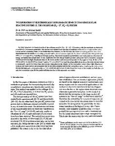
Fig. 4 The largest Lyapunov exponent with σ=0.1
Fig. 3 is the partial enlargement of the figure 4 when F2 changes in 1126~1128. It can be seen that the effect of noise is to move the bifurcation point from 1126.795 to 1126.25. And the stability and trend of the system before or after bifurcation is consistent with no noise. But when F2 is in other variation area, noise not only can make drift bifurcation point occurs, the system can be made from stable to unstable, such as F2 changes in nearby 1136 (see Fig. 4). Or the system is made from unstable into stable, such as F2 changes in nearby 1139.65 F2 (see Fig. 5).
Mingyu Wang and Su / Procedia Engineering 29 (2012) 1979 – 1983 Wang MYFengying Su FY / Procedia Engineering 00 (2011) 000–000
Fig. 5 The largest Lyapunov exponent with σ=0.1
The similar conclusions can also be obtained if we study the incentive frequency of noise disturbance. 4. Conclusion For stochastic system, we can not determine the precise value of the Lyapunov exponents. So the stochastic averaging method, the perturbation method and the Laplace asymptotic evaluation method can usually be used to get approximate value of the Lyapunov exponents. But these method are no longer valid if the intensity of the noise is not small. In this paper, the numerical method for computing the Lyapunov exponents of the nonlinear stochastic systems is presented by way of the stochastic process simulation. It is shown that the numerical method can be applied to the case of arbitrary noise intensity. References [1] Horsthemake, W and Lefever, R. Noise-Induced Transitions. Berlin: Springer-Verlag. 1984 . [2] Zhu Weiqiu. The Probability Density Functions of the Stationary Response of Certain Classes of Nonlinear Systems to Stochastic Excitation. Acta Mechanica Sinica. 1991; 23(1):92-102 (in Chinese). [3] Rong Haiwu, Wang Xiangdong, Xu Wei et al. On double-peak probability density functions of a Duffing oscillator under narrow-band random excitations. Acta Physica Sinica. 2005; 54(6):2557-2561 (in Chinese). [4] Liao S T. Certain ergodic preperties of a differential systems on a compact differentiable manifold. Acta Sci Natur Univ Pekinensis. 1963; 9:241-265, 309-326. [5] Oseldec VI. A Multiplicative Ergodic Throrem Lyapunov Characteric Numbers for Dynamical Systems. Trans. Moscow.Math. Soc., 1968; 19:197-231. [6] Arnold L. Lyapunov Exponents of Nonlinear Stochastic Systems. Proc. IUTAM, Nonlinear Stochastic Dynamic Engineering Systems. Innsbruck, Austria. F. Ziegler, G.I. Schuller (Eds.), Berlin: Springer-Verlag. 1987; 181-201. [7] Barreira L, Pesin Y. Lyapunov Exponents and Smooth Ergodic Theory. University Lecture Series 23, Providence, RI: Amer Math Soc, 2002. [8] Zhu Yujun, Zhang Jinlian. Lyapunov Exponents for continuous random transformations. Science China Math, 2010; 53(2):413-424. [9] Khasminskii R Z. Necessary and sufficient conditions for the asymptotic stability of linear stochastic systems. Theory Prob. Appl., 1967; 12:144-147. [10] Stratonovitch R L. Topics in the Theory of Random Noise, Gordon and Breach, Vol.1, 1963, Vol.2, 1967. [11] Arnold L Papanicolaou G and Wihstutz V. Asymptotic Analysis of the Lyapunov Exponent and Rotation Number of the Random Oscillator and Applications. SIAM J. Appl. Math. 1986; 46(3):427:450.
1983 5