numerical simulation of a mathematical traffic flow model based on a ...

Journal of Bangladesh Academy of Sciences, Vol. 34, No. 1, 15-22, 2010

NUMERICAL SIMULATION OF A MATHEMATICAL TRAFFIC FLOW MODEL BASED ON A NONLINEAR VELOCITY-DENSITY FUNCTION M. H. KABIR, M. O. GANI and L. S. ANDALLAH Department of Mathematics, Jahangirnagar University, Savar, Dhaka, Bangladesh ABSTRACT A mathematical macroscopic traffic flow model known as Lighthill, Whitham and Richards (LWR) model appended with a closure nonlinear velocity-density relationship yielding a quasilinear first order (hyperbolic) partial differential equation as an initial boundary value problem (IBVP) was considered. The traffic model IBVP by finite difference method which leads to a first order explicit upwind difference scheme was discretized. Computer programs for the implementation of the numerical scheme and perform numerical experiments in order to verify some qualitative traffic flow behaviour for various traffic parameters were developed.

Key words: Numerical simulation, Trafic flow model, Nonlinear velocity, Density function INTRODUCTION Nowadays traffic flow and congestion is one of the main societal and economical problems related to transportation in industrialized countries. Traffic congestion is one of the greatest problems in Bangladesh like some other countries of the world. In this respect, countries managing traffic in congested networks requires a clear understanding of traffic flow operations. The aims of this analysis are principally represented by the maximization of vehicles flow, and the minimization of traffic congestions, accidents and pollutions etc. Macroscopic fluid-dynamic model which is characterized by representations of traffic flow in terms of aggregate measures such as flux, space mean speed, and density was focused. In this paper (Section 2), we consider a macroscopic traffic model developed first by Lighthill and Whitham (1955) and Richard (1956) shortly called LWR model based on Habermann (1977), Klar (1996). As presented in Kabir (2006), we study finite difference method for first order non-linear PDE from Leveque (LeVeque 1992), Larsson and Thomee (Larsson and Thomce 2005), Morton and Mayers (Morton and Mayers 1995) and based on these, we develop a finite difference scheme for our traffic flow model as an (IBVP) which has been presented in Section 3. We develop computer programming code for the implementation of the numerical scheme and perform numerical experiments in order to verify some qualitative traffic flow behaviour for various traffic parameters. In Section 4 we present the numerical results.

16

KABIR et al.

Macroscopic model of traffic flow The macroscopic traffic model developed first by Lighthill and Whitham (1955) and Richard (1956) shortly called LWR model is most suitable for correct description of traffic flow; details can be seen in (Haberman 1977). In this model, vehicles in traffic flow are considered as particles in fluid: further the behaviour of traffic flow is modeled by the method of fluid dynamics and formulated by hyperbolic partial differential equation (PDE). The macroscopic traffic flow model is used to study traffic flow by collective variables such as traffic flow rate (flux) q(x,t ), traffic speed V (x, t ) and traffic density ρ (x,t ), all of which are functions of space, x ∈ ℜ and time, t ∈ ℜ + . The wellknown LWR model is formulated by employing the conservation equation

∂ρ ∂q(ρ ) + =0 ∂t ∂x

(2.1)

A non-linear velocity-density relationship of the form was used

⎛

2 ⎛ ρ ⎞ ⎞⎟ ⎟⎟ ⎝ ρ max ⎠ ⎟⎠

V (ρ ) = Vmax ⎜1 − ⎜⎜ ⎜ ⎝

then the flux is of the form

⎛ ⎛ ρ ⎞2 ⎞ ⎟ ⎟ q(ρ ) = ρv( ρ ) = ρ .Vmax ⎜1 − ⎜⎜ ⎜ ⎝ ρ max ⎟⎠ ⎟ ⎝ ⎠ and leads to formulate a nonlinear first order hyperbolic partial differential equation (PDE) of the form

⎛ ρ 2 ⎞⎞ ∂ρ ∂ ⎛⎜ .Vmax ⎜⎜1 − 2 ⎟⎟ ⎟ = 0 ρ + ⎟ ∂t ∂x ⎜⎝ ⎝ ρ max ⎠ ⎠

(2.2)

Analytical and numerical methods for traffic flow model The non-linear PDE is considered as an initial value problem (IVP) of the form

⎛ ρ 2 ⎞⎞ ∂ρ ∂ ⎛⎜ ρ .Vmax ⎜⎜1 − 2 ⎟⎟ ⎟ = 0 + ⎟ ∂t ∂x ⎜⎝ ⎝ ρ max ⎠ ⎠ ρ (t0 , x ) = ρ 0 (x ) The IVP (3.1) can be solved by the method of characteristics as follows: The PDE in the IVP (3.1) may be written as

∂ρ ∂q(ρ ) =0 + ∂x ∂t

(3.1)

NUMERICAL SIMULATION OF A MATHEMATICAL TRAFFIC FLOW

17

where

⎛ ρ2 q(ρ ) = ρ .Vmax ⎜⎜1 − 2 ⎝ ρ max

⇒

∂ρ dq ∂ρ + =0 ∂t dρ ∂x

⇒

⎛ 3ρ 2 ∂ρ + Vmax ⎜⎜1 − 2 ∂t ⎝ ρ max

⎞ ⎟⎟ ⎠

⎞ ∂ρ ⎟⎟ =0 ⎠ ∂x

Now

dρ ∂ρ ∂ρ dx = + =0 ∂t ∂x dt dt

(3.2

where

⎛ 3ρ 2 dx = Vmax ⎜⎜1 − 2 dt ⎝ ρ max

⎞ ⎟⎟ ⎠

(3.3)

Equations (3.2) and (3.3) give

⎛ 3ρ 2 ⎞ x(t ) = Vmax ⎜⎜1 − 2 ⎟⎟ t + x 0 ⎝ ρ max ⎠

(3.4)

which is known as the characteristics curve of the IVP (3.1). Now from equation (3.2) we have

dρ =0 dt

∴ ρ ( x, t ) = c

(3.5)

(

)

Since the characteristics through ( x, t ) also passes through x 0 , 0 and ρ ( x, t ) = c is constant on this curve, so we use the initial condition to write

c = ρ (x, t ) = ρ (x 0 , 0 ) = ρ 0 (x 0 )

(3.6)

Equation (3.5) and (3.6) yield

ρ (x, t ) = ρ 0 (x 0 )

(3.7)

Using equation (3.4), (3.7) takes the form

⎛

⎛

⎝

⎝

ρ (x, t ) = ρ 0 ⎜⎜ x − Vmax ⎜⎜1 −

3ρ 2 ⎞ ⎞⎟ ⎟⎟t 2 ⎟ ρ max ⎠ ⎠

(3.8)

This is the analytic solution of the IVP (3.1) which is in implicit form. Moreover, in reality it is very difficult to formulate ρ 0 ( x) from data. Therefore, there is unavoidable to

17

18

KABIR et al.

use numerical methods for solving the IVP (3.1) as an initial boundary value problem (IBVP), which is also appended with boundary condition. Therefore, we study finite difference method for first order non-linear PDE presented in Leveque (1992), Larsson and Thomee (2005), Morton and Mayers (1996) and based on this, in the following, we investigate a finite difference scheme for our considered traffic flow model as an (IBVP).

⎛ ⎛ ρ ∂ ⎛⎜ ∂ρ ρ .V max ⎜ 1 − ⎜⎜ + ⎜ ⎜ ⎝ ρ max ∂t ∂x ⎝ ⎝

⎞ ⎟⎟ ⎠

2

⎞⎞ ⎟ ⎟ = 0 ; x ∈ (a , b ) ; t ∈ (0, T ) ⎟⎟ ⎠⎠

with initial condition ρ(x, 0) = ρ0(x) and boundary condition ρ(a, t) = ρa(t).

(3.9)

(3.10)

Equation (3.9) may be written as

∂ρ ∂q(ρ ) + =0 ∂t ∂x

(3.11)

where

⎛ ⎛ ⎛ ρ q(ρ ) = ⎜ ρ .Vmax ⎜1 − ⎜⎜ ⎜ ⎜ ⎝ ρ max ⎝ ⎝

⎞ ⎟⎟ ⎠

2

⎞⎞ ⎟⎟ ⎟⎟ ⎠⎠

In order to develop the scheme, we discretize the space and time. The discretization

∂ρ (x, t ) of is obtained by first order forward difference in time and the discretization of ∂t ∂ρ(x, t ) is obtained by first order backward difference in space. ∂x The possible finite difference approximations for

∂ρ ∂ρ and : ∂t ∂x

Forward difference in time: From Taylor’s series we write

ρ ( x, t + h ) = ρ ( x, t ) + h ⇒ ∴

∂ρ (x, t ) h 2 ∂ 2 ρ ( x, t ) + + ... ∂t 2! ∂t 2

∂ρ (x, t ) ρ (x, t + h ) − ρ ( x, t ) = − (h ) ∂t h

∂ρ ( x, t ) ρ ( x, t + h ) − ρ ( x, t ) ≈ h ∂t

(3.12)

Similarly, backward difference in space

∂ρ ( x, t ) ρ ( x, t ) − ρ ( x − k , t ) ≈ k ∂x

(3.13)

NUMERICAL SIMULATION OF A MATHEMATICAL TRAFFIC FLOW

19

We assume the uniform grid spacing with step size h and k for time and space, respectively t n +1 = t n + h and xi +1 = xi + k . We also write

ρ in

for

ρ (x, t )

in equations (3.12) and (3.13).

Now equation (3.11) takes the form

ρ in +1 − ρ in Δt

n+

1 2

+

qin − qin−1 =0 Δxi n+

⇒ ρ in +1

1

Δt 2 n qi − qin−1 = ρ in − Δxi

[

]

(3.14)

where

⎛ ⎛ ρn q = ρ Vmax ⎜1 − ⎜⎜ i ⎜ ⎝ ρ max ⎝ n i

n i

⎞ ⎟ ⎟ ⎠

2

⎞ ⎟ ⎟ ⎠

This is the explicit upwind difference scheme for the equation (3.9). Therefore, equation (3.14) leads to the desired numerical scheme for the traffic model. Numerical simulations We have developed computer programs for the implementation of the numerical scheme and perform numerical experiments in order to verify some qualitative traffic flow behaviour for various traffic parameters as in the case of linear density-velocity relationship presented in (Andallah et al. 2008). Details can also be seen in Kabir (2006). To obtain the density profile we have used the explicit upwind difference scheme. In order to use the scheme we have made the following assumptions: ¾

We have considered a highway in a range of 10 km.

¾

We consider the number of vehicles of various points at a particular time as initial data and constant boundary ρ (0, t ) = 21 / 0.1 km

¾

We have estimated maximum density which is parameterized by ρ max in the traffic flow model. To evaluate ρ max , we have used the following equation

ρ max = max ρ (0, x ) * c For this we use the initial density for ρ (0, x ) and take c = 10 as a constant. According to focusing on some parameters we present some specific cases of traffic flow which are as follows: Case A: In this case we choose maximum speed, Vmax = 60 km/hour. We consider ρ max = 250 / km and perform numerical experiment for 6 minutes in Δt = 90

19

20

KABIR et al.

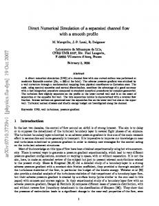
time steps (temporal grid size) for a highway of 10 km in 51 spatial grid points with step size Δx = 100 meters. We considered the initial density ρ (0, x ) as presented in Fig. 1

and the constant boundary value ρ (t ,0 ) = 21 / 0.1 km. We wanted to simulate the traffic flow for six minutes. In Fig. 2, the curve marked by solid line represents the density of car at 2 minutes, and the curve manifested as “-o-” represents the density profile at 4 minutes also the curve manifested as “-*-” represents the density profile at 6 minutes, respectively. 24

22.6

23.5

22.4 22.2 Density of Car /0.1km

23 Density of Car /0.1km

2min 4min 6min

22.5 22 21.5

22 21.8 21.6 21.4

21

21.2 20.5 20

21 0

1

2

3

4 5 6 Highway [km]

7

8

9

20.8

10

0

1

Fig. 1. Initial traffic density in 0.1 km.

2

3

4 5 6 Highway [km]

7

8

9

10

Fig. 2. Density of car for 6 minutes.

Fig. 3 represents the respective computed velocity profile according to the certain points of the highway. The velocity is computed by the following relation

⎛ ρ2 ⎞ V (ρ ) = Vmax ⎜⎜1 − 2 ⎟⎟. Now, we know the density and speed for certain points. So we ⎝ ρ max ⎠ can calculate the flux with the aid of the relation, q = ρ *V . Fig. 4 represents the computed flux with respect to the distance. 0.16

3.75 2min 4min 6min

0.1598

2min 4min 6min

3.7

3.65

0.1594

Flux

V eloc ity of Car [0.1km /S ec]

0.1596

0.1592

3.6

0.159

3.55 0.1588

3.5

0.1586 0.1584

0

1

2

3

4 5 6 Highway [km]

7

Fig. 3. Velocity profile.

8

9

10

3.45

0

1

2

3

4 5 6 Highway [km]

7

Fig. 4. Flux of traffic.

8

9

10

NUMERICAL SIMULATION OF A MATHEMATICAL TRAFFIC FLOW

21

Case B: In this case, we reduced the parameter of maximum velocity

Vmax = 30 km/hour but treating the same ρ max = 250 / km with the same initial density as in the case A. As maximum speed is reduced by a factor 2 from the previous case, the density is also increased that is the speed is decreased. The computed density profile as shown in Fig. 5 and desired traffic waves are moving much slower than that in the previous case. Case C: If we take a source term after 5 km of our considered 10 km highway by which some vehicles are entered but suppose the same maximum speed and density also the initial density as in case A. The nature of the computed density profile is presented in Fig. 6. We see that after 5 km, density is increased and after 6 minutes it backs to the previous situation likely. 23

24

2min 4min 6min

2min 4min 6min

23.5

22.5

Density of Car /0.1km

Density of Car /0.1km

23 22

21.5

22.5

22

21.5 21

21

20.5

0

1

2

3

4 5 6 Highway [km]

7

8

Fig. 5. Car moves slower for smaller

9

10

Vmax .

20.5 0

1

2

3

4 5 6 Highway [km]

7

8

9

10

Fig. 6. Density profile for including inflow.

CONCLUSIONS We have considered a macroscopic traffic model known as LWR model, which is quasi-linear first order partial differential equation, and used it to predict density, velocity and flow (flux) profile at certain points of a highway using artificially assumed initial density and the density at the boundary. We have shown the analytic solution of traffic flow model by the method of characteristics which is in implicit form. For this we have discussed the numerical solution of the traffic flow model. The finite difference scheme has been used to solve the traffic flow model. Computer program has been used to predict density profile for the implementation of the explicit upwind difference scheme. We have verified the qualitative behaviour of different flow variables of the traffic flow model. The outcome of different parameters of the model has also been presented. The predicted speed and flux with respect to the distance and these results are consistent with the values of the parameters chosen. This motivates us to extend this numerical scheme for further study of the model.

21

22

KABIR et al.

REFERENCES Andallah L. S., M. K. Pandit and M. O. Gani, 2007-2008. Highway traffic Flow problem: Mathematical Modeling and Numerical Simulation Technique, Research project report, Faculty of Mathematical and Physical Sciences, Jahangirnagar University, Dhaka. Axel Klar, Reinhart D. Kuhne and Raimurd Wegener, 1966. Mathematical Models for Vehicular Traffic, Technical University of Kaiserlautern, Germany. Kabir M. H., Traffic Flow Simulation by using a Mathematical Model based on a Non-linear Velocity-Density Function, M.S. Thesis, Department of Mathematics, Jahangirnagar University, Dhaka. Morton K. W. and D. F. Mayers. 1996. Numerical Solution of Partial Differential Equations, Cambridge University Press. Randall J. LeVeque, 1992. Numerical Methods for Conservation Laws, Second Edition, Springer. Richard Haberman, 1977. Mathematical Models, Prentice-Hall, Inc. Stig Larsson and Vidar Thomee, 2005. Partial Differential Equations with Numerical Methods, Second Printing, Springer-Verlag Berlin, Heidelberg.

(Received revised manuscript on 2 September, 2009)