revised: July 11, 2003
A VEHICULAR TRAFFIC FLOW MODEL BASED ON A STOCHASTIC ACCELERATION PROCESS K.T. Waldeer Department of Transportation and Traffic Braunschweig/Wolfenb¨ uttel University of Applied Sciences Karl-Scharfenberg-Str. 55, 38229 Salzgitter Germany
[email protected] ABSTRACT A new vehicular traffic flow model based on a stochastic jump process in vehicle acceleration and braking is introduced. It is based on a master equation for the single car probability density in space, velocity and acceleration with an additional vehicular chaos assumption and is derived via a Markovian ansatz for car pairs. This equation is analyzed using simple driver interaction models in the spatial homogeneous case. Velocity distributions in stochastic equilibrium, together with the car density dependence of their moments, i.e. mean velocity and scattering and the fundamental diagram are presented. 1 INTRODUCTION Since the beginning of measurement of the vehicular flow on roads, it is well known that the dependencies of flow quantities show characteristic features mainly independent on individual drivers. Therefore a wide spread of theoretical models are developed in the last decades. Today these models are roughly sorted into three categories: microscopic, macroscopic and mesoscopic models, see, e.g., [1, 2, 3, 4]. In microscopic modeling the acceleration of each car is given as a function of a subclass of all other considered kine1
matic variables, e.g., [5, 6, 7, 8]. There, driver behavior is introduced using deterministic parameters or stochastic functions. Those models are often solved by computer simulations, e.g., [9, 10, 11, 12, 13]. The aim of macroscopic modeling is building time propagation equations for the measured flow variables, i.e. car density, traffic density and mean velocity at each place of the road, e.g., [14, 15, 16, 17, 18]. These propagation equations are often of differential type using densities as continuous limits of the discrete traffic flow [19]. Vehicle number conservation on a road segment gives rise to the kinematic equation, which propagates the car density in analogy to the differential mass conservation law in fluid dynamics. The flow or mean velocity is modeled either by using a special ansatz or by constructing a second, dynamic equation, like the Navier-Stokes ansatz in fluid dynamics. Up to now there is an open discussion of the applicability of dynamic equations to the description of traffic flow [20, 21, 22]. Another class of models follows the assumption that traffic flow is a stochastic process [23]. Here queuing theory methods or state probability distribution master equations are introduced, e.g., [24, 25, 26, 27]. Because nearly all models use information of the single vehicle behavior as input and produce results of the whole traffic flow, this model type is often called mesoscopic. The mesoscopic ansatz was applied to single vehicle states, e.g., [28, 29, 30, 18, 31, 32], as well as for vehicle clusters [33, 34]. Their derivation is analog to the equations in gas kinetic transport theory, especially the Boltzmann transport equation, though there is no momentum and energy conservation in the interaction between two vehicles. Models based on single car state distributions are widely called kinetic models in traffic flow. There are two principle binary interaction types in kinetic models. The acceleration of a vehicle due to the lack of leading vehicles and the braking due to a leading vehicle. Overtaking normally is introduced via a special passing probability depending on the car density, [4], or using multi lane coupling [35]. Though acceleration often is modeled as a mean-value function [29, 27], the de acceleration interaction is a jump process in the velocity variable, i.e. vehicles have infinite braking strength with vanishing durance. At the end of a de acceleration interaction the following car has the same velocity as the leading one. Kinematic variables of the leading car remain unchanged. Due to the velocity jump process kinetic models include the implicit assumption that the interaction durance is much smaller than the mean free driving time between two interactions. Additionally a ’vehicular chaos assumption’ must be fulfilled [29, 31]. Car following experiments on road segments show that velocity changes due to interactions with leading cars take several seconds typically [36], where moderate acceleration/braking values in low or medium dense traffic are assumed. Under these conditions during an interaction another interaction can occur, producing multiple interactions, 2
which are not included in those kinetic models. This effect increases with increasing car density because the overtaking probability decreases. Therefore kinetic models are often applied to partly constrained traffic [2]. There are several possibilities to enhance kinetic models into the higher car density regime. One of them is to introduce a continuous velocity change due to a mean acceleration and a mean velocity scattering. Then the single car state probability density is described by a Vlasov-Fokker-Planck type equation [27, 37]. Another possibility is to introduce the acceleration variable into the underlying stochastic process to be the main driver control variable of the interaction, changed in a discontinuous manner. The second ansatz is followed in this paper. The traffic flow model introduced in the following sections is a master equation approach for the single car state probability density function similar to kinetic models. The main difference to these models is the jump process in the acceleration variable, whereas the velocity changes continuously and depends on the acceleration in a deterministic way. As is shown in car following measurements acceleration changes take in the order of one second [36]. So except in extreme cases the assumption of binary interactions seems to be valid even at higher densities. Acceleration changes depend not only on vehicle kinematics but also on the driver skill and behavior [38], which introduces an independent component to the model and therefore justify the vehicular chaos assumption. The model is based on a car following ansatz, using kinematic variables of vehicle pairs, building a stochastic vector, propagating in time as a Markov process following the Feller-Kolmogorov equation [39]. This equation is reduced into an equation for calculating the single car state probability density by generalization of the vehicular chaos theorem used in kinetic models [31, 32]. For model evaluation a simple interaction function between the cars of a leading car pair is constructed and applied to a homogeneous traffic flow without overtaking. The influence of different interaction functions to the velocity distribution and the existence of stochastic equilibria together with the car density dependence of the typical flow features are discussed. Note that a lot of material used in the following section is standard in mathematics of stochastic processes, although some repeating is important to clarify the underlying model assumptions. 2 DERIVATION OF THE MODEL EQUATION This section is divided into two subsections. First, the stochastic process is defined and second, using a vehicular chaos assumption, a master equation for the state probability density of single cars is constructed. 3
2.1 Definition of the Stochastic Process For a given car pair at time t the leading car is located at x¯t with velocity v¯t and acceleration a ¯t and the following car is located at xt < x¯t with velocity vt and acceleration at defining a state vector yt = (xt , vt , at , x¯t , v¯t , a ¯t ). As time increases from t to t + τ , where τ is infinitesimal small, xt , vt , x¯t , v¯t changes continously to xt+τ , vt+τ , x¯t+τ , v¯t+τ due to the kinematic laws. Restricting the model to binary interactions, where the leading car is not influenced by the following one, i.e. a ¯t+τ = a ¯t , the acceleration of the following car at+τ changes discontinuously depending on the state vector yt . The jump hight then is given by ²τ = at+τ − at . Because ²τ in general is distributed stochastically with probability density pj (²τ |yt ) the state vector is a random vector Yt with representation yt at time t, therefore following a Markov process. The transfer probability density p from state Yt = yt to state Yt+τ is given by p(Yt+τ |yt ) = 1 1 2 δ(xt+τ − xt − vt τ − at τ 2 )δ(vt+τ − vt − at τ )δ(¯ xt+τ − x¯t − v¯t τ − a ¯t τ ) · 2 2 δ(¯ vt+τ − v¯t − a ¯t τ )δ(¯ at+τ − a ¯t ) · (δ(at+τ − at ) + pj (²τ 6= 0|yt )) (1) where δ(z) is the Dirac function, [40], representing the deterministic, continuous parts of the change process. During τ there can be an acceleration jump due to density pj or no change, represented by an δ-function. Because both events are incongruous, they appear in Eq. 1 as a sum in brackets. Note that pj can be written conditioned, pj (²τ 6= 0|yt ) = p˜j (²τ |²τ 6= 0, yt )·Pj (²τ 6= 0|yt ), where p˜j is the density of a change of height ²τ under the condition that a jump occurs and Pj is the probability of a jump. Defining the state probability density of a leading car pair f2 (yt ) = f2 (y, t) at time t, the time propagation of this quantity is described by the Feller-Kolmogorov equation [39] Z ∂ f2 (y, t) = (q(z → y, t)f2 (z, t) − q(y → z, t)f2 (y, t)) dz ∂t z∈Ω
(2)
with initial condition f2 (x, t = 0). Here q is the density of the transfer rate between states and is connected to the transfer probability density p, Eq.1, as ¯ dp ¯¯ q(y → z, t) = ¯ . (3) dτ ¯τ =0+ Normally the components of the state vector z are defined in some given intervals producing restrictions to the integration area Ω. Here Ω is expanded 4
to the whole state vector space by continuing the state probability density f2 zero valued outside of the restricted area. So possible source terms are shifted into possible boundary conditions. The influence of the restrictions will be discussed below. Now Eqs. 1 and 3 are inserted into Eq. 2 and some algebra with δfunctions and their derivatives are done [40]. Together with the total transfer rate Q, defined by ¯
Z
dPj ¯¯ q(y → z, t)dz = , Q(y, t) = ¯ dτ ¯τ =0+ z∈Ω
(4)
and the calculated integral Z z∈Ω
q(z → y, t)f2 (z, t)dz = −v
Z
+
a0 ∈IR
∂f2 ∂f2 ∂f2 ∂f2 −a − v¯ −a ¯ ∂x ∂v ∂ x¯ ∂¯ v
Q(x, v, a0 , x¯, v¯, a ¯, t) · p˜j (²0 = a − a0 |²0 6= 0, x, v, a0 , x¯, v¯, a ¯, t) · f2 (x, v, a0 , x¯, v¯, a ¯, t)da0 ,
(5)
where z = (x0 , v 0 , a0 , x¯0 , v¯0 , a ¯0 ) and ²0 = ²τ0 =0+ is used, the Feller-Kolmogorov equation reads as ∂f2 ∂f2 ∂f2 ∂f2 ∂f2 +v +a + v¯ +a ¯ + Qf2 = ∂tZ ∂x ∂v ∂ x¯ ∂¯ v =
a0 ∈IR
Q(x, v, a0 , x¯, v¯, a ¯, t) · p˜j (²0 = a − a0 |²0 6= 0, x, v, a0 , x¯, v¯, a ¯, t) · f2 (x, v, a0 , x¯, v¯, a ¯, t)da0 .
(6)
The function arguments on the left side are suppressed for simplification. There are two important features not included in Eq. 6 until yet. First, the state of the leading car (¯ x, v¯, a ¯) only changes continously. So it has not the same character than a following car, where acceleration jumps can occur. Second, the equation does not include the property x < x¯ for a leading car pair. Both features will be introduced in the next section via a vehicular chaos theorem, splitting f2 partially in a product of single car probability densities. 2.2 Vehicular Chaos Assumption and the Master Equation Vehicular chaos assumptions are often used in Boltzmann type mesoscopic traffic flow models. The main idea is to decouple f2 into a product of two single car probability densities neglecting correlations. In this paper the ideas of R. Wegener and A. Klar [32] and P. Nelson [31] are essentially used. 5
The car pair state density f2 can be written as a product of conditional densities as f2 (x, v, a, x¯, v¯, a ¯, t) = l1 (x, v, a, t) · l2 (¯ x|x, v, a, t) · l3 (¯ v, a ¯|¯ x, x, v, a, t) ,
(7)
where the first factor l1 is identified with the single car probability density f (x, v, a, t) and the second factor l2 is the conditioned distance density D introducing the distance variable h = x¯ − x instead of x¯, i.e. l2 (¯ x|x, v, a, t)d¯ x = D(h|x, v, a, t)dh .
(8)
The third factor l3 describes the behavior of the leading car depending on the state of the following one and therefore should be a function of f . The vehicular chaos ansatz assumes that the velocity v¯ and the acceleration a ¯ of the leading car is independent on the state of its following one resulting in a special form of l3 , l3 (¯ v, a ¯|¯ x, x, v, a, t) = l3 (¯ v, a ¯|¯ x, t) = with definition
f (¯ x, v¯, a ¯, t) , F(¯ x, t)
(9)
Z
F(¯ x, t) =
v¯,¯ a
f (¯ x, v¯, a ¯, t) d¯ v d¯ a.
(10)
This special form of f2 ensures both features not included in Eq. 6. Each leading car now is distributed as f (¯ x, v¯, a ¯, t) and therefore is also a following one in another leading car pair. The distance density D is zero valued for distances h < hmin , which is equal to the mean car length. It is a behavioral function and therefore does not depend explicit on a special place x at time t. However, there is an additional dependence of the distance on the overall flow, mainly represented by its mean values like mean velocity, scattering of velocity and acceleration, etc.. Typically these are lower moments of the single car state probability f and so space and time dependent. They are included into D as elements of a moment vector mf (x, t) of f , i.e. D = D(h|v, a, mf (x, t)). Note that this moment vector can also include further flow dependent functions like the mean distance, which are not direct moments of f ( see Eq. 13 below). Inserting this vehicular chaos assumption in Eq. 6, integrating over a ¯, v¯ and x¯ or h and bearing in mind that the single car state density f vanishes at the infinite boundaries of v¯ and x¯ continuing f like f2 , the resulting time propagation equation for f is given by Z ∂f ∂f f (x + h, v¯, a ¯, t) ∂f +v +a = · dh d¯ v d¯ a da0 · (1 − Po ) · ∂t ∂x ∂v F(x + h, t) h,¯ v ,¯ a,a0
6
{σ(a|x, h, v, v¯, a0 , a ¯, t)Q(x, h, v, v¯, a0 , a ¯, t)D(h|v, a0 , mf (x, t))f (x, v, a0 , t) − σ(a0 |x, h, v, v¯, a, a ¯, t)Q(x, h, v, v¯, a, a ¯, t)D(h|v, a, mf (x, t))f (x, v, a, t)} (11) introducing p˜j (²0 = a − a0 = |²0 6= 0, x, v, a0 , x¯, v¯, a ¯, t) = (1 − Po )σ(a|x, v, a0 , h, v¯, a ¯, t) . (12) Here a simple ansatz for overtaking, often assumed in kinetic traffic models [4] is used. It is based on the overtaking probability density Po , which depends on the kinematic variables of the car pair and other vehicles nearby. Because of its mathematical complexity, in literature this function often is simplified on the local car density only. For a more precise modeling of overtaking effects a multilane model has to be constructed in the same manner as is done elsewhere [35]. The car density K at place x and time t is given by the inverse of the ¯ at the same place and time, i.e. K(x, t) = 1/H(x, ¯ mean distance H t). This unconditioned mean value can be calculated using the vehicular chaos ansatz resulting in ¯ H(x, t) =
Z
f2 (x, v, a, x¯, v¯, a ¯, t) d¯ x d¯ v d¯ a dv da = F(x, t) v,a,¯ x,¯ v ,¯ a Z f (x, v, a, t) h · D(h|v, a, mf (x, t)) dh dv da . (13) F(x, t) v,a,h>hmin |¯ x − x|
Together with Eq. 13, Eq. 11 describes the whole traffic dynamic. Note that if D is independent on the state of the car (v, a), Eq. 13 is always fulfilled. Eq. 11 has the same structure as those, used in Enskog theory of dense gases [41] or other kinetic traffic flow models in literature [4, 27] with a spatial correlation via D. It couples microscopic car pair interactions defined by σ, Q and D with macroscopic traffic flow quantities, which are moments of the state probability density f . The main differences to other traffic flow models based on kinetic type equations are the additional, independent acceleration variable, free functions describing the car pair interaction and the model derivation from a Markov process. In contrast to the often used mean acceleration ansatz, here the acceleration is used as the control variable of the driver process as in reality [29]. Note that using the same derivation technique a model based on a continuous stochastic change of acceleration can be derived, which is similar to the Fokker-Planck-equation framework [42], but in the acceleration variable. There, in contrast to the jump process the time sequence of acceleration changes due to interactions has to be known as input, making the model 7
more complex and less applicable [43]. For solving Eq. 11 an additional initial condition and spatial and velocity boundary conditions must be specified. The velocities of all cars have to be non negative, i.e. v ≥ 0, and the acceleration a is bounded amin ≤ a ≤ amax , where amin < 0 is the maximal braking value. If a speed limit is defined on a given road segment, w(x), then all velocities are lower than this limit v ≤ w(x). Normally the spatial coordinate x lies between a minimal and a maximal value, where in flow and out flow conditions must be specified. These restrictions also influences the construction of the interaction functions prohibiting values outside of the allowed intervals. Concrete interaction examples for model testing will be given below. Driver measurements show that interaction decisions are mainly done by the own driving state v, a and the distance h and roughly the relative velocity v¯ − v between the cars in a leading car pair [44, 45, 3]; the acceleration of the leading car is not taken into account. Assuming a spatial homogeneous road segment and the arguments discussed above, Eq. 11 is reduced to a Boltzmann type equation Z ∂f ∂f +a = d¯ v da0 · f˜(¯ v , t) · ∂t ∂v v¯,a0 {Σ(a|v, v¯, a0 , mf (t))f (v, a0 , t) − Σ(a0 |v, v¯, a, mf (t))f (v, a, t)} , (14) R with f˜(v, t) = a f (v, a, t) da and
Σ(a|v, v¯, a0 , mf (t)) =
Z ∞ hmin
σ(a|h, v, v¯, a0 )Q(h, v, v¯, a0 )D(h|v, a0 , mf (t)) dh
(15) is the weighted interaction density. Before the complex spatial dynamics of a traffic flow is studied in a model, the typical phase diagrams in stochastic equilibrium are calculated and proofed to be in agreement with measured data. In contrast to gas kinetic, where the universal Maxwell-Boltzmann distribution exits, in traffic flow it depends on chosen interaction functions, because there are no Stoßinvarianten in the process. The simplest way to calculate solutions in stochastic equilibrium is starting from an homogeneous initial condition and following its time propagation assuming a homogeneous road segment using Eq. 14. Naturally the real process can not assumed to stay homogeneous during time propagation, because fluctuations in spatial dynamics occur, vanishing when reaching the equilibrium.
8
3 SOME REMARKS ON THE MACROSCOPIC MODEL BEHAVIOR In contrast to stochastic equilibrium, the spatial dynamics in traffic flow models are often studied using macroscopic flow equations calculated from the base equation using the moment method. Although this paper deals with direct solutions in the equilibrium, some preliminary remarks on the macroscopic model behavior are given to facilitate a comparison to other models. Additionally for a better understanding of the model structure and comparison to other kineticR models the equation for the reduced state probability density f˜(x, v, t) = a f (x, v, a, t) da is discussed. This equation is calculated integrating Eq. 11 with reference to a. At first sight, the result ∂ f˜ ∂ f˜ ∂Af˜ +v + =0 ∂t ∂x ∂v
(16)
seems to be a Vlasov-like equation with a mean acceleration field A. This function is calculated by the first moment of Eq. 11, ∂Af˜ ∂Af˜ ∂S f˜ Z +v + = a · J [f ] da , ∂t ∂x ∂v a
(17)
R
where S = a a2 f (x, v, a, t) da and the operator J is the right side of Eq. 11. So A depends not only on the kinematic state of the car, but also on the higher moments of f especially on the scattering S. Now S can be calculated by the next moment of f , etc.. For practical use a closure condition must be introduced resulting in a system of differential equations. As mentioned above in literature the Vlasov-Fokker-Planck ansatz is often used to model acceleration behavior in a mean value sense with velocity scattering. In contrast to those models, here an explicit velocity diffusion term can not be generated straight forward, but it is implicit included into the function A via Eq. 17. Up to now it is an open question, under which conditions an explicit diffusion term can be constructed in a consistent way. Macroscopic equations are produced by velocity and acceleration moments only depending on x and t. Integrating Eq. 16 with reference to v, using Eq. 10 yields the continuity equation ∂V F ∂F + = 0. ∂t ∂x
(18)
The equation for the mean velocity V (x, t) results analogous calculating the first velocity moment ∂V ∂Θ Θ ∂F ∂V +V =B− − · , ∂t ∂x ∂x F ∂x 9
(19)
R
with mean acceleration B(x, t) = v A(v, x, t)dv and velocity variance Θ(x, t) = R 2 2 ˜ v v f (v, x, t)dv − V (x, t). B and Θ can be calculated by the next moments of Eqs. 16 and 17. Mean acceleration B and mean velocity V are coupled by the mean covariance and the acceleration scattering in the second velocity moment of Eq. 17, etc.. The structure of both first order Eqs. 18, 19 are similar to those known from miscellaneous literature models [46]. There B is specified by an ansatz in contrast to this model. Up to now closure conditions needed for practical use of the macroscopic equations are not developed and therefore have to be done in a future work. 4 EXPLICIT SOLUTIONS IN STOCHASTIC EQUILIBRIUM In this section the model equation is solved for special interaction functions. The aim is to show that under justifiable input the result also seems to be applicable. Additionally the section shows the existence of equilibria for these exemplary interactions. First, a simple relative velocity dependent interaction, which can be found in low density traffic flow is developed and its solution behavior is discussed. Second, a simple distance threshold interaction is introduced and the car density dependence of the flow quantities is shown. 4.1 Relative Velocity Dependent Interactions in a Low Density Traffic Flow At low car densities, the occurrence of an interaction together with the interaction strength are not depending on the distance between the cars, but on the change of the distance, i.e. the relative velocity mainly [45]. The driver of the following car has nearly no quantitative estimates on the kinematic state of the leading car and therefore decides his new acceleration value by his own behavior. Only the sign of the new acceleration value, braking or accelerating, depends on the sign of the relative velocity. The simplest approximation of this behavior is a two value acceleration change, given by σ(a|¯ v − v) = Θ(¯ v − v)δ(a − a1 ) + Θ(v − v¯)δ(a − a2 ) ,
(20)
where Θ(z) is the Heaviside step function and a1 > 0 is the fixed new acceleration value and a2 < 0 is the fixed de acceleration value. Assuming this relative velocity dependent interaction, the interaction rate Q is only a function of v¯ − v. In this model all driver behave similar and therefore have nearly the same velocities. So Q can be Taylor expanded for small relative
10
velocity values up to first order as Q(¯ v − v) = Q0 + r0 |¯ v − v| .
(21)
In the following, two extreme cases will be considered: the relative velocity rate Q0 = 0, which in gas kinetic is called hard sphere rate, and the constant rate r0 = 0, which in gas kinetic is called a Maxwell rate. Because in this section a homogeneous traffic flow based on Eq. 14 is supposed, Eq. 15 is given by Σ(a|¯ v − v) = Q(¯ v − v) · σ(a|¯ v − v) , (22) which is independent on the chosen concrete distance density D. Therefore the velocity distribution is also independent on distance features. To produce car density dependencies, the solution f (v, a, t) must be inserted into Eq. 13 and a concrete D must be defined there. Note that this interaction profile does not ensure positive velocities. So it can only be applied, if the mean velocity of the flow is large against its velocity variance, which lets the probability for self-defeating negative velocities vanish approximately. In the next subsection it is shown, how such negative velocities can be avoided using velocity boundary conditions. Assuming an initial condition, where all cars have one of the two possible acceleration values, the state probability density can be written as f (v, a, t) = f1 (v, t)δ(a − a1 ) + f2 (v, t)δ(a − a2 ) .
(23)
f1 and f2 are the state densities of the accelerating and the braking cars resp.. Inserting Eq. 22 and Eq. 23 into Eq. 14 results in two equations Z ∂f1 ∂f1 + a1 = f2 (v, t) Q(¯ v − v)f˜(¯ v , t)d¯ v ∂t ∂v v¯>v Z − f1 (v, t) Q(¯ v − v)f˜(¯ v , t)d¯ v, v¯ 0 Eq. 34 together with Eq. 33 can be solved analytically. Both solutions v < 0 and v > 0 are matched at v = 0, because there the function is continuous. After some ponderous but straight forward calculations including the unity norm, the probability density is given by −
|v|
−2βe
−
v Θ(v) a0 T β
e a0 T f˜eq (v) = , a0 T (e−2β + β(2β)−β γ(β, 2β))
(35)
¯ − hmin )/(αa0 T ) where γ(x, y) is the incomplete gamma function and β = (H the scaling parameter of the solution. It compares the mean distance between two cars with the distance change during T . From this solution analytic expressions for the mean velocity and the velocity scattering can be obtained. They are not included here, because of their mathematical complexity. The R0 intrinsic model error √ P (v < 0) = −∞ f˜eq (v) dv vanishes exponentially proportional to (e/2)−β / β for large β and so for small car densities. 4.3 The Introduction of Velocity Boundary Conditions To eliminate negative velocity probabilities absorbing boundary conditions at v = 0 in analogy to the Bose gas state condensation can be constructed. If a braking car reaches v = 0, it changes independent on the state of the leading car his acceleration value to a = 0. Introducing a maximum free flow velocity w, the same ansatz is possible there. If a car reaches v = w, its acceleration value is set to zero. Using both boundary conditions the new state density fˆ(v, a, t) is calculated from fˆ(v, a, t) = f (v, a, t)χ(0 < v < w) +
Z 0
−∞
f˜(v, t) dv δ(v)δ(a) +
Z ∞ w
f˜(v, t) dv δ(v − w)δ(a) . (36)
χ(0 < v < w) is the index function, which equals one for 0 < v < w and zero elsewhere. This boundary condition influences the behavior of velocity distributions especially in the free flow regime and near v = 0. It also changes the equilibrium behavior together with the existence statements presented in 14
the last subsection. So Eq. 24, its solution 25 together with the boundary condition results now in an equilibrium solution fˆeq (v, a) = δ(a)δ(v) for A < 0 and fˆeq (v, a) = δ(a)δ(v − w) for A > 0. Applying the boundary condition to the distance threshold model, subsection 4.2, f˜eq (v, a) is given by Eq. 27 together with Eq. 35. Integrating Eq. 36 with reference to a results the new velocity distribution fˆeq (v), which ¯ and two difis shown in figure 3 for different car density values K = 1/H ferent acceleration values a0 . The distributions show the typical shape as mentioned above and their situation depends strongly on the car density. Note that a0 , which is also equal to the acceleration scattering (acceleration noise, ACN) in this simple interaction model mainly influences the width or scattering of the distributions. R The car density dependence of the mean velocity V = 0w v fˆeq (v)dv and R the velocity scattering calculated from σv2 = 0w v 2 fˆeq (v)dv − V 2 are shown in the figures 4 and 5. At low car densities the mean velocity equals the free flow velocity w due to the boundary condition. With increasing car density the mean velocity shows the typical decrease. Because for α = 1.8s an interaction occurs at larger threshold distances than for α = 1.2s, the decrease occurs at lower car densities. Velocity scattering results are much more seldom in literature than mean value results. The model shows a steep increase at moderate densities, where the transition from free flow to interaction oriented flow occurs. Then with increasing car density the velocity scattering diminishes. Other threshold oriented kinetic models show the similar behavior [49]. The peak in the scattering shifts to higher car density values when α decreases, which corresponds to the begin of the mean velocity decrease in fig. 4. The fundamental diagram, figure 6 shows its typical behavior. The interaction oriented part of the curve depends on the α value. Let the lower α-value is identified to a more aggressive driver and the higher α-value to a more conservative one, a traffic flow of a mixture of both produce traffic densities in the area between both curves. This could be a first guess to multivalued traffic flows in the framework of this model as discussed in literature [50, 37]. In gas kinetic models interactions produce velocity jumps based on infinite acceleration and de acceleration change values. In the model discussed in the last two subsections this corresponds to the case of a0 → ∞. Applying this limit operation to the boundary condition for all three solutions Eq. 29, 31 and 35, together with Eq. 27, a limit probability density independent on the concrete interaction profile but based on velocity jumps can be calculated 
µ
1 1 δ(v) + δ(v − w) · δ(a) . fˆeq (v, a) = 2 2
15
(37)
The velocity part of this density is well known in kinetic traffic flow theory and used there as an argument for the existence of bimodal velocity distributions [31, 37]. There, [31], the factor 1/2 is replaced by a more complex function of the distance probability at v = w, but this difference is mainly due differences in the interaction model. The bimodal limit distribution in principal can be derived from a more universal qualitative argument. As long as the velocity scattering depends on the acceleration scattering in a monotone increasing way, the limit case together with the boundary conditions always produce this kind of solution with perhaps different prefactors. Its practical applicability seems to be problematic, because typical peak acceleration scattering values are in the order of 1m/s2 , far away from this limit case [51]. 5 CONCLUSIONS (1) In this paper a vehicular traffic flow model based on a stochastic car pair process with acceleration jumps is introduced. The model equation for the single car distribution function in the spatial, velocity and acceleration variable is of Enskog type using a vehicular chaos assumption. The model input is based on car following information, especially for the interaction rate, the interaction strength and the distance distribution. The behavior of solutions for different interaction models and macroscopic moment equations are discussed. Velocity distributions in stochastic equilibrium are calculated for special interaction cases. In contrast to Boltzmann theory, the existence and shape of an equilibrium solution of the model depends on the construction of the interaction functions. (2) The spatial homogeneous equation for a discrete two value acceleration change, depending only on the relative velocity, is discussed. There an equilibrium solution exists exclusive, if the mean acceleration vanishes. For this case velocity distributions for constant rate and relative velocity dependent rate are calculated analytically, showing qualitative the same behavior as is found in measurements or other traffic flow models. With increasing acceleration scattering the velocity distribution broadens, i.e. the velocity scattering increases also. (3) A simple distance threshold oriented interaction model with constant interaction rate is discussed in stochastic equilibrium. To prohibit unrealistic negative velocities and to introduce a maximum free flow velocity, absorbing boundary conditions in analogy to the Bose gas state
16
condensation are introduced. The car density dependence of the velocity distributions, the mean velocity and velocity scattering are shown for special interaction values. The fundamental diagram agrees qualitatively in shape with other models. (4) In a next step the interaction profile must be enhanced to be more realistic. Especially the acceleration noise, here given by a constant value, together with the car density dependence of the acceleration distribution must be considered. Under these conditions the model can be solved only by computer simulation techniques. So a stable method to solve the master equation must be developed. Further work on this field is under way.
REFERENCES [1] Ashton, W. D. The Theory of Road Traffic Flow; Methuen: London, 1966. [2] Leutzbach, W. Introduction to the Theory of Traffic Flow; Springer: Heidelberg, Berlin, 1988. [3] May, A. D. Traffic Flow Fundamentals; Prentice Hall: Englewood Cliffs, New Jersey, 1990. [4] Klar, A.; K¨ uhne, R. D.; Wegener, R. Mathematical models for vehicular traffic. Surv. Math. Ind. 1996, 6, 215. [5] Pipes, L. A. An operational analysis of traffic dynamics. J. Appl. Phys. 1953, 24(3), 274. [6] Gazis, D. C.; Herman, R.; Rothery, R. W. Nonlinear follow-the-leader models of traffic flow. Operations Res. 1961, 9(4), 545. [7] Wiedemann, R. Simulation des Straßenverkehrsflusses; Schriftenreihe des Instituts f¨ ur Verkehrswesen der Universit¨at Karlsruhe, 1974. [8] Bando, M.; Hasebe, K.; Nakayama, A.; Shibata, A.; Sugiyama, Y. Structure stability of congestion in traffic dynamics. Japan J. Indust. Appl. Math. 1994, 11, 203. [9] Helly, W. Simulation of bottlenecks in single-lane traffic flow. In Proc. Symp. on the Theory of Traffic Flow; Herman, R., Ed.; Elsevier: Amsterdam, 1961. 17
[10] Fox, P.; Lehmann, F. G. A digital simulation of car following and overtaking, Highway Research Record 199, 1961; 33. [11] Schreckenberg, M.; Schadschneider, A.; Nagel, K.; Ito, N. Discrete stochastic models for traffic flow. Phys. Rev. E, 1995, 51(4), 2939. [12] Krauss, S.; Wagner, P.; Gawron, C. Metastable states in a microscopic model of traffic flow. Phys. Rev. E, 1997, 55(5), 5597. [13] Ludmann, J. Beeinflussung des Verkehrsablaufes auf Straßen – Analyse mit dem fahrzeugorientierten Verkehrssimulationsprogramm PELOPS; PhD thesis; Institut f¨ ur Kraftfahrwesen, RWTH Aachen, 1998. [14] Lighthill, M. J.; Whitham, G. B. On kinematic waves ii. a theory of traffic flow on long crowded roads. Proc. Royal. Soc. A, 1955, 229, 317. [15] Richards, P. I. Shock waves on the highway. Operations Res., 1956, 4, 42. [16] Payne, H. J. Models of freeway traffic and control. In Mathematical Models of Public Systems, Simulation Councils Proc. Ser.; Beckey, G. A., Ed.; 1971. [17] Newell, G. F. A simplified theory of kinematic waves in highway traffic. Transpn. Res. B, 1993, 27B(4), 281. [18] Helbing, D. Theoretical foundation of macroscopic traffic models. Physica A, 1995, 219, 375. [19] Daganzo, C. F. Fundamentals of Transportation and Traffic Operations; Pergamon: New York, 1997. [20] Daganzo, C. F. Requiem for second-order fluid approximations of traffic flow. Transpn. Res. B, 1995, 29B(4), 277. [21] Daganzo, C. F.; Cassidy, M. J.; Bertini, R. L. Possible explanations of phase transitions in highway traffic. Transpn. Res. A, 1999, 33, 365. [22] Aw, A; Rascale, M. Resurrection of ”second order” models of traffic flow, SIAM J. Appl. Math., 1999, 60(3), 916. [23] Adams, W. F. Road traffic considered as a random series. Journal of the Institution of Civil Engineers, 1936, 4, 121. [24] Miller, A. J. Traffic flow treated as a stochastic process. In Proc. Symp. on the Theory of Traffic Flow; Herman, R., Ed.; Elsevier: Amsterdam, 1961. 18
[25] Prigogine, I.; Herman, R. Kinetic Theory of Vehicular Traffic; Elsevier: New York, 1971. [26] Alfa, A. S.; Neuts, M. F. Modelling vehicular traffic using the discrete time Markovian arrival process. Transport. Sci., 1995, 29(2), 109. [27] Helbing, D. Verkehrsdynamik; Springer: Heidelberg, Berlin, 1997. [28] Prigogine, I.; Andrews, F. C. A Boltzmann-like approach for traffic flow. Operations Res., 1960, 8, 789. [29] Paveri-Fontana, S. L. On Boltzmann-like treatments for traffic flow: a critical review of the basic model and an alternative proposal for dilute traffic analysis. Transpn. Res., 1975, 9, 225. [30] Phillips, W. F. Kinetic model for traffic flow, Tech. Report; Mech. Engin. Dep., Utah State Univ.: Logan, Utah, 1977. [31] Nelson, P. A kinetic model of vehicular traffic and its associated bimodal equilibrium solutions. Transp. Theory Stat. Phys., 1995, 24(1-3), 383. [32] Wegener, R.; Klar, A. A kinetic model for vehicular traffic derived from a stochastic microscopic model. Transp. Theory Stat. Phys., 1996, 25(7), 785. [33] Ben-Naim, E.; Krapivsky, P. L. Maxwell model of traffic flows. Phys. Rev. E, 1999, 59(1), 88. [34] Mahnke, R.; Pieret, N. Stochastic master-equation approach to aggregation in freeway traffic. Phys. Rev. E, 1997, 56(3), 2666. [35] Helbing, D.; Greiner, A. Modeling and simulation of multilane traffic flow. Phys. Rev. E, 1997, 55(5), 5498. [36] Hoefs, D. H. Untersuchung des Fahrverhaltens in Fahrzeugkolonnen, Vol. 140; Bundesminister f¨ ur Verkehr, Abt. Straßenbau: Bonn, 1972. [37] Illner, R.; Klar, A.; Materne, T. Vlasov-Fokker-Planck models for multilane traffic flow, Comm. Math. Sci., 2003, 1(1), 1. [38] Chang, M.-F.; Herman, R. Driver response to different driving instructions: effect on speed, acceleration and fuel consumption. Traffic Engin. and Control, 1980, 11, 545. [39] Feller, W. An Introduction to Probability Theory and its Applications; Vol. 2; John Wiley: New York, 1971. 19
[40] Schwartz, L. Theorie des distributions; Hermann: Paris, 1966. [41] Enskog, D. Kinetische Theorie der Vorg¨ ange in m¨assig verd¨ unnten Gasen, Allgemeiner Teil; Almquist & Wiksell: Uppsala, 1917. [42] Gardiner, C. W. Handbook of Stochastic Methods; Springer: Heidelberg, Berlin, New York, 1997. [43] Waldeer, K. T. Beschleunigungsorientierte stochastische Beschreibung von Verkehrsfl¨ ussen, Technical Report 1; Fachbereich Transport- und Verkehrswesen der Fachhochschule Braunschweig/Wolfenb¨ uttel, 2000. [44] Michaels, R. M. Perceptual factors in car following. In Proc. 2nd Int. Symp. on the Theory of Road Traffic Flow, 1963, page 44. [45] Evans, L.; Rothery, R. Experimental measurements of perceptual thresholds in car-following, Highway Research Record 464, 1973; 13. [46] Zhang, H. M. Analysis of the stability and wave properties of a new contiunuum traffic theory. Transp. Res. B, 1999, 33, 399. [47] Greenshields, B. D. A study of traffic capacity. In Proc. Annual Meeting HRB, Div. Indust. Res., 1935, Vol. 14, page 448. [48] Waldeer, K. T.; Urbassek, H. M. Thermalization of high energy particles in a cold gas. Physica A, 1991, 176, 325. [49] Klar, A.; Wegener, R. A hierarchy of models for multilane vehicular traffic I+II, SIAM J. Appl. Math., 1999,59(3), 983, 1002. [50] Hoogendoorn, S. Multiclass Continuum Modelling of Multilane Traffic Flow, Delft University Press: Delft, 1999. [51] Winzer, T. Beschleunigungsverteilungen von Fahrzeugen auf zweispurigen BAB-Richtungsfahrbahnen PhD thesis, Universit¨at Karlsruhe, Germany: Karlsruhe, 1979.
20
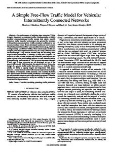
FIGURE CAPTIONS Fig. 1: Time evolution of the partial distribution functions f1 (broken lines) and f2 (solid lines) using Eqs. 24 for Maxwell interaction with parameters T = 2s, a1 = 0.4m/s2 and a2 = −0.2m/s2 . The initial conditions at t = 0 are normal distributions with mean V = 28m/s and variance 0.1m2 /s2 . Fig. 2: Standardized velocity distributions in stochastic equilibrium based on Eq. 26. The brocken line describes the Maxwell type interaction rate, Eq. 31, where the solid line is the relative velocity type interaction rate, Eq. 29. Fig. 3: Equilibrium velocity distributions for different car density values K described in subsection 4.3 with a0 = 0.05m/s2 (solid line) and a0 = 0.2m/s2 (broken line). The following fixed parameter values are used: T = 2.5s, α =1.8s, hmin = 6.5m. Fig. 4: The car density K dependence of the mean velocity V for two different threshold slopes as described in subsection 4.3. The following fixed parameter values are used: T = 2.5s, a0 =0.2m/s2 , hmin = 6.5m. Fig. 5: The car density K dependence of the velocity scattering σv for two different threshold slopes as described in subsection 4.3. The following fixed parameter values are used: T = 2.5s, a0 =0.2m/s2 , hmin = 6.5m. Fig. 6: The car density K dependence of the traffic density K · V for two different threshold slopes as described in subsection 4.3. The following fixed parameter values are used: T = 2.5s, a0 =0.2m/s2 , hmin = 6.5m.
21
Figure 1:
22
0 17
0.3
f1 ,f 2
0.6
21
t=8s t=16s
t=4s
t=2s
t=0.2s
v(m/s)
t=20s
25
Figure 2:
23
0
0.2
0.4
~ feq
−4
−2
0
2
v−V σv
4
Figure 3:
24
0
0.1
0.2
0.3
0.4
^ feq(v)
0
10
K=0.05/m
20
K=0.025/m
30
K=0.014/m
v [m/s] 40
K=0.01/m
Figure 4:
25
0
10
20
30
40
V[m/s]
0
0.02
α=1.8s
α=1.2s
0.04
K[1/m]
0.06
Figure 5:
26
V
0
1
2
3
4
0
σ [m/s]
0.02
α=1.8s
0.04
α=1.2s
K[1/m]
0.06
Figure 6:
27
0
0.1
0.2
0.3
0.4
0.5
K .V[1/s]
0
0.04
α=1.8
α=1.2
0.08
K[1/m]
0.12