NUMERICAL SIMULATION OF BREAKING WAVES USING THE VOLUME OF FLUID METHOD Deborah Greaves School of Engineering, University of Plymouth, Drakes Circus, Plymouth, PL4 8AA U.K. e-mail:
[email protected] Introduction In certain cases of extreme wave loading it is important that the numerical simulation model should include both viscous effects and wave breaking. This usually means solving the Navier Stokes or RANS equations together with a two-fluid interface capturing approach, such as level set or volume of fluid (VoF), in which the fluid dynamics equations are solved both in the air and water. Recent advances in development of high resolution advection schemes for the interface mean that some of the previous disadvantages of VoF methods, such as interface smearing, have been overcome (see e.g.Ubbink, 1997). In this work, the development of a numerical wave tank for investigation of breaking waves is presented. A finite volume discretisation for DNS simulation of the Navier-Stokes equations by pressure-based iteration is used together with the volume of fluid method. The calculation is carried out both in the air and water and the free surface between them captured using a high resolution technique. Two alternative approaches to simulation of breaking waves are discussed. In both cases, a periodic domain is used and the simulation is started from the initial condition determined by analytical theory for a water wave. In the first case the numerical wave tank is initialized using a Stokes third order approximation with wave steepness greater than the breaking threshold. The second approach is to allow two shallow waves to interact and combine to form a steep wave that may break.
Steep Wave in a periodic domain In this first example, a steep gravity water wave is simulated in a domain with periodic boundary conditions. The fluid properties and initial conditions are the same as those used by Chen et al. (1999), Iafrati (2006) and Greaves (2007) and this study extends the preliminary results presented there. The width of the domain is one wavelength, b = λ, the water depth is h = b/2 and the initial condition for the wave elevation, η is 1 2
η ( x ,0 ) = acos( kx ) + a 2 kcos( 2kx )
(1)
3 + a 3k 2 cos( 3kx ) 8
where k = 2π / λ , a is the wave amplitude and the initial wave slope ε = ak . The initial velocity field in the water is u( x , y ,0 ) =
akg ky e cos( kx ) and
v( x , y ,0 ) =
akg ky e sin( kx ) ,
(2a)
ω
(2b)
ω
where ω = gk ( 1− k 2 a 2 ) and the air is initially at rest. The acceleration due to gravity, g = 9.81m/s2 and the liquid Reynolds number is given by Re = g 1 / 2 λ3 / 2 / υ l . The limit for breaking is given by Longuet-Higgins (1985) to be approximately ak = 0.443. Each of the simulations in this section are calculated on a regular 256 x 256 grid. First a non-breaking case, ak = 0.2, is calculated. The ratio of density in air and water, ρ a ρ l = 0.01, the ratio of dynamic viscosities, µ a µ l = 0.4 and the liquid Reynolds number, Re = 3132. The time series of free surface profiles is given in Figure 1
(
)
and shows the smooth repeating form of the wave. The profiles are plotted with the mean water level at their simulation time in seconds in the vertical direction and a second wavelength is plotted on the right hand side of each to clarify the figure.
3
2.5
2
1.5
2.5 1
2 0.5
1.5
0 −0.5
1
1
1.5
3
2.5
0
0
0.5
1
1.5
Figure 1 Time sequence of wave profiles, ak = 0.2, Re = 3132, ρ a ρ l = 0.01, µ a µ l = 0.4.
Next, a series of steep waves with ak = 0.55, beyond the breaking limit, is calculated and results presented in Figures 2 - 5. In Figure 2, the Reynolds number is Re = 3132, ρ a ρ l = 0.01, µ a µ l = 0.4; in Figure 3, the Reynolds number is increased to Re = 10,000; in Figure 4, the density ratio is reduced to ρ a ρ l = 0.001; and in Figure 5, the viscosity ratio is reduced to µ a µ l = 0.017. 3
2
1.5
1
0.5
0 −0.5
0
0.5
1
1.5
Figure 4 Time sequence of wave profiles, ak = 0.55, Re = 104, ρ a ρ l = 0.001, µ a µ l = 0.4. 3
2.5
2.5
2
2
1.5
1.5
1
1
0.5
0.5
0
0 −0.5
0.5
Figure 3 Time sequence of wave profiles, ak = 0.55, Re = 104, ρ a ρ l = 0.01, µ a µ l = 0.4.
0.5
−0.5
0
0
0.5
1
1.5
Figure 2 Time sequence of wave profiles, ak = 0.55, Re = 3132, ρ a ρ l = 0.01, µ a µ l = 0.4.
−0.5
0
0.5
1
1.5
Figure 5 Time sequence of wave profiles, ak = 0.55, Re = 104, ρ a ρ l = 0.001, µ a µ l = 0.017.
Features of the wave, such as the steepening of the wave, development of a plunging jet and successive splash ups are similar to those observed by Iafrati (2006) and Rapp and Melville (1990), as discussed by Greaves (2007) previously at this Workshop. Here, we investigate how in each of the successive simulations, the physical properties are closer to those of air and water and the predicted breaking becomes more violent. As the Reynolds number is increased, wave breaking is initiated earlier and the overturning jet is sharper. This effect is increased when the density ratio is reduced in line with the physical properties of air and water in Figure 4. In Figure 5, the viscosity of the air is reduced and this further sharpens the jet as the crest overturns and increases the predicted spray associated with the breaking event. Reducing the liquid viscosity to that of water would lead to a much higher Reynolds number, O(106) and turbulence would need to be taken into account in the numerical model.
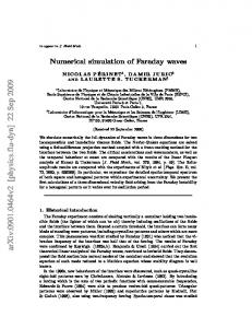
Results of simulations with increasing values of wave steepness, k1a1 = k2a2 are presented to illustrate the progression to wave breaking. In Figures 6 – 9, wave profiles are plotted for k1a1 = k2a2 = 0.17, 0.18, 0.19 and 0.22. Physical properties are set up such that Re = 104, ρ a ρ l = 0.001, µ a µ l = 0.017 and g = 9.81 m/s. As before, in Figures 1 – 5, a second wavelength of the longer wave is plotted alongside the first for clarity. 3
2.5
2
1.5
1
0.5
0 −0.5
0
0.5
1
1.5
Figure 6 Interacting waves, k1a1 = k2a2 = 0.17.
Interaction of two linear waves
3
Another approach to investigating wave breaking is to allow two regular waves to interact, as used by Rainey (2007) to demonstrate particle escape. Here, waves are defined in a periodic domain, as above, but the waves are given initial velocity and free surface profiles from linear theory. The two waves have 2:1 length ratio, and their parameters are wavenumber, k1 =6.28 and k2 = 12.57, frequency, ω1 and ω 2 (assuming deep water, ω = kg ) and amplitude a1 and a2. The initial conditions for surface elevation and particle velocity are given by linear theory as η ( x ,0 ) = a1cos( k1 x ) + a 2 cos( k 2 x ) u( x , y ,0 ) = ω1a1e k1 y cos( k1 x )
(3) (4a)
+ ω 2 a 2 e k 2 y cos( k 2 x ) v( x , y ,0 ) = ω1a1e k1 y sin( k1 x ) + ω 2 a 2 e k2 y sin( k 2 x ) .
(4b)
2.5
2
1.5
1
0.5
0 −0.5
0
0.5
1
1.5
Figure 7 Interacting waves, k1a1 = k2a2 = 0.18.
Although the steepness of each wave is considerably less than the breaking limit, the two waves interact with one another and may break. Similar calculations were carried out by Rainey (2007) using a fully-nonlinear potential flow program based on the boundary integral method, which is able to predict the wave profile up to breaking, but breaks down
after the crest jet is formed. Rainey (2007) investigated the threshold for wave breaking and particle escape as an indicator for wave breaking. When computed with first order initial conditions, these limits were ka = 0.19 and 0.17 respectively and when initiated with second order wave profile and velocity potential, the thresholds were predicted to be ka = 0.18 for wave breaking and 0.21 for particle escape. 3
2.5
2
1.5
1
method is shown to be a valuable tool for investigating wave breaking and nonlinear wave interaction. The aim is to extend the method to simulate extreme wave loading on and overtopping of coastal, offshore and floating structures. In order to do this, the wave must be generated by defining a wavemaker boundary condition at the inlet on the left hand side of the tank and to have the initial condition of stationary still water. The wavemaker boundary condition may be applied either as a moving piston or as imposed velocity and wave elevation at the wavemaker, using either linear of higher order wave theory. This step introduces difficulties, such as problems of reflection from the right hand wall and instability generated by the large difference in density between the two fluids.
0.5
References 0 −0.5
0
0.5
1
1.5
Figure 8 Interacting waves, k1a1 = k2a2 = 0.19. 3
2.5
2
1.5
1
0.5
0 −0.5
0
0.5
1
1.5
Figure 9 Interacting waves, k1a1 = k2a2 = 0.22.
In this work, wave breaking is evident for ka = 0.17 and increases in violence as the wave steepness is increased. The mode of breaking can be seen to progress through Figures 6 – 9 from spilling towards plunging (Bonmarin, 1989). Conclusions In the preliminary results presented here, the
Iafrati, A. 2006 Effect of the wave breaking mechanism on the momentum transfer, 21st International Workshop on water wave and floating bodies, Loughborough, 2-5 April 2006. Bonmarin, P. 1989 Geometric properties of deep water breaking waves, Journal of Fluid Mechanics, 209, 405 – 433. Rapp, R.J. and Melville, W.K. 1990 Laboratory measurements of deep-water breaking waves, Phil. Trans. Royal Society London, Series A, 331:1622, pp. 735 – 800. Ubbink, O. 1997 Numerical prediction of two fluid systems with sharp interfaces, PhD Thesis, Imperial College of Science, Technology and Medicine, London. Longuet-Higgins, M.S. 1985 The asymptotic behaviour of the coefficients in Stokes’s series for surface gravity waves, IMA Journal of Applied Mathematics, 34, 269 – 277. Greaves D.M. 2007 Numerical simulation of breaking waves and wave loading on a submerged cylinder 22nd International Workshop on water wave and floating bodies, Plitvice, Croatia, 15 - 18 April 2007. Rainey R.C.T. 2007 Weak or strong nonlinearity: the vital issue, Journal of Engineering Mathematics, 58, 229 – 249.