Numerical Simulation of Sand Erosion Phenomena in ... - CiteSeerX

Proceedings of the 8th International Symposium on Experimental and Computational Aerothermodynamics of Internal Flows Lyon, July 2007

ISAIF8-0093

Numerical Simulation of Sand Erosion Phenomena in Rotor/Stator Interaction of Compressor Masaya Suzuki, Kazuaki Inaba and Makoto Yamamoto Department of Mechanical Engineering, Tokyo University of Science, 1-14-6, Kudankita, Chiyoda-ku, Tokyo, 102-0073, Japan

Sand erosion is a phenomenon where solid particles impinging to a wall cause serious mechanical damages to the wall surface. This phenomenon is a typical gas-particle two-phase turbulent flow and a multi-physics problem where the flow field, particle trajectory and wall deformation interact with among others. On the other hand, aircraft engines operating in a particulate environment are subjected to the performance and lifetime deterioration due to sand erosion. Especially, the compressor of the aircraft engines is severely damaged. The flow fields of the compressor have strongly three dimensional and unsteady natures. In order to estimate the deterioration due to sand erosion, the sand erosion simulation for a compressor is required under the consideration of the rotor-stator interaction. In the present study, we apply our three dimensional sand erosion prediction code to a single stage axial flow compressor. We numerically investigate the change of the flow field, the particle trajectories, and the eroded wall shape in the compressor, to clarify the effects of sand erosion in the compressor.

Keywords: sand erosion, axial compressor, rotor/stator interaction, computational fluid dynamics

Introduction The basic researches for sand erosion phenomena started centering on Germany in 1930's. Finnie attempted the theoretical analysis on sand erosion, based on the Hertz’s contact theory [1]. However, Finnie's model cannot exactly predict the weight loss in high angle impact. Then, Bitter suggested the mechanism of sand erosion which consists of deformation wear and cutting wear [2, 3]. Bitter's model gives the sufficient prediction in any impinging angle for both of the ductile and brittle materials, but this model is too complex to easily apply for industrial machines. Therefore, Neilson and Gilchrist modified the model to apply for practical calculation based on Bitter's concept [4, 5].

On the other hand, aircraft engines operating in a particulate environment are subjected to the performance and lifetime deterioration due to sand erosion. Especially, the compressor of the aircraft engines is severely damaged. Balan and Tabakoff [6] performed the experimental study of sand erosion phenomena on a single stage axial flow compressor, and found severe erosion on the leading edge and pressure side of rotor blades, with the increased surface roughness. In recent years, sand erosion phenomenon has been simulated numerically to protect industrial machines from the mechanical damage. In these simulations, however, the change of the flow field and the relating particle trajectory during the erosion process were not taken into account. This treatment is physically unrealistic. Hence,

Masaya Suzuki: Graduate Student http://www.lmfa.ec-lyon.fr/ISAIF8/

2

Proceedings of the 8th International Symposium on Experimental and Computational Aerothermodynamics of Internal Flows

we have developed the numerical procedure for sand erosion phenomenon, including the temporal change of the flow field and the wall shape [7]. This numerical code was successfully applied to a 90-degree bend [8], particle separator [9], turbine stator blade [10], and so on. The flow fields in these studies are steady, but the flow field in a compressor has strongly unsteady characters by rotaNomenclature CD drag coefficient specific heat at constant pressure Cp D diameter e total energy F drag force k turbulent kinetic energy K maximum particle velocity at which the collision still is purely elastic eroded cavity length lc M mass n material parameter decides α0 p static pressure Pk production rate of k Pr Prandtl number Re Reynolds number S strain rate t time T static temperature U velocity V impinging velocity W eroded weight x Cartesian coordinate

Numerical Procedures The computational procedures for the prediction of sand erosion phenomenon are as follows: (1) Calculate the turbulent flow field (2) Calculate the particle trajectories (3) Judge the collisions against a wall (4) Estimate the amount of erosion (5) Change the wall shape (6) Return to (1), if the wall shape is changed. These procedures are repeated iteratively, until the computational time reaches the prescribed terminal time. Normally, since the sand erosion phenomenon needs a long period, and the time scale is much longer than that of the flow field, the change of flow field could be regarded as a quasi-steady state. Therefore, steady state flow distributions are thought to be valid for each eroded geometry and at every instance. This means that in the present study sand erosion phenomenon is mimicked as series of quasi-steady states. However, in a compressor stage, rotor rotation brings about strong unsteadiness

tion of the rotor blades. Therefore, it is essential to consider the unsteadiness. In the present study, we apply our three dimensional sand erosion prediction code to a single stage axial flow compressor. We numerically investigate the temporal change of the flow field, the particle trajectories, and the eroded wall shape in the compressor, to clarify the effects of sand erosion.

Greek letters impinging angle attack angle at which the tangential component of the reflection velocity comes to be zero Kronecker delta δ turbulent dissipation rate ε φ energy needed to remove unit weight from wall by cutting wear viscosity coefficient µ kinetic viscosity coefficient ν density ρ energy needed to remove unit weight from wall ψ by deformation wear vorticity Ω

α α0

Subscripts C cutting D deformation f fluid p particle t turbulent T total which must be considered. Hence, we store the data of temporal flow field corresponding to a rotor-stator blade position, and use it to calculate particle trajectories. Gas-phase Numerical predictions have been carried out with a finite difference technique. The gas-phase is considered to be a continuum phase, while the particle-phase is a dispersed one. The particle-phase that is assumed to be of low concentration has no influence on the gas-phase (i.e. one-way coupling). The gas-phase flow is assumed to be three-dimensional, compressible and turbulent. It is calculated by the Eulerian approach, based on the Favre-averaged Navier-Stokes equations (i.e. RANS approach). The governing equations with the standard k-ε turbulence model (Launder-Spalding, 1974) are expressed as follows, (Continuity equation): ∂ρ ∂ (ρU j ) = 0 + (1) ∂t ∂xi

Masaya Suzuki et al.

Numerical Simulation of Sand Erosion Phenomena in Rotor/Stator Interaction of Compressor

(Favre-Averaged Navier-Stokes equation): ∂ (ρU i ) + ∂ (ρU iU j + pδ ij ) ∂t ∂x j =

∂  2  (µ + µ t )S ij − ρkδ ij  ∂x j  3 

(2)

(Energy equation): ∂ (ρe ) + ∂ {(ρe + p )U j } ∂t ∂x j

=

(3)   µ µ t  ∂T  2    ( ) + − + + S k U C µ µ ρ δ   t ij ij  i p  3   Pr Prt  ∂x j   ∂U i ∂U j 2 ∂U k ∂U i ∂U j (4) δ ij , Ω ij = S ij = + − − ∂x j ∂xi 3 ∂x k ∂x j ∂xi

∂ ∂x j

(k-ε model):  ∂ (ρk ) + ∂ (ρkU j ) = ∂  µ + µ t ∂t ∂x j ∂x j  σk + ρ (Pk − ε )

 ∂k     ∂x j 

(5)

 ∂ (ρε ) + ∂ (ρεU j ) = ∂  µ + µ t ∂t ∂x j ∂x j  σε

 ∂ε     ∂x j 

(6)

+ρ

ε k

(C

ε1

Pk − Cε 2 ε )

2   ∂U i Pk = υ t S ij − kδ ij  3   ∂x j

υt = Cµ

k2

ε

the following assumptions are made for reducing the computational load: z Particle is spherical and non-rotating. z Particle-particle collision is neglected. z The particle-phase has no influence on the gas-phase. z The force acting on a particle is only a drag. Under these assumptions, the equation of the particle motion is described using a relative velocity of the gas-phase to the particle. dU pi = F (U fi − U pi )U fi − U pi (11) dt 3C D ρ f (12) F= 4ρ p D p where Up, ρp and Dp are density, velocity and diameter of a particle. F denotes drag force, and the drag coefficient CD is defined by calculating the relative particle Reynolds number based on the relative velocity between the gas-phase and the particle as follows,  24 (1 + 0.15 Re 0p.687 ) (Re p < 1000) (13)  C D =  Re p 0.4 (Re p > 1000) 

Re p =

(7) (8)

where C µ = 0.09 , σ k = 1.0 , σ ε = 1.3 , Cε 1 = 1.44 , Cε 2 = 1.92 . ρ, U, p, T and e denote the averaged component of density, velocity, pressure, temperature and total energy of fluid. k and ε are turbulent kinetic energy and its dissipation rate. Since standard k-ε model excessively predict turbulence energy production for irrotational strain, Kato-Launder’s modification (1993) was adopted. Then, Pk was modified as follows, ~ Ω ~ 2 ∂U k  Pk = ~ υ t S 2 − k (9) 3 ∂x k  S  1 (S ij S ij + S ii S jj ) , Ω~ = 1 Ω ij Ω ij (10) 2 2 The governing equations were discreted using Yee-Harten’s second-order upwind TVD scheme (1987) for the inviscid terms, second-order central difference scheme for the viscous ones, and 4-stage Runge-Kutta method for the time integration. ~ S =

Particle-phase

The particle-phase is treated by the Lagrangian approach, in which particles are tracked in time along their trajectories through the flow field. In the present study,

3

D p U fi − U pi

υ

(14)

where ν is kinetic viscosity of gas-phase. Finally the particle trajectory is calculated by integrating the following equation in time with the leap flog method. dx pi = U pi (15) dt Erosion estimation

It is well known that Finnie [1] had an important role to the early analysis of sand erosion. And Bitter [2, 3] suggested that sand erosion damage due to particle impacts can be considered to be separate mechanisms, that is, deformation wear due to the velocity normal to the surface and cutting wear due to the tangential velocity. The total volume loss WT is the sum of the volume losses due to deformation wear WD and cutting wear WC. WT = WD + WC (16) However, since Bitter’s theoretical work is exhaustive and extremely intricate, it is too difficult to employ his model in practical applications. Therefore, the simpler relations based on the Bitter’s model were proposed by Neilson and Gilchrist [4, 5], in which the weight losses WD and WC can be rewritten as, 1 2 M (V sin α − K ) 2 (17) W = D

ψ

4

Proceedings of the 8th International Symposium on Experimental and Computational Aerothermodynamics of Internal Flows

1 2 2  2 MV cos α sin nα   φ WC =  1  MV 2 cos 2 α 2   φ

α0 =

(α < α ) 0

(18)

(α ≥ α ) 0

π

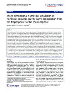
(19) 2n where M is total mass of particles, α and V are the attack angle and the impinging velocity of a particle. K is the threshold value of the velocity component normal to the surface, below which no deformation wear takes place. α0 is the attack angle at which the tangential component of the reflection velocity comes to be zero (see Fig. 1). n is constant and depends on a surface material. ψ and φ represent the energy needed to remove the unit weight of material from the wall by deformation and cutting wear, respectively. Using the experiment by Neilson and Gilchrist [4, 5], these parameters were confirmed to predict sand erosion. In the present study, the above-described Neilson-Gilchrist erosion model is employed because of the simplicity. However, the geometrical information of eroded surface, that is, the length and depth of the cavity removed, cannot be obtained from the Neilson-Gilchrist erosion model, because Eq. (17) and (18) describes only the weight loss of the surface material. Thus, the eroded surface geometry damaged by one particle, which consists of the deformation wear (the volumes of A) and the cutting wear (that of B), is assumed as shown in Fig. 2. Considering the concept of Neilson-Gilchrist model, this assumption is reasonable, and the modeled cavity is similar to the experimental observation by Bitter [2, 3].

Fig. 1

The weight losses due to deformation wear WD and cutting wear WC can be geometrically expressed as follows, using the symbols in Fig. 2,  Dp WD = ρπ   2

  

3

 cos 3 θ p + 2   − cos θ p   3  

(20)

2

 Dp   1   θ p − sin 2θ p  (21) WC = ρl c  2 2     The following procedure is adopted to calculate the erosion length lc. (1) WD and WC are obtained by the Neilson-Gilchrist erosion model. (2) Substituting WD into Eq. (20), θp is calculated. (3) Substituting WC and θp into Eq. (21), the erosion length lc is estimated. In order to reproduce a sand erosion phenomenon in a 3-D computational field, we suggest the “erosion line” approach. In this approach, an erosion cavity is approximated by a line with the length lc, taking into account that the width of erosion cavity is sufficiently small, compared with the three-dimensional grid spacing on a wall surface. Figure 3 explains our definition for an erosion line. Erosion line approach is summarised below. (1) Erosion line lc is laid on the surface in the computational domain (see Fig. 3). (2) The length occupied by each grid cell is calculated. (3) Partial weight loss is assigned in each block in proportion to the partial length lc(i). (4) If the partial weight loss on a block exceeds the critical value, the block in the wall drops out. The dropped cell region is newly treated as the flow field instead of a solid wall. This change of the surface geometry indicates the evolution of a sand erosion phenomenon. It should be noted that blocks in a wall and the weight of each block are set prior to a calculation.

Schematic of particle impact against wall

Fig. 3

Fig. 2

Modeled erosion cavity

Erosion line approach

The computational grid consists of two regions, that is, in a flow field and within a solid wall. The block height in the wall is uniform and is same as the minimum one in the flow field.

Masaya Suzuki et al.

Numerical Simulation of Sand Erosion Phenomena in Rotor/Stator Interaction of Compressor

using erosion model. In the rebound at end walls, particle impingement is treated as perfect elastic impingement.

Computational Conditions The computations were carried out for the single stage axial flow compressor measured by Balan and Tabakoff [6]. The design specifications of the compressor are listed in Table 1. The compressor blade is NACA65 (10)-10 airfoils [11]. The compressor does not have any guide vanes, and the rotor diameter is constant for the axial direction. Figure 4 shows the schematic of the target compressor stage. The test conditions are listed in Table 2. In the present study for the simplicity, it was assumed that the tip clearance was 0 and that the tip and hub walls rotated with rotor blades. Table 1

Table 2

Fig. 4

Schematic of axial flow compressor stage

Design specifications

Airfoil Chord length Aspect ratio Solidity Tip diameter Rotating speed Pressure ratio Mass flow rate

NACA65 (10)-10 50.8 [mm] 0.75 2 300 [mm] 9000 [rpm] 1.1 3.67 [kg/s]

(a) 2D section of rotor and stator

Operation conditions

Rotating speed Inlet total pressure Inlet total temperature Mass flow rate

5

5000 [rpm] 1.013×105 [Pa] 288.15 [K] 1.360 - 2.000 [kg/s]

Figure 5 plots the computational grid used in the present simulation. The grid numbers in the flow fields were 900,000, and those within the blade walls were 300,000. Thus, the total grid number was 1,200,000. The region around the rotor blade was computed in relative coordinate system, on the other hand, the region around the stator blade was treated in absolute coordinate system. The boundary conditions were imposed as follows. At the inlet boundary, flow angle, total pressure and total temperature were fixed. At the exit, static pressure was specified. On the blade surfaces, non-slip and adiabatic conditions were imposed. On the end walls, slip and adiabatic conditions were used. The turbulent quantities were decided by the wall function. At the side boundaries, periodic condition was used (computational domain was 1 pitch). The materials of solid particles and the wall were assumed to be alumina and aluminum, respectively. The particle diameter was 165 µm. The total mass of the inlet particles is 25 kg. In the particle trajectory calculation, the rebound velocity at the blade surface is estimated by

(b) Rotor main grid

(c) Rotor sub grid Fig. 5

Computational grids

6

Proceedings of the 8th International Symposium on Experimental and Computational Aerothermodynamics of Internal Flows

Results and Discussion Change of flow field

Figures 6 and 7 depict Mach number and static pressure contours at midspan of clear blades. In the case with mass flow rate of 1.75 [kg/s], inlet Mach number is 0.14 and the maximum Mach number is 0.28. Consequently, these are subsonic cascade. Furthermore, inlet and outlet static pressure are respectively 9.985×104 and 1.025×105 [Pa]. As not shown here, but separation vortexes are confirmed on the rotor and stator blade root. Static temperature and turbulent kinetic energy contours at midspan of clear blades are shown in Figs. 8 and 9. It is clear that the wake of rotor blade is chopped by the stator blade. The development of the boundary layer is promoted around the region where the wake of rotor blade impinges on the stator pressure side. The fluid which has high turbulent kinetic energy passes the stator blades passage periodically. It is confirmed that representative rotor/stator interaction is reproduced in our computation. Figure 10 illustrates the comparison of the vorticity contours on rotor blade pressure side before and after erosion. Since the surface of the pressure side is severely rough, as shown later, the velocity disturbances generated

Fig. 6

Fig. 8

Mach number contour at midspan

Static temperature contour at midspan

on the pressure side is remarkable. Thus, the irregularity of vorticity becomes high after erosion. Static pressure contours at the leading edge of the clear and eroded rotor blade surface are exhibited in Fig. 11. Similarly to the vorticity, static pressure becomes nonuniform. Static pressure on the pressure surface is smaller than that of the uneroded blades, additionally. This is because the boundary layer thickness becomes thick due to the growth of surface roughness, and then the freestream velocity between the blades increases. Eroded surface

Figure 12 shows the change of the blade surface due to sand erosion. Severe erosion occurs around the leading edge and on the pressure surface. The pressure side of the rotor blade suffers from severe damage over wide region especially. The tip is severely eroded rather than the hub. On the rotor blade suction surface, a little wear is confirmed around the leading edge. And no erosion occurs on the downstream region from the mid chord. Moreover, the suction side of the stator blade keeps a clear surface. These results would be affected by the interactions among impinging velocity, angle and frequency. The reasons why the eroded surface is formed will be discussed in the following sub sections.

Fig. 7

Fig. 9

Static pressure contour at midspan

Turbulent kinetic energy contour at midspan

Masaya Suzuki et al.

Numerical Simulation of Sand Erosion Phenomena in Rotor/Stator Interaction of Compressor Tip

7

Tip

L.E.

L.E.

T.E.

T.E.

Hub

Hub

(b) After erosion

(a) Before erosion Fig. 10

Vorticity contour of the rotor blade pressure surface

Tip

Tip

S.S.

S.S.

P.S.

P.S.

Hub

Hub

(b) After erosion (a) Before erosion Fig. 11 Static pressure contour of the rotor blade leading edge Tip

L.E.

Hub

T.E.

T.E.

(a) Rotor pressure surface

Tip

L.E.

Tip

T.E.

Hub

(b) Rotor suction surface Fig. 12

Hub

L.E.

L.E.

(c) Stator pressure surface Eroded surface

Tip

T.E.

Hub

(d) Stator suction surface

8

Proceedings of the 8th International Symposium on Experimental and Computational Aerothermodynamics of Internal Flows

(a) Bird eye view

(c) Top view

(b) Side view Fig. 13

Particle trajectory

Particle trajectories

The typical particle trajectories are plotted in Fig. 13. The particle trajectories around the rotor are shown in relative coordinate system and those around the stator are exhibited in absolute coordinate system. The colors correspond to the particle speed (black: high speed, white: low speed) in each coordinate system. Obviously, the particles reflect around the rotor blade leading edge or pressure side, and most of the kinetic energy is consumed by the erosion of the first impact. The particle has less kinetic energy at the second impact to the suction surface, and thus the mechanical damage on the suction surface is not so severe. When the particle velocity becomes small by the particle-wall collision in the rotor blades passage, Coriolis and centrifugal forces are dominant, and the particle rapidly moves towards the tip (Fig. 13(b)). Then, the particle goes through the rotor passage with the repeated impacts to the pressure and suction sides and end wall (Fig. 13(c)). On the other hand, the particle inflowing into the stator has large velocity due to the rebound on the rotor blade and the rotor rotation. Therefore, most of the particle impact to the leading edge of the stator blade at high speed. Note that the particle dose not impinge on the downstream region from the mid chord of the pressure side. It is caused from the fact that the particle has high circumferential velocity. As same as in the rotor blade passage, the particle consumes its kinetic energy at the first impact, and flows towards the downstream with repeated impacts to the pressure and suction sides. Impact properties

Figure 14 shows the impact frequency distribution. The impingement to blade surface concentrates around the trailing edge of the rotor blade and the leading edge of the stator blade. And the high impact frequency is

found on the pressure surface of the rotor blade and the mid chord region of stator blade suction side. The impact frequency of the tip is much higher than that of the hub. This is caused by the high concentration of particles in the rotor passage due to centrifugal force (Fig. 13(b)). We defined average eroded weight, dividing the total eroded weight by the total impingement number at every grid cell on the blade surface. Figure 15 exhibits the average eroded weight distributions. In the rotor, most of the pressure surface suffers from severe damage due to one particle impingement. Additionally, the leading edges of both rotor and stator blade are exposed to high damage impact. The first impact velocity is proportion to the radial position from the axis because of the rotation, the damage of the tip is severer than that of the hub. Note that the low damage region exists at the tip of the rotor blade. Nevertheless, this does not mean the tip erosion is not severe. This results from that the rebounded particle collides against the rotor tip secondarily with low velocity and high angle. Figure 16 indicates average impact velocity, and Fig. 17 illustrates impact angle. These are averaged similarly to average eroded weight. The particle impinges to the pressure side of the rotor blade with high velocity. Moreover, the average impact velocity is high at the leading edge and tip. This result matches with the behavior of average eroded weight. The high angle collision occurs frequently on the suction surface of both rotor and stator blade. In addition, the high angle impingement is confirmed at the trailing edge of the rotor blade pressure side. This leads no pronounced erosion on the region. Because weight loss of ductile material at high angle impingement is smaller than that at low angle.

Masaya Suzuki et al.

Numerical Simulation of Sand Erosion Phenomena in Rotor/Stator Interaction of Compressor

Tip

L.E.

Hub

T.E.

T.E.

(a) Rotor pressure surface

Tip

L.E.

Hub

T.E.

(b) Rotor suction surface Fig. 14

Tip

L.E.

Hub

T.E.

T.E.

(a) Rotor pressure surface

Tip

L.E.

Hub

T.E.

(a) Rotor pressure surface

Tip

Tip

L.E.

Hub

(a) Rotor pressure surface

Tip

Tip

T.E.

Hub

(d) Stator suction surface

Hub

L.E.

L.E.

(c) Stator pressure surface

Tip

T.E.

Hub

(d) Stator suction surface

Average eroded weight L.E.

Tip

T.E.

Hub

L.E.

L.E.

(c) Stator pressure surface

Tip

T.E.

Hub

(d) Stator suction surface

Average Impact Velocity L.E.

Tip

T.E.

Hub

(b) Rotor suction surface Fig. 17

Tip

T.E.

Hub

T.E.

T.E.

L.E.

(b) Rotor suction surface Fig. 16

L.E.

(c) Stator pressure surface

Hub

T.E.

Hub

L.E.

Impact frequency

(b) Rotor suction surface Fig. 15

Tip

Tip

9

Hub

L.E.

L.E.

(c) Stator pressure surface

Average Impact Angle

Tip

T.E.

Hub

(d) Stator suction surface

10

Proceedings of the 8th International Symposium on Experimental and Computational Aerothermodynamics of Internal Flows

Concluding Remarks We carried out the numerical simulations for the sand erosion phenomena in the rotor/stator interaction of the single stage axial flow compressor. Through the present study, we obtained the following insights. (1) Since the surface of the pressure side is severely rough, the nonuniformity of the vorticity and static pressure becomes high. This changes the static pressure distribution on the blade. (2) Severe sand erosion occurs on the pressure surface and leading edge of the blades. (3) Tip is deteriorated by sand erosion rather than hub due to high impact velocity. (4) In both of the rotor and stator blades, particle-wall collisions repeatedly occur, but the first impacts are dominant and the most important to erosion.

Acknowledgement This paper owes much to the help of I. Mizuta and D. Kato in Ishikawajima-Harima Heavy Industries Co., Ltd. In addition, this research was partially supported by the Ministry of Education, Science, Sports and Culture, Grant-in-Aid for Scientific Research (C) 16560158.

References [1] Finnie, I.: Erosion of surfaces by solid particles, Wear, vol.3, pp.87-103, (1960).

[2] Bitter, J. G. A.: A study of erosion phenomena part I, Wear, vol.6, pp.5-21, (1963). [3] Bitter, J. G. A.: A study of erosion phenomena part II, Wear, vol.6, pp. 169-190, (1963). [4] Neilson, J. H. and Gilchrist, A.: Erosion by a stream of solid particle, Wear, vol.11, pp.111-122, (1968). [5] Neilson, J. H. and Gilchrist, A.: An experimental investigation into aspects of erosion in rocket motor nozzles, Wear, vol.11, pp.123-143, (1968). [6] Balan, C. and Tabakoff, W.: Axial Flow Compressor Performance Deterioration, AIAA-84-1208, (1984). [7] Kuki, J., Toda, K., Yamamoto, M.: Development of Numerical Code to Predict Three-Dimensional Sand Erosion Phenomena, FEDSM2003-45017, Proc. ASME FEDSM'03 4TH ASME_JSME Joint Fluids Engineering Conference, Honolulu, (2003). [8] Miyama, T., Nakayama, T., Kitamura, O. and Yamamoto, M.: Numerical Prediction of Sand Erosion along Curved Passages, Proc. Third World Conference in Applied Computational Fluid Dynamics, 27, pp.53-60, (1996). [9] Kuki, J., Toda, K., Yamamoto, M.: Numerical Simulation of Sand Erosion Phenomena in a Particle Separator, Key Engineering Materials, 243-244, pp. 565-570, (2003). [10] Suzuki, M., Toda, K. and Yamamoto, M., Numerical Simulation of Sand Erosion Phenomena on Turbine Blade Surface, Proc. WCCM VI in conjunction with APCOM'04, Beijing, (2004). [11] Emery, J. C., Herring, L. J., Erwin, J. R. and Felix, A. R.: Systematic Two-Dimensional Cascade Tests of NACA 65-Series Compressor Blades at Low Speeds, NACA Report 1368.