Keywords Rock fracture ภContact mechanics ภElastic contact ภ..... 3 Contact Mechanics ...... Earth Planet Sci Lett 281:81â87. https ://doi.org/10.1016/j.
Rock Mechanics and Rock Engineering https://doi.org/10.1007/s00603-018-1498-x
ORIGINAL PAPER
Numerical Simulations and Validation of Contact Mechanics in a Granodiorite Fracture Tobias Kling1 · Daniel Vogler2,3 · Lars Pastewka4,5 · Florian Amann6 · Philipp Blum1 Received: 13 October 2017 / Accepted: 3 May 2018 © Springer-Verlag GmbH Austria, part of Springer Nature 2018
Abstract Numerous rock engineering applications require a reliable estimation of fracture permeabilities to predict fluid flow and transport processes. Since measurements of fracture properties at great depth are extremely elaborate, representative fracture geometries typically are obtained from outcrops or core drillings. Thus, physically valid numerical approaches are required to compute the actual fracture geometries under in situ stress conditions. Hence, the objective of this study is the validation of a fast Fourier transform (FFT)-based numerical approach for a circular granodiorite fracture considering stress-dependent normal closure. The numerical approach employs both purely elastic and elastic–plastic contact deformation models, which are based on high-resolution fracture scans and representative mechanical properties, which were measured in laboratory experiments. The numerical approaches are validated by comparing the simulated results with uniaxial laboratory tests. The normal stresses applied in the axial direction of the cylindrical specimen vary between 0.25 and 10 MPa. The simulations indicate the best performance for the elastic–plastic model, which fits well with experimentally derived normal closure data (root-mean-squared error = 9 µm). The validity of the elastic–plastic model is emphasized by a more realistic reproduction of aperture distributions, local stresses and contact areas along the fracture. Although there are differences in simulated closure for the elastic and elastic–plastic models, only slight differences in the resulting aperture distributions are observed. In contrast to alternative interpenetration models or analytical models such as the Barton–Bandis models and the “exponential repulsion model”, the numerical simulations reproduce heterogeneous local closure as well as low-contact areas ( 1 mm are excluded to ease comparison
The elastic material properties of the intact granodiorite are estimated from uniaxial compression tests, which yield a static Young’s modulus E between 10 and 12 GPa (Vogler et al. 2018). Since there are no explicit measurements of the Poisson ratio, a Poisson ratio of 0.3 is assumed in this study, which is similar to the value determined by Keusen et al. (1989) for other Grimsel granodiorite samples. However, it is found in previous contact mechanical studies that deviations from the actual Poisson ratio have only small effects on the simulations (Hyun et al. 2004; Pei et al. 2005). Although the sample-specific E is determined through uniaxial compression tests on the Grimsel granodiorite, values from the
1 0.5
0
5000 4000 3000 2000 1000 0
0
120
Elastic-plastic model (EP)
Elastic model (EL)
Composite surface a0(x,y) Composite surface a0(x,y) Relative hardness H/E* Normale stress n Normale stress n
Boundary Element Method (BEM)
am(x,y) = f(a0(x,y), E* = 1 GPa, n(x,y)) u(x,y)
am(x,y)
a0(x,y)
Initial fracture surface a0(x,y): - Composite surface with ʅ3 contacts: IP1-BB - Composite surface with 1 contact: IP2-BB - Preloaded composite surface: IP3, IP4
n
(x,y)
am(x,y)
Input
Predefined threshold (e.g. closure u): - uBarton-Bandis: IP1-BB, IP2-BB - uexp: IP3, IP4
Predefined uniform closure am(x,y) = a0(x,y) - u
u(x,y) = u
n n(x,y) =H/E*
(x,y)
Interpenetration model (IP)
Ar
a0(x,y)
Method
u Ar
}
n
0.1 0.2 0.3 0.4 0.5 0.6 0.7 0.8 0.9 1.0 Local initial aperture a 0(x,y) [mm]
}
a0(x,y)
(x,y)
am(x,y) = f(a0(x,y), n(x,y), E* = 1 GPa, H/E*) u(x,y)
n n
Boundary Element Method (BEM)
0
}
Fig. 3 Workflow of the adaption process for the fast Fourier transform (FFT)-based elastic (EL) and elastic–plastic (EP) models and the interpenetration models (IP) including the required data input, the schematic contact models and the final data output. Four approaches for the IP models are applied differing by their initial aperture field a0(x,y) and closure data (IP1–IP4). Closure data derived by the Barton– Bandis (BB) model facilitate the choice of a0(x,y) at σn = 0 MPa. Experimental closure data require the potential initial composite fracture surface at σn = 0.25 MPa
60 40 X-direction [mm]
0
6000
Ar
am(x,y)
Renormalization for material properties E* = f(Eexp, vexp)
Local apertures am(x,y) Average aperture am Normal closure u = a0 - am Local closure u(x,y) Contact stresses n(x,y) Real contact area Ar
Local apertures am(x,y) Average aperture am Real contact area Ar
Output
13
T. Kling et al. 12 Granitic rocks (Literature, 115 samples) Grimsel Granodiorite (Literature) Westerley Granite (Literature) Regression: H = 0.14 × E* (R² = 0.68, RMSE = 0.69 GPa) H-range for "very hard" granitic rocks Specimen B (Grimsel Granodiorite)
10
Indentation hardness H [GPa]
literature are collected to define a reasonable range of E for the sensitivity analysis (Table 2). Material properties are also taken for quartz as the theoretical uppermost material boundary (in regard to stiffness) by assuming that the asperities are only in contact along quartz grains representing the dominant rock-forming mineral (30%) besides feldspars (55%) of the granodiorite (Keusen et al. 1989; Wehrens et al. 2017). Furthermore, the extensively investigated Westerly granite and a granodiorite sample from another testing location of the GTS, whose mechanical properties lie in between the experimental and quartz data are taken into consideration. Indentation hardness values, which typically describe the resistance against non-elastic deformation (Brown and Scholz 1986), are obtained from the literature. There are several hardness studies about quartz, which illustrate how relative hardness can vary due to the choice of the indentation hardness H (Table 2). Only for the Westerly granite directly related, possible input parameters (E, υ, H, Table 2) were found in the literature (Swain and Lawn 1976), where Vickers indenter tests reveal an indentation hardness of H = 4.9 GPa. Similar high indentation hardness values for granitic rocks are also found for common monumental stones, where H typically ranges between 4.8 and 8.1 GPa (Fig. 4; Amaral et al. 2000; Zichella et al. 2017). Significantly lower hardness values between approximately 1.8 and 2.6 GPa are found for granites from the “Lucky Friday” mine, which is located within the Coeur d’Alene mining district (Jung et al. 1994). This variability of potential rock hardness values is caused by several factors such as grain size, mineral anisotropy, mineral impurities, porosity, measurement method (e.g., after Vickers, Knoop or Berkowich) and, in particular, for granodiorites on the rock-forming minerals (e.g., Yoshioka 1994a, b; Amaral et al. 2000; Zichella et al. 2017), which exacerbates the selection of a representative hardness value.
8
Average (“very hard“ granitic rocks)
6
4
2
0
0
5
10
15
20
25
30
35
40
45
50
Effective modulus E* [GPa]
Fig. 4 UCS-related indentation hardness (H) changing with the effective Young’s modulus E* based on the literature data for 114 granitic rocks. An upper limit for H is represented by the value range derived for 11 “very hard” granitic monumental stones with boundaries representing the averaged 25th and 75th percentiles of the sample scanlines (Amaral et al. 2000; Zichella et al. 2017). Granitic rocks that are also considered in Table 2 are highlighted for comparison
However, using the aforementioned full “Lucky Friday” data set, Momber (2015) recently derived an empirical equation that linearly correlates the indentation hardness H and the uniaxial compressive strength UCS (R2 = 0.97) and can be written as follows:
H = 20.2UCS + 277 MPa. (1) Since the indentation hardness H was not determined in this study, the correlation between H and UCS provides a reasonable means for estimating a representative hardness value for the granodiorite.
Table 2 Potential mechanical properties of the rock fracture obtained from literature Material
Young’s modulus E [GPa]
Poisson ratio υ [–]
Quartz
95.6
0.08
Westerly granite Grimsel granodiorite (literature)
34 47.3
0.21 0.33
Grimsel granodiorite (specimen B)
10–12
13
Indentation Hardness test/estimahardness tion H [GPa]
Relative hardness H/E*
10.0 6.5–9.0 8.6 4.9 2.6
0.21 0.14–0.18 0.18 0.30 0.10
Vickers Knoop Knoop Vickers
References
Pabst and Gregorova (2013) Evans (1984) Winchell (1945) Zichella et al. (2017) Swain and Lawn (1976) Keusen et al. (1989); H estimation is based on UCS = 116.9 MPa and Eq. (1) Vogler et al. (2018)
Numerical Simulations and Validation of Contact Mechanics in a Granodiorite Fracture
3 �Contact Mechanics 3.1 �Numerical Contact Model The basic idea behind the fast Fourier transform (FFT)based convolution method was introduced by Stanley and Kato (1997), who focused on elastic contact mechanics. Plasticity was subsequently introduced, for example, by Almqvist et al. (2007). The FFT-based approach constitutes a boundary element method (BEM) that allows faster computation of the contact models than, for example, the solution of the full elastic problem in the finite element method (Hyun et al. 2004; Pei et al. 2005) or other BEMs such as multi-level summation (Polonsky and Keer 1999). In this study, the FFT-based convolution method is incorporated into a novel web application, which is developed concurrent to this study by Pastewka (http://contact.engin eering /) and accounts for elastic and for elastic–plastic deformation of contacting fracture asperities. Accordingly, resulting simulation results afterwards are referred to as the numerical simulations, which can be subdivided into the elastic (EL) or elastic–plastic (EP) model. The applied workflow of the elastic and elastic–plastic models is summarized in Fig. 3 and the theory is elucidated in the following subchapters. Furthermore, Fig. 3 depicts an alternative interpenetration model, which is explained in the last subchapter. 3.1.1 �Elastic Model The elastic model (EL) simulates the frictionless and dry contact of two surfaces, where the two surfaces can be equivalently represented by a rigid rough composite surface, which is in contact with a deformable, planar halfspace (Johnson 1985). Although the fracture surfaces are mineralogically heterogeneous, the deformable halfspace is assumed to be homogeneous, but its deformation response is governed by representative bulk properties of the granodiorite. Consequently, the elastic (EL) contact deformation model solves the equations of linear elasticity for an infinite elastic half-space during contact loading (Love 1929; Johnson 1985). The condition at contact is that of an impenetrable wall. The elastic properties of the halfspace are governed by E*, which describes the effective Young’s modulus (often also called contact or reduced modulus) of the two surface materials and is defined by the reciprocal of
( ) 1 − 𝜈12 1 − 𝜈22 2 1 − 𝜈2 1 = + = , E∗ E1 E2 E
(2)
where E1 = E2 = E is the Young’s modulus and υ1 = υ2 = υ is the Poisson modulus of the matrix material, which is equal for both fracture surfaces (Greenwood and Williamson 1966; Johnson 1985). In this study, only displacements normal to the surface are considered. Any cross-coupling between normal and inplane displacements is ignored. This approach is exact for Poisson numbers of υ = 0.5, where normal and in-plane displacements decouple, but errors for other υ are typically small. Furthermore, the local normal closure u(x,y) is linearly related to the local surface stresses σn(x,y). This linear relation can be generally expressed through a Green’s function
u(x, y) =
∫
( ) ( ) G x − x� , y − y� 𝜎n x� , y� dx� dy� .
(3)
Many different solution procedures are proposed for Eq. (3) such as direct summation (Kalker and Randen 1972) and multilevel summation (Polonsky and Keer 1999). Our FFT-based solution makes use of the fact that the convolution with the Green’s function G in Eq. (3) becomes a product in reciprocal (Fourier) space. Equation (3) then reads
( ) ( ) ̃ qx , qy 𝜎̃ n (qx , qy ), ũ qx , qy = G
(4)
where the quantities with a tilde are the Fourier transform of the respective quantities in Eq. (3). In Eq. (4), qx and qy are the wavevectors in reciprocal space, i.e., qx = 2π/λx, where λx is the respective length of the corresponding wave. Since we operate on a discrete set with Nx × Ny data points, our Fourier transform becomes the discrete Fourier transform, which we compute with an FFT algorithm. In the discrete Fourier transform, both real and reciprocal space are sampled at discrete points x = iLx/Nx and qx = 2πk/Lx, where Lx is the linear size of the fracture and i as well as k run from 0 to Nx − 1. Calculating Eq. (4) is then a simple multiplication so that all the complexities of solving the non-local, long-ranged elastic interaction are absorbed in the FFT. This approach is extremely fast because highly efficient, optimized “fast” Fourier transform implementations exist. ̃ (qx,qy) depends on the The Green’s function G(x,y) or G problem to be solved. We here employ a regularized version of the classical Boussinesq–Cerruti expression (Love 1929; Johnson 1985) that is appropriate for half-spaces unbounded (nonperiodic) in the plane of contact. The Boussinesq–Cerruti solution is the solution for point loading that provides a divergent closure u(x,y) at the point of loading. We regularize this divergence by assuming a constant load over a rectangular area (Kalker and Randen 1972; Johnson 1985) corresponding with the area of a mesh grid cell in the topography map that describes the aperture of the fracture. Equivalent Green’s functions were also derived for periodic systems (e.g., Amba-rao 1969; Persson 2001; Barbot and
13
Fialko 2010) or atomic lattices (Campañá and Müser 2006; Pastewka et al. 2012). The FFT is intrinsically periodic, but can be used to compute the response of a nonperiodic system by employing a padding region (Hockney 1970; Pastewka and Robbins 2016). Essentially, the padding region decouples the periodic images by introducing an auxiliary spatial region that experiences zero pressure σn. The size of this region must be at least equal to the linear dimension of the active computational domain, such that a surface load in the active region does not influence its own periodic image. The constrained conjugate gradients algorithm of Polonsky and Keer (1999) is used to solve for the mixed boundary problem of having no penetration inside the contacting area as well as vanishing surface pressure σn outside. Contacts are represented by those grid points (apertures) touching the half-space (Fig. 3) so that the summation of the scaled grid points reveals the (real) contact area Ar, while non-contacting grid points are local apertures am(x,y). 3.1.2 �Elastic–Plastic Model In general, solving the elastic–plastic (EP) contact problem is equivalent to the elastic (EL) approach; however, it requires an additional parameter. Whether the material’s response to stress is elastic or plastic most widely can be assigned to the indentation hardness H of the material. Based on the previously described method for purely elastic contact deformation, the plastic problem can be implemented by introducing a constraint of the maximum local stress σn(x,y) in the algorithm of Polonsky and Keer (1999) so that σn(x,y) cannot exceed H. Hence, contacts, which are subjected to plastic deformation, cannot exceed the hardness of the (softer) material (Almqvist et al. 2007). Non-elastic deformation occurs as soon as the normalized local contact stress exceeds H. Since stresses in the elastic calculation scale with E*, the only (dimensionless) material parameter entering the elasto-plastic calculations is H/E*. In the elastic–plastic model, plastic (or non-elastic) contact deformation is simplified by an interpenetration of the deformable half-space (Fig. 3), meaning that resulting local apertures ≤ 0 mm are considered as contacts. Strictly speaking, the concept of perfectly plastic deformation at contacts is not physically valid for most technically relevant rock fractures in the upper Earth’s crust. However, since no considerable pronounced brittle deformation or even fracturing was found under the experimentally applied range of normal stresses, the simplified assumption of an elastic–plastic model can be assumed to be representative for the studied experiment.
3.2 �Model Comparison The often applied, but physically simplified interpenetration (IP) model approach is used to emphasize the advantages of
13
T. Kling et al.
the numerical simulations especially in terms of morphological deviations such as aperture distribution or contact areas. In the IP model, local apertures of an initial aperture field are homogeneously reduced until reaching a specific threshold (Fig. 3). Apertures, which become ≤ 0 mm are generalized to a local contact area by assuming that the overlap of asperities reproduce both elastic and non-elastic deformation (Watanabe et al. 2008). There are different thresholds, when applying the IP model, represented by experimentally or analytically derived normal closure data (e.g., Walsh et al. 2008; Li et al. 2015; Souley et al. 2015), by contact area estimation methods (Nemoto et al. 2009) or by coupling fluid flow simulations to reproduce flow through experiments (Watanabe et al. 2008). In this study, the IP models are realized by applying both experimentally and analytically derived normal closure data. One common analytical approach to estimate normal closure is based on the empirical hyperbolic stress–displacement relationship proposed by Goodman (1976). This assumption provides the basis for the Barton–Bandis’ (BB) empirical model (Bandis et al. 1983; Barton et al. 1985), where the fitting variables of Goodman’s model are replaced by the initial fracture normal stiffness (kn,0) and the maximum possible normal closure (un.max) so that the stress-dependent normal closure can be written as
u= (
𝜎n kn,0 +
𝜎n un,max
).
(5)
A similar approach is also used by Li et al. (2015) to verify their numerical models, however, without having explicit data of kn,0 or un,max. The initial normal stiffness (k n,0) used in this study is derived from the first stress increment (0.25–0.5 MPa) and is about 5.06 MPa/mm. The maximum possible closure (un,max) is set to 300 µm (Bandis et al. 1983; Matsuki et al. 2008; Li et al. 2015). Based on the BB model, two scenarios are considered: IP1-BB that uses the original, computationally matched surface with at least 3 (overlapping) contacts and, as applied by Li et al. (2015), IP2-BB that uses the resultant single-point-contact aperture field, which is also used for the numerical simulations. Additionally, two scenarios are considered, which are based on initial aperture fields, derived from the elastic (IP3) and elastic–plastic (IP4) models at 0.25 MPa as well as the experimentally derived closure data. IP3 and IP4 are introduced for better comparison of the resulting aperture distributions to discuss the advantages of the numerical simulations. The computations of the interpenetration models are performed using a purpose-built MATLAB code (Version R2015b). Furthermore, a second analytical model is employed to fit the experimental data, which is necessary to check the
Numerical Simulations and Validation of Contact Mechanics in a Granodiorite Fracture
performance of the numerical simulations. This is necessary, since fitting the hyperbolic BB model still reveals significant disagreements with the experimental data. In this study, the alternative model is called the “exponential repulsion model” (ERM). The ERM implies that the contact normal stiffness (kn = dσn/dam) is proportional to the normal stress σn itself, which was also found experimentally (e.g., Bandis et al. 1983; Swan 1983; Berthoud and Baumberger 1998). Recent investigations into the elastic contact of rough surfaces yield a simple expression, which has been confirmed numerically and is commensurate with this experimental evidence. Benz et al. (2006) suggest that compressing asperities on rough surfaces leads to an exponential repulsion. The authors present evidence from surface force apparatus experiments and earlier calculations by Hyun et al. (2004). Additionally, Pei et al. (2005) show additional numerical evidence for an exponential relationship between normal stress σn and normal closure u. Hence, Persson (2007) derived this relationship using his scaling theory of contact mechanics. The result is the compact expression (Persson 2007; Yang and Persson 2008) ( ) −am ∗ 𝜎n = 𝛽E exp (6) 𝛾hrms comprising the dimensionless variables β and γ (Persson 2007; Pastewka et al. 2013), the effective Young modulus E*, the areal root-mean-squared roughness hrms and the mean mechanical aperture am of the composite fracture surface. Both variables β and γ only depend on the spectral properties of the composite fracture surface (Persson 2007). Numerical and analytical studies indicate that the dimensionless constant γ in Eq. 6 can have values between approximately 0.4 and 0.5 (Pei et al. 2005; Persson 2007; Yang and Persson 2008; Campañá et al. 2011; Akarapu et al. 2011; Almqvist et al. 2011). The root-mean-squared roughness hrms is equivalent to the common Sq roughness parameters and can be derived by � �∑ � x,y am (x, y)2 � (7) hrms = , Nx Ny where am(x,y) represents the local mechanical aperture and Nx/y accounts for the number of grid cells of the fracture surface. It should be mentioned that for surface analyses (e.g., for am or hrms) the sample edges are excluded to prevent influences of non-representative asperities caused by the fracturing procedure or scanning artefacts. Finally, the stress-dependent mean aperture can be calculated by rearranging Eq. (6) so that ( ) ( ) 𝜎n am 𝜎n = −𝛾hrms ln . (8) 𝛽E∗
Based on this equation, the respective normal closure in this study can be calculated by the difference of the mean mechanical aperture am at 0.25 MPa and resulting am values at higher normal stresses.
4 �Results and Discussion Numerical simulations are applied by assuming both an elastic and an elastic–plastic constitutive relation. Since possible input parameters for the fracture are not unequivocal, elastic (EL) and elastic–plastic (EP) simulations are performed for different material properties. No general relative hardness for granitic rocks is found in the literature so that the first part of this study briefly explains the derivation of a representative hardness value based on Eq. (1). Finally, the numerical results are compared to the interpenetration (IP) model scenarios to examine the advantages of EL and EP models.
4.1 �Model Input (Relative Hardness) To find a representative relative hardness for granitic rocks, indentation hardness values for 114 granitic samples are derived using Eq. 1 and are related to their respective effective Young’s moduli (Fig. 4; Swain and Lawn 1976; Keusen et al. 1989; Leith et al. 1991; Tuğrul and Zarif 1999; Katz et al. 2000; Aydin and Basu 2005; Přikryl 2006; Ceryan 2008, 2015; Sousa 2014). These data also contain weathered granitic rocks, where the chemical alteration results in lower static Young’s moduli (E