NUMERICAL SOLUTION OF A NONLINEAR ABEL TYPE VOLTERRA ...

NUMERICAL SOLUTION OF A NONLINEAR ABEL TYPE VOLTERRA INTEGRAL EQUATION

T. Diogo CEMAT/Dep. de Matem´ atica Instituto Superior T´ ecnico Av. Rovisco Pais, 1049-001 Lisboa, Portugal

P. Lima CEMAT/Dep. de Matem´ atica Instituto Superior T´ ecnico Av. Rovisco Pais, 1049-001 Lisboa, Portugal

M. Rebelo Departamento de Matem´ atica Faculdade de Ciˆ encias e Tecnologia Monte da Caparica, Portugal Abstract. We are concerned with the analytical and numerical analysis of a nonlinear weakly singular Volterra integral equation. Owing to the singularity of the solution at the origin, the global convergence order of Euler’s method is less than one. The smoothness properties of the solution are investigated and, by a detailed error analysis, we prove that first order of convergence can be achieved away from the origin. Some numerical results are included confirming the theoretical estimates.

1. Introduction. Lighthill [8] presented a nonlinear integral equation which describes the temperature distribution of the surface of a projectile moving through a laminar layer Z z 1 F 0 (s) F (z)4 = − √ ds, (1) 3 2 z 0 (z 2 − s 23 ) 13 where F (0) = 1 F (t) → 0, t → ∞. (2) Lighthill obtained the following series solution F (z) = 1 − 1.461z + 7.252z 2 − 46.460z 3 + 332.9z 4 − 2538z 5 + 20120z 6 − . . . , (3) which is valid for 0 ≤ z < R, where R ' 0.106. For values of z away from the origin, he obtained the following asymptotic series approximation: F (z) ' 0.8409z −1/4 − 0.1524z −1/2 − 0.0195z −3/4 − 0.0038z −1 − . . .

(4)

After applying an Abel type inversion formula [12], Franco et al. considered the following equivalent nonlinear Volterra integral equation (see [6], [7]) 2000 Mathematics Subject Classification. 65R20. Key words and phrases. Nonlinear Volterra integral equation, weakly singular kernel, Euler’s method, convergence.

1

2

T. DIOGO, P. LIMA AND M. REBELO

√ Z 3 3 z xF (x)4 F (z) = 1 − dx, 2π 0 (z 23 − x 32 ) 23

z ∈ [0, 1].

(5)

For the numerical solution of (5) the application of product integration methods was investigated. Assuming that the solution was sufficiently smooth on [0, 1], it was proved in [6] that piecewise polynomial approximations of degree n − 1 were convergent of order n (see [7] for the case n = 1). In this work we first show that, by employing an appropriate variable transformation, equation (5) can be transformed into a nonlinear integral equation of Abel 2 type. Setting z = t 3 in (5), we may write √ Z 23 2 3 3 t xF (x)4 3 F (t ) = 1 − dx, t ∈ [0, 1]. (6) 2π 0 (t − x 32 ) 23 2

Then applying the transformation x = s 3 to (6), we obtain the following nonlinear Volterra integral equation √ Z t 1 3 s 3 y(s)4 y(t) = 1 − ds, (7) π 0 (t − s) 23 ³ 2´ where y(t) = F t 3 . It can be shown that (7) has a unique continuous solution y(t) for t ∈ [0, 1] ( see e.g.[10]). In section 2 we study some regularity properties of y. In particular, this will allow us to confirm the regularity assumptions made in the works [6], [7] about the solution of (5). Regularity results for nonlinear Volterra equations with an Abel type kernel of the form p(t, s, y(s))(t − s)−α , 0 < α < 1, can be found in [11] and [9]. The kernel of (7) is such that α = 2/3 and p(t, s, y) = s1/3 y 4 . Since p(t, s, y) is not differentiable with respect to s (at s = 0) the results of those works are not applicable. Details on numerical methods for Abel equations with a smooth p(t, s, y) can be found for example in [1], [2] and the references therein. In section 3 we apply the product Euler’s method to equation (7) and prove that it is convergent of order O(h1/3 ). By a detailed analysis we are able to show that, away from origin, the error in Euler’s method is of order O(h). To illustrate the convergence rates some numerical examples are presented in section 4. 2. Smoothness properties of the solution. In order to apply a numerical method to (7) it is important to investigate the regularity properties of the solution. Using (3), for values of t satisfying 0 ≤ t < R3/2 , the following representation for the solution of equation (7) can be obtained: y(t) = F (t2/3 ) = 1 − 1.461t2/3 + 7.252t4/3 − 46.460t2 + 332.9t8/3 + . . .

(8)

In order to investigate the behaviour of y(t) away from the origin, we shall use a result from [3]. There the authors introduced a class of equations of the form Z 0

t0

0

Y (t ) = f (t ) + 0

K(t0 , s0 , Y (s0 ))ds0 , t0 ∈ [0, T ],

(9)

NUMERICAL SOLUTION OF A NONLINEAR INTEGRAL EQUATION

3

subject to the conditions: Condition V1: The kernel K = K(t0 , s0 , Y ) is m times (m ≥ 1) continuously differentiable with respect to t0 , s0 , Y for t0 ∈ [0, T ], s0 ∈ [0, t0 ) Y ∈ R, and there exists a real number ν ∈ (−∞, 1) such that for 0 ≤ s0 < t0 ≤ T, Y ∈ R, and for nonnegative integers i, j , k with i + j + k ≤ m, the following inequalities hold: ¯µ ¶ µ ¶j µ ¯ ∂ i ∂ ∂ ∂ ¯ + ¯ ¯ ∂t0 ∂t0 ∂s0 ∂Y   1 1 + | log |t0 − s0 || b1 (|Y |)  0 |t − s0 |−ν−i

¶k

¯ ¯ ¯ K(t , s , Y )¯ ≤ ¯ 0

0

(10)

if ν + i < 0 if ν + i = 0 if ν + i > 0

and ¶j µ ¶k ¯ µ ∂ ¶i µ ∂ ∂ ∂ ¯ + 0 K(t0 , s0 , Y1 ) − ¯ ∂t0 ∂t0 ∂s ∂Y µ ¶i µ ¶j µ ¶k ¯ ∂ ∂ ∂ ∂ ¯ 0 0 + K(t , s , Y ) 2 ¯≤ ∂t0 ∂t0 ∂s0 ∂Y  if ν + i < 0  1 1 + | log |t0 − s0 || if ν + i = 0 b2 (max{|Y1 |, |Y2 |}) |Y1 − Y2 |  0 |t − s0 |−ν−i if ν + i > 0

(11)

where the functions b1 : [0, ∞[→ [0, ∞[ and b2 : [0, ∞[→ [0, ∞[ are assumed to be monotonically increasing. Condition V2: f ∈ C m,ν (0, T ], which means that f (t0 ) is m times continuously differentiable for 0 < t0 ≤ T and the estimate  if k < 1 − ν  1 1 + | log |t0 || if k = 1 − ν (12) |f (k) (t0 )| ≤ constf  0 1−ν−k if k > 1 − ν t holds for k = 0, 1, ..., m. In ([3], theor. 2.1) it was proved that if the conditions V1 and V2 are fulfilled and (9) has a solution Y ∈ L∞ (0, T ) then Y ∈ C m,ν (0, T ]. In order to be able to apply the above result, let us rewrite (7) in the form √ Z t 1 3 s 3 y(s)4 y(t) = g(t) − ds, t ∈ [², 1], (13) π ² (t − s) 23 where 0 < ² < R3/2 and

√ Z ² 1 s 3 y(s)4 3 g(t) = 1 − ds. π 0 (t − s) 23

Setting s0 = s − ² and t0 = t − ², yields the following equation

(14)

4


√ Z t−² 0 1 3 (s + ²) 3 y(s0 + ²)4 0 0 ds , t ∈ [0, 1 − ²], y(t + ²) = g(t + ²) − 2 π 0 (t0 − s0 ) 3 0

where

0

(15)

√ Z 0 0 1 3 (s + ²) 3 y(s0 + ²)4 0 g(t + ²) = 1 − ds . 2 π −² (t0 − s0 ) 3 0

We see that equation (15) is of the form (9), with: Y (t0 ) = y(t0 + ²),

(16)

√

1 2 3 0 (s + ²) 3 Y (s0 )4 (t0 − s0 )− 3 , K(t0 , s0 , Y (s0 )) = − π √ Z 0 0 1 (s + ²) 3 Y (s0 )4 0 3 0 f (t ) = 1 − ds . 2 π −² (t0 − s0 ) 3

(17) (18)

It is straightforward to verify that if the functions K and f in (9) are given by (17) and (18), respectively, then V1 and V2 are satisfied with m = 1 and ν = 2/3. Therefore, we have the following lemma. Lemma 2.1. The solution of equation (7) is such that y ∈ C 1,2/3 (², 1], 0 < ² < R3/2 , where R ' 0.106 is the radius of convergence of the series (3). This means that y(t) ∈ C 1 ]², 1] and |y 0 (t)| ≤ Cy (t − ²)−2/3 ,

t ∈ (², 1],

(19)

for some constant Cy > 0. Remark 1. The convergence of Euler’s method for equation (5) was proved in [7], by assuming that the exact solution was continuously differentiable. Although this is true within the convergence interval of the series (3), a proof valid for the whole interval [0, 1] was not provided by the authors. Using lemma 2.1 and a change of variables to go from (7) to (5), we may conclude that the solution of this last equation is such that F (t) ∈ C 1 (²2/3 , 1], 0 < ² < R, for some constant CF > 0. This together with (3) allow us to assure that F ∈ C 1 [0, 1]. We conclude this remark by noting that results for higher order derivatives of the solution of (7) can be obtained in a similar way to lemma 2.1. Then it is also straightforward to prove that the solution of (5) has continuous derivatives of all orders in the whole interval. 3. Numerical method. In order to approximate the solution y of equation (7), let us introduce the uniform grid Xh on I = [0, 1], with stepsize h = 1/N , Xh = {ti = ih,

0 ≤ i ≤ N }.

The Euler’s method is defined as follows  y = 1   0 √ i−1 Z tj+1    3X ds 1/3   yi = 1 − t y4 π j=0 tj (ti − s)2/3 j j  √ i−1   3X  1/3   Wij tj yj4 = 1−  π j=0

i = 1, 2, ..., N (20)


5

where yi denotes an approximation to y(ti ) and the weights Wij are such that Z tj+1 1 h1/3 0 Wij = ds ≤ M . (21) (ti − s)2/3 (i − j)2/3 tj The total error ei = y(ti )−yi of the approximate solution of (7) at t = ti satisfies   √ 1/3 4 i−1 Z tj+1 i−1 Z tj+1 1/3 4 X X t y 3 s y(s) j j ei = ds − ds 2/3 2/3 π (t − s) (t − s) i i t t j j j=0 j=0   √ i−1 Z 3 X tj+1 1/3 4 1 1/3 = Ti + (tj y (tj ) − tj yj4 ) ds (22) π (ti − s)2/3 t j j=0 where Ti is the quadrature error at t = ti , given by: √ Ti =

i−1

3X π j=0

Z

tj+1

tj

³

´ 1/3 s1/3 y(s)4 − tj y 4 (tj )

1 ds (ti − s)2/3

(23)

By using (21) we easily obtain from (22) that the errors satisfy the inequality |ei | = |y(ti ) − yi | ≤ |Ti | + M 00 h1/3

i−1 X j=0

1 |ej |, (i − j)2/3

i = 1, . . . , N.

(24)

In order to bound the quadrature error Ti we shall prove the following lemma. Lemma 3.1. The solution y to equation (7) satisfies the inequality |y(z) − y(z 0 )| ≤ C1 |z − z 0 |1/3 ,

∀z, t0 ∈ [0, 1],

(25)

where |z − z 0 | is sufficiently small and C1 is a positive constant that does not depend on z or z 0 . Proof. Let z 0 < z. We start by writing ! √ ÃZ z 1/3 Z z0 1/3 4 4 x y(x) 3 x y(x) dx − dx = y(z) − y(z 0 ) = 2/3 π (z 0 − x)2/3 0 0 (z − x) ! √ ÃZ z 1/3 Z z0 1/3 Z z0 1/3 3 x y(x)4 x y(x)4 x y(x)4 dx + dx − dx . (26) 2/3 π (z − x)2/3 (z 0 − x)2/3 z 0 (z − x) 0 0 Let us define M = max |y(x)|.

(27)

x∈[0,1]

For the first integral, we have ¯Z z 1/3 ¯ ¯ x y(x)4 ¯¯ ¯ dx ¯ 0 (z − x)2/3 ¯ z

Z ≤

M 4 |z|1/3

z

z0

≤

1 dx (z − x)2/3

3M 4 |z − z 0 |1/3 .

(28)

6


On the other hand,

¯Z 0 ¯ Z z0 1/3 ¯ z x1/3 y(x)4 x y(x)4 ¯¯ ¯ dx − dx¯ ≤ ¯ ¯ 0 (z − x)2/3 (z 0 − x)2/3 ¯ 0 ¯ Z z0 ¯ 0 ¯ (z − x)2/3 − (z − x)2/3 ¯ ¯ ¯ |z 0 |1/3 M 4 ¯ (z 0 − x)2/3 (z − x)2/3 ¯ dx ≤ 0 Z z0 1 0 1/3 4 |z | M dx ≤ 0 (z − x)2/3 0 3|z 0 |1/3 M 4 |z − z 0 |1/3 ,

(29)

where we have used the fact that ¯µ ¯ ¯ 0 ¯ ¯ z 0 − x ¶2/3 ¯ ¯ (z − x)2/3 − (z − x)2/3 ¯ ¯ ¯ ¯ = max ¯ max0 ¯¯ − 1 ¯ = 1. ¯ 2/3 0 ¯ ¯ z − x x∈[0,z ] x∈[0,z ] (z − x)

(30)

Finally, using (29) and (28) in (26) it follows that |y(z) − y(z 0 )| ≤ 6M 4 |z − z 0 |1/3 , which gives (25).

(31) ¤

We are now in a position to prove the following result. Lemma 3.2. The quadrature error, Ti , satisfies |Ti | ≤ C2 h1/3 , i = 1, 2, . . . , N,

(32)

where C2 is a positive constant independent of h. Proof. The quadrature error at t = ti is given by ¯ ¯ √ ¯ i−1 Z tj+1 ³ ¯ ´ X ¯ ¯ 3¯ 1 1/3 4 1/3 4 ¯ |Ti | = ds s y(s) − t y (t ) j j ¯ ¯ 2/3 π ¯ j=0 tj (ti − s) ¯

(33)

Consider s ∈ [tj , tj+1 ], 0 ≤ j ≤ N − 1. We have 1/3

|s1/3 y 4 (s) − tj y 4 (tj )| = 1/3

1/3

1/3

|s1/3 y 4 (s) − tj y 4 (tj ) + tj y 4 (s) − tj y 4 (s)| ≤ 1/3

1/3

M 4 |s1/3 − tj | + tj |y 4 (s) − y 4 (tj )|,

(34)

where M is defined by (27). First we prove that 1/3

s1/3 − tj

≤ h1/3 ,

s ∈ [tj , tj+1 ], 0 ≤ j ≤ N − 1. 1/3

Indeed, if s ∈ [0, t1 ] (j = 0) then s1/3 − t0 And, for s ∈ [tj , tj+1 ], 1 ≤ j ≤ N − 1, 1/3

s1/3 − tj

=

= s1/3 ≤ h1/3 .

s − tj 1/3

s2/3 + s1/3 tj

(35)

2/3

+ tj

≤

h1/3 h = . 3 3h2/3

On the other hand, using the Lipschitz continuity of the function y 4 and lemma 3.1, we obtain 1/3

tj |y 4 (s) − y 4 (tj )| ≤ L|y(s) − y(tj )| ≤ C1 L|s − tj |1/3 ≤ C1 Lh1/3 .

(36)


7

Therefore, using (35) and (36) in (34) gives 1/3

|s1/3 y 4 (s) − tj y 4 (tj )| ≤ (M 4 + C1 L)h1/3 . Then from (33) we obtain, for i = 1, 2, ..., N, √ i−1 Z tj+1 X 1 3 (M 4 + C1 L) h1/3 |Ti | ≤ ds ≤ C2 h1/3 . 2/3 π (t − s) i j=0 tj

(37) ¤

Using the bound (32) in the inequality (24), and applying a standard weakly singular discrete Gronwall inequality (see e.g. [5]), leads to the following theorem. Theorem 3.1. Let y(t) be the solution of (7) and yi an approximation to y(t) at t = ti defined by (20). Then the error ei = y(ti ) − yi satisfies: kek∞ ≤ C3 h1/3 ,

(38)

where C3 is a constant independent of h. From (38) we have that Euler’s method for equation (7) converges with order 1/3 < 1. This drop in the convergence order is due to the fact that the exact solution y near the origin is such that y 0 (t) ≈ const t−1/3 . However, we shall prove that, at points ti away from the origin, first order of convergence is achieved. This requires a detailed analysis of the quadrature error which is done in the following lemma. Lemma 3.3. The quadrature error, Ti , satisfies |Ti | ≤ C4

h 2/3 ti

h1/3 + C5 h,

i = 1, 2, . . . , N,

(39)

where C4 , C5 are positive constants independent of h. Proof. We shall use some ideas from [4]. Let h0 > 0 be fixed and r be the smallest integer such that rh0 > R3/2 , where R is the radius of convergence of the series (3). The quadrature error at t = ti may be written in the form √ r−1 Z tj+1 ³ ´ 3X 1 1/3 Ti = s1/3 y 4 (s) − tj y 4 (tj ) ds π j=0 tj (ti − s)2/3 √ i−1 Z tj+1 ³ ´ 1 3X 1/3 + s1/3 y 4 (s) − tj y 4 (tj ) ds. π j=r tj (ti − s)2/3 For s ∈ [tj , tj+1 ], 0 ≤ j ≤ r − 1, we have seen in lemma 3.2 (cf. (35)) that ¯ ¯ ¯ 1/3 4 ¯ 1/3 (40) ¯s y (s) − tj y 4 (tj )¯ ≤ M1 h1/3 . From lemma 2.1 it follows that, for s ∈ [tj , tj+1 ], r ≤ j ≤ N − 1, we have |y 0 (s)| ≤ Cy (s − ²)−2/3 ,

Cy constant.

(41)

Applying the Lagrange theorem to the function s1/3 y 4 (s), and using (41), we obtain, for s ∈ [tj , tj+1 ], r ≤ j ≤ N − 1,

8


¯ ¯ ¯ ¯ 1 −2/3 4 1/3 3 0 ¯ y (ξ) + 4ξ y (ξ)y (ξ)¯¯ = |(s − tj )| ¯ ξ 3 µ ¶ 1 −2/3 4 1/3 3 −2/3 ≤ h ξ M + 4ξ M Cy (ξ − ²) 3 µ ¶ 1 4 −2/3 3 ≤ h(ξ − ²) M + 4 M Cy 3 µ ¶ 1 4 −2/3 3 ≤ h(tr − ²) M + 4M Cy 3 µ ¶ 1 4 3/2 −2/3 3 ≤ h(R − ²) M + 4M Cy 3 = M2 h, (42) ¢ ¡ where M is defined by (27) and M2 = (R3/2 − ²)−2/3 13 M 4 + 4M 3 Cy . From (40) and (42) we obtain that   ¯ ¯ ¯ 1/3 4 ¯ 1/3 ¯s y (s) − tj y 4 (tj )¯

√ √  r−1 Z tj+1 i−1 Z tj+1 X X  3  1 1 3 1/3  |Ti | ≤  M1 h M2 h ds + ds . 2/3 2/3 π π (ti − s) (ti − s)   j=0 tj j=r tj {z } {z } | | S1

S2

In order to obtain (39), we shall need to analyse S1 and S2 . (1) If 0 ≤ i ≤ r then S2 = 0 and i−1 Z tj+1 1/3 X 1 ti tr rh ds = ≤ = 2/3 2/3 2/3 1/3 (t − s) i (1/3)t (1/3)t j=0 tj i

(2) If i > r, we have r−1 Z X S1 = j=0

tj+1

tj

1 ds = (ti − s)2/3

Z

tr

0

(44)

i

1 ds (ti − s)2/3

Z ≤

(43)

tr

C2 0

ds 2/3 ti

= C2

rh 2/3

ti

(45)

Therefore, using (45) and (44) in (43) yields |Ti | ≤ C4

h 2/3 ti

h1/3 + C5 h,

1 ≤ i ≤ N. ¤

A conclusion on the convergence order of Euler’s method will require the following discrete lemma from [4]. Lemma 3.4. Let xi , 0 ≤ i ≤ N , be a sequence of non-negative real numbers satisfying i−1 X xj φ 1−α + νh , xi ≤ χ + (ih)α (i − j)α j=0

0 ≤ i ≤ N,

(46)


9

where 0 < α < 1, χ, φ are non-negative constants and ν is a positive constant independent of h (h > 0). Then for any T > 0 there exists C = C(T ) such that µ ¶ φ , 0 ≤ i ≤ N, (47) xi ≤ C χ + (ih)α whenever N h ≤ T. We may now prove the following theorem. Theorem 3.2. Let y(t) be the solution of (7) and yi an approximation to y(t) at t = ti defined by (20). Then the error ei = y(ti ) − yi satisfies Ã ! h4/3 |ei | = |y(ti ) − yi | ≤ C C4 2/3 + C5 h , (48) ti where C is a positive constant independent of h. Therefore we can conclude that the order of the error of Euler’s method at the fixed point ti , away from the origin, is one. Proof. Using (39) into (24) we now obtain the inequality |ei | = |y(ti ) − yi | ≤ C4

h4/3 2/3 ti

00 1/3

+ C5 h + M h

i−1 X j=0

1 |ej |. (i − j)2/3

(49)

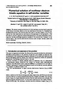
Then, applying lemma 3.4, with α = 2/3, φ = C4 h4/3 and χ = C5 h, yields ! Ã h4/3 (50) |ei | ≤ C C4 2/3 + C5 h . ti ¤ 4. Numerical results. Equation (7) was solved by the Euler’s method (20) and table 1 contains approximations of y(t) obtained with several values of the stepsize. In table 2 we have computed experimental rates of convergence. The following quantity has been used as an estimate of the convergence order µ h/2 ¶ y − yh log y h/4 − y h/2 p≈ , log 2 where y h , y h/2 and y h/4 denote approximations to y(t) using the mesh spacings h, h/2 and h/4, respectively. The results of table 2 indicate first order of convergence, which is in agreement with the result (48) of theorem 3.2. This is also illustrated in figure 1, where the absolute errors for N = 160, 320, 640 are shown. In order to obtain error estimates we have taken y 1/1280 as the exact solution of equation (7). The computed error norms, given by: 1/N

keN k∞ = max |y(ti ) − yi 1≤i≤N

|,

ti =

i , N

are displayed in table 3, together with the corresponding rates of convergence. The numerical results suggest that the global order of convergence is 1/3, confirming the theoretical result (38).

10


Error 0.0008 h=1160 0.0006 h=1320 0.0004 h=1640

0.0002 0

0.2

0.4

0.6

0.8

1

x

Figure 1. Absolute errors for Euler’s method

ti 0 0.1 0.2 0.3 0.4 0.5 0.6 0.7 0.8 0.9 1.0

N=80 1 0.835743 0.78719 0.757239 0.735494 0.718428 0.704395 0.692489 0.682160 0.673046 0.664895

Table 1 Approximations of y(t) N=160 N=320 N=640 1 1 1 0.83471 0.834191 0.833937 0.786799 0.786600 0.786502 0.757030 0.756924 0.756871 0.735366 0.735299 0.735267 0.718342 0.718297 0.718275 0.704334 0.704302 0.704287 0.692445 0.692422 0.692411 0.682127 0.682110 0.682102 0.673021 0.673008 0.673001 0.664876 0.664866 0.664861

N=1280 1 0.833814 0.786454 0.756846 0.735251 0.718265 0.704280 0.692406 0.682098 0.672998 0.664859

Table 2 Convergence rates for several values of N ti 160,320,640 320,640,1280 0.1 1.121 1.088 0.2 1.080 1.061 0.3 1.062 1.048 0.4 1.052 1.041 0.5 1.045 1.035 0.6 1.040 1.032 0.7 1.036 1.029 0.8 1.033 1.026 0.9 1.030 1.024 1.0 1.028 1.023 Table 3 Errors and convergence N h kek∞ 40 0.025 0.123577 80 0.0125 0.088151 160 0.00625 0.059719 320 0.003125 0.037638 640 0.0015625 0.020352

rates rate 0.1766 0.2491 0.3173 0.3647 0.3532


Table 4 Errors and convergence for equation (5) N h kek∞ 40 0.025 0.00463 80 0.0125 0.00201 160 0.00625 0.000878 320 0.003125 0.000360 640 0.0015625 0.000116

11

rates rate − − 1.208 1.128 1.089

5. Conclusions and future work. We have introduced a nonlinear Volterra integral equation with an Abel type kernel of the form p(t, s, y(s))(t − s)−α , where α = 2/3 and p(t, s, y) = s1/3 y 4 (cf. (7)). We have shown that, while near the origin the exact solution y(t) behaves like t2/3 , it is differentiable if t is large enough. Numerical approximations to y were obtained by Euler’s method and shown to be convergent of order 1/3. Moreover it was proved that, for t away from the origin, the convergence order is one. These results were confirmed by some numerical examples. For the sake of comparison, we have also included in table 4 the error norms and convergence rates for Euler’s method applied to equation (5). The obtained estimates are in agreement with the predicted first order of convergence. In future work we shall investigate the application of the techniques used in this paper to a general class of equations with kernel sγ y(s)n (t − s)−α , where 0 < α, γ < 1. The use of graded meshes as well as higher order methods will also be considered. 6. Acknowledgements. The authors are pleased to acknowledge financial support from Funda¸c˜ao para a Ciˆencia e Tecnologia (Project POCTI/MAT/45700/2002). REFERENCES [1] H.Brunner, ”Collocation methods for Volterra integral and related functional differential equations integral”, Cambridge University Press (2004). [2] H.Brunner, P.J.van der Houwen, ”The numerical solution of Volterra integral equations”, CWI Monographs 3, Amsterdam, (1986). [3] H.Brunner, A.Pedas, G.Vainikko, The piecewise polynomial collocation method for nonlinear weakly singular Volterra equations, Math. Comp., 68 (1999), 1079-1095. [4] J.Dixon, On the order of the error in discretization methods for weakly singular second kind Volterra integral equations with non-smooth solutions, BIT 25 (1985) 624-634. [5] J.Dixon, S.McKee, Weakly singular discrete inequalities, ZAMM, 66 (1986) 535-544. [6] N.M.B.Franco, S.McKee, A family of high order product integration methods for an integral equation of Lighthill, Int. J. Comput. Math. 18 (1985) 173-184. [7] N.B.Franco, S.McKee, J.Dixon, A numerical solution of Lighthill’s equation for the surface temperature distribution of a projectile, Mat. Aplic. Comp., 12 (1983) 257-271. [8] J.M.Lighthill, Contributions to the theory of the heat transfer trough a laminar boundary layer, Proc. Roy. Soc. London, 202A (1950) 359-377. [9] Ch.Lubich, Runge-Kutta theory for Volterra and Abel integral equations of the second kind, Math. Comp., 41 (1983), 87-102. [10] R.Miller, ”Nonlinear Volterra Integral Equations, W.A.Benjamin, California (1971). [11] R.K.Miller, A.Feldstein, Smoothness of solutions of Volterra integral equations with weakly singular kernels, SIAM J. Numer. Anal., 2 (1971) 242-258. [12] B.Noble, The numerical solution of nonlinear integral equations and related topics, Anselone, (1964). E-mail address: [email protected] E-mail address: [email protected] E-mail address: [email protected]