Numerical Solutions of Differential and Delay

Numerical Solutions of Differential and Delay Differential Equations Stephen A. Wirkus

Arizona State University

Background

• Continuous, deterministic models are easiest to obtain information analytically • Even in these cases, we cannot always analytically solve the given equation or system of equations • Numerical solutions of the system of differential equations are often needed and/or used to confirm the qualitative predictions • Many numerical methods exist: implicit or explicit, one-step or multi-step, fixed step-size or variable step-size; all are characteristics that one can use

Consider x0 = f (t, x), x ∈ R1

(1)

Example: x0 = rx(1 − x), the logistic equation, can be solved exactly using separation of variables and a partial fractions expansion. 2

Example: x0 = e−x cannot be solved exactly in terms of elementary functions because the integral Z 2

ex dx cannot be evaluated as an indefinite integral.

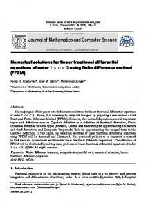
Analytically we are trying to find a function (the solution) x(t) such that x(t) satisfies x0 = f (t, x) for t ∈ (a, b). We don’t know this solution beforehand but we do know its derivative—it’s just the right-hand-side of (1), f (t, x). In other words, the solution has slope f (t, x) which is always given. We can use the direction field (or slope field) to find the approximate numerical solution. To each point in the t-x plane we associate an arrow with slope f (t, x). direction field

direction field & soln

1.6

1.6

1.5

1.5

1.4

1.4

y(x) 1.3

y 1.3

1.2

1.2

1.1

1.1

1

1 0

0.2

0.4

0.6 x

0.8

1

0

0.2

0.4

0.6 x

0.8

1

How could we graph such a solution if we didn’t have the explicit formula? One of the simplest ways is to use Euler’s Method. Consider x0 = f (t, x) and suppose we are at the point (ti , xi ). For a stepsize h, the approximate solution at ti + h is denoted xi+1 where xi+1 = xi + hf (ti , xi ).

Accuracy of Euler Method

Let the exact solution at ti + h be denoted x(ti + h). The hope is that xi+1 and x(ti + h) are close to each other. For Euler’s method we have |xi+1 − x(ti + h)| ≤ Ch

for some constant C. The approximation is thus better, in theory, for smaller h values. In practice, an extremely small h gives rise to an enormous amount of computational work and gives rise to the accumulation of roundoff errors.

Accuracy of Euler Method

• Many other methods exist that are far better than (forward) Euler’s Method • Explicit and implicit methods; one-step and multi-step methods; fixed stepsize and variable stepsize methods • All have their good and bad points • The most commonly used method in practice is the 4th order Runge-Kutta method (we’ll denote it as RK4) or slight variations of it

Accuracy of 4th order Runge-Kutta

Let the exact solution at ti + h be denoted x(ti + h). • For the RK4 method,

|xi+1 − x(ti + h)| ≤ Mh4

• More computations to perform at each step but the h4 bound is worth it • RK4 uses uses the current slope at (ti , xi ) as well as two slopes at ti + ti + h

h 2

and one at

1. First evaluation k1 = f (ti , xi ) • Calculate slope of solution passing through current value (ti , xi ), call it k1 . • Euler’s method continues at this slope for one step size and the Euler approximation of the next value is (ti + h, xi + hk1 ). • RK4 takes half of this increase in the x coordinate, and goes to the t-value halfway between ti and the next step ti + h.

2. Second evaluation k2 = f (ti + h2 , xi +

hk1 ) 2

hk

• The “mid-value" t-value is the halfway point ti + h2 and the x-value is xi + 21 . • Evaluate slope of the solution passing through this point, call it k2 . • Take half of the increase and go back to the “mid-value" t-value and a different hk x-value, xi + 22 .

hk

3. Third evaluation k3 = f (ti + h2 , xi + 22 ) • The “mid-value" t-value is still the halfway point ti + hk2 . 2

h 2

and the x-value is now

xi + • Evaluate the slope of the solution passing through this point, call it k3 . ) gives x-value of • Following this slope for one step size (to the t-value ti + 3h 2 xi +

hk2 2

+ hk3 .

4. Fourth evaluation k4 = f (ti + h, xi + hk3 ) • Then calculate the slope of the solution which passes through the value (ti + h, xi + hk3 ). Call this slope k4 . • Note that the (t, x) value where we evaluate at is not the original one predicted by Euler’s Method.

The four steps of RK4

Let (ti , xi ) be the current point. Then xi+1 = xi + is the approximate solution at ti + h.

h
k + 2k2 + 2k3 + k4 6 1

Example: Use Euler’s method and the 4th order Runge-Kutta method with h = 0.1 to approximate the solution of dx = tx dt with x(0) = 1 on 0 ≤ t ≤ 1. Determine the exact solution and compare the results. Answer: We have f (t, x) = tx. The initial condition x(0) = 1 says that t0 = 0 and x0 = 1 so with h = 0.1 we have t1 = t0 + h = 0.1, · · · , t10 = t0 + 10h = 1.0. The exact solution to

dx = tx dt with the condition x(0) = 1 is found using separation of variables to be x(t) = et

2

/2

ti 0.0 0.1 0.2 0.3 0.4 0.5 0.6 0.7 0.8 0.9 1.0

Euler xi 1.0 1.0 1.01 1.0302 1.06111 1.10355 1.15873 1.22825 1.31423 1.41937 1.54711

Exact x(ti ) 1.0 1.0050 1.0202 1.0460 1.08329 1.13315 1.19722 1.27762 1.37713 1.49930 1.64872

Error |xi − x(ti )| 0 0.005 0.0102 0.0158 0.02218 0.02960 0.03849 0.04937 0.06290 0.07993 0.10161

ti 0.0 0.1 0.2 0.3 0.4 0.5 0.6 0.7 0.8 0.9 1.0

RK4 xi 1.0 1.005012 1.020201 1.046027 1.083287 1.133148 1.197216 1.277621 1.377127 1.499302 1.648721

Exact x(ti ) 1.0 1.005013 1.020201 1.046028 1.083287 1.133148 1.197217 1.277621 1.377128 1.499303 1.648721

Error |xi − x(ti )| 0.0 0.000001 0.000000 0.000001 0.000000 0.000000 0.000001 0.000000 0.000001 0.000001 0.000001

RK4.m in Matlab function [xout,yout]=RK4(fname,xvals,y0,h) %fname = the function f for the equation. %xvals =vector with initial x0 and final xf %y0 =initial y, h =stepsize x0=xvals(1); xf=xvals(2); xn=x0; yn=y0; xout=xn; yout=yn; fn=feval(fname,xn,yn); steps=(xf-x0)/h for j=1:steps [xn,yn,fn]=RK4step(fname,xn,yn,fn,h); xout=[xout; xn]; yout=[yout; yn]; end % % % % % % % % % % % % % % % % % % % % % % % % % function [xnout,ynout,fnout]=RK4step(fname,xn,yn,fn,h) % The next value of the approximate solution is given by (xnout,ynout) and the slope of the solution through that point is thus f(xnout,ynout). yn=yn’; k1 = h*fn; k2 = h*feval(fname,xn+(h/2),yn+(k1/2)); k3 =h*feval(fname,xn+(h/2),yn+(k2/2)); k4 = h*feval(fname,xn+h,yn+k3); ynout = yn +(k1 + 2*k2 + 2*k3 + k4)/6; xnout = xn+h; fnout = feval(fname,xnout,ynout); ynout=ynout’; % end of m-file RK4.m % In the command window, we would type % % [x,y]=RK4(@Example,[0,1],1,.1); % [x y] % to see the numerical values % plot(x,y) % to see the graphical solution

• Most models will be fine with RK4.m (or a variation of it) • Easy to implement • The code is analogous for more equations—just consider the original system x0 = f (t, x) where now x ∈ Rn • Incorporating a variable stepsize is a natural improvement • Easily modified for models that include a time delay

Model with Delayed Recruitment

Non-delay model x0 (t) = R(x(t)) − µx(t) where µ > 0, R(0) = 0, R0 (0) = r > 0 and R(x) is bounded for large x. People are recruited into a class based on information that they have. This information is not about the current state of the system but the system τ time units before since information is not disseminated/ known instantaneously. Delay Model x0 (t) = R(x(t − τ)) − µx(t)

Fitzhugh-Nagumo equations • v represents the membrane potential • ω represents the recovery or hyperpolarization of neuronal action potential (potassium gating, leakage currents, and ATP pump action).

dv dt dω dt

=

v(a − v)(v − 1) − ω + I

=

ε(v − γω)

(2)

Consider the effect of alcohol on the brain. A system proposed by Franca, et al. models alcohol as causing a neuronal communication delay. Thus there will be a delay in the restoring force. dv dt dω dt

=

v(v − 1)(a − v) − ω(t − τ) + I

=

ε(v − γω)

(3)

Coupled Microwave Oscillators

¨x1 + x1 − ε (1 − x12 ) ˙x1

=

ε α˙x2 (t),

(1 − x22 ) ˙x2

=

ε α˙x1 (t)

¨x2 + x2 − ε

(4)

α is a coupling parameter, ε is the nonlinearity. • Oscillators typically operate around 10 GHz ⇒ Period ∼ 102π10 ∼ 6 × 10−10 sec cm • Speed of light: 3 × 1010 sec • In one period, light travels ∼ (6 × 10−10 ) × (3 × 1010 ) = 18cm • If oscillators are, say 4cm apart, the received signal is delayed ∼ 14 period. • Delayed velocity coupling occurs in radiatively coupled microwave osillator arrays.

¨x1 + x1 − ε (1 − x12 ) ˙x1

=

ε α˙x2 (t − τ),

(1 − x22 ) ˙x2

=

ε α˙x1 (t − τ)

¨x2 + x2 − ε τ is the delay time

(5)

Initial Conditions Let (ti , xi ) represent the current state of the system and denote the system x˙(t) = f(t, x(t), x(t − τ)).

(6)

In all the cases with time delay, the next step of the system will depend not only on the current information but also on the state of the system τ time units ago. We first need to find a solution of the form x(t) = Φ(t), t0 − τ ≤ t ≤ t0

(7)

We can then use these values to calculate the solution of x(t) for t0 + τ ≤ t ≤ t0 + 2τ. One method to generate this interval of initial conditions considers the equation without the delay and lets them run backward in time until t = −τ. Then begin numerically integrating the delayed equations, taking into account what happened τ units ago.

Modified Runge-Kutta Here we use a fourth order Runge-Kutta scheme with fixed step size, appropriately modified to account for delay. For the case of delay, our system is of the form ˙x = f (t, x(t), x(t − τ)) and we use the notation Φn− τ ≡ x(tn − τ) to denote the value of the system τ time h units ago (and we assume for convenience that hm = τ, for some integer m). We now must evaluate   k1 = hf tn , xn , Φn− τ , h ‚ Œ h k1 Φn− τh + Φn+1− τh k2 = hf tn + , xn + , , 2 2 2 ‚ Œ h k2 Φn− τh + Φn+1− τh k3 = hf tn + , xn + , , 2 2 2   k4 = hf tn + h, xn + k3 , Φn+1− τ h

where Φn+1− τ is the system τ time units before xn+1 . h

Some considerations • The evaluation of k2 , k3 requires an evaluation of x(t) at the midpoint between tn − τ and tn+1 ≡ tn + h − τ. We take the average of the known delayed values Φn− τ , Φn+1− τ , which is the function value between tn− τ and h h h t n+ 1− τ . h

• At each step, we need the approximate solution of the system τ time units ago and thus need to carry around the solution vector on [xi − τ, xi ]. • For example, if τ = 2, h = .01, we would need to keep a vector of length 200. • For large delay, storage might be an issue. • This is sometimes dealt with by looking at a ratio of stepsize to delay length.

Runge-Kutta Modified for Delay

Runge-Kutta Modified for Delay

Plus two other analogous evaluations.

More considerations

• There is not only one way to generate the interval of initial conditions • For example, in the microwave oscillator model, it might be better to generate the IC by running the system backward uncoupled (as opposed to backward and couple) • The approach of a solution to a stable steady-state solution might depend on this generated IC • Variable stepsize will be more difficult to analyze because we may have to interpolate between values close to τ time units ago since it’s possible that the system “skipped over" those points.

Delay code for Fitzhugh-Nagumo equations function [tvals,yvals]=alcohol(t0,tf,y0,gam,cur) global a epsilon gamma I1 a=.139; epsilon=.008; gamma=gam; I1=cur; peek=10; h=.01; tau=1/(gamma*epsilon); n=round((tf-t0)/h); tc=t0; yc=y0; yp=yc; tvals=tc; ypvals=yc; fc=feval(’derivs’,tc,yc);delsteps=round(tau/h); for i=1:delsteps % integrate backward w/o delay to generate IC [tc,yp,fc]=RKstep(’derivs’,tc,yp,fc,-h); ypvals=[yp ypvals]; tvals=[tc tvals]; end tc=t0; yp=ypvals; fcp=feval(’derivsdel’,tc,yc,yp(:,1)); yvals=yp; % the system at time (t-tau) is the first column of yp if (n>delsteps) yvals=yc; tvals=tc; end for j=1:n % integrate forward w/ delay [tc,yc,fcp]=RKdelstep(’derivsdel’,tc,yc,yp,fcp,h); if mod(j,peek)==0 yvals=[yvals yc]; tvals=[tvals tc]; end yp=[yp(:,2:delsteps+1) yc]; end

%************************************* function [tnew,ynew,fnew]=RKdelstep(fname,tc,yc,yp,fcp,h) ya=yp(:,1); ya1=0.5*(yp(:,1)+yp(:,2)); ya2=yp(:,2); k1 = h*fcp; k2 = h*feval(fname,tc+(h/2),yc+(k1/2),ya1); k3 = h*feval(fname,tc+(h/2),yc+(k2/2),ya1); k4 = h*feval(fname,tc+h,yc+k3,ya2); ynew = yc +(k1 + 2*k2 + 2*k3 +k4)/6; tnew = tc+h; fnew = feval(fname,tnew,ynew,yp(:,2)); %************************************** function [tnew,ynew,fnew]=RKstep(fname,tc,yc,fc,h) k1 = h*fc; k2 = h*feval(fname,tc+(h/2),yc+(k1/2)); k3 = h*feval(fname,tc+(h/2),yc+(k2/2)); k4 = h*feval(fname,tc+h,yc+k3); ynew = yc +(k1 + 2*k2 + 2*k3 +k4)/6; tnew = tc+h; fnew = feval(fname,tnew,ynew); %************************************** function dy=derivsdel(tc,yc,ya) global a epsilon gamma I1 v=yc(1); w=yc(2); vt=ya(1); wt=ya(2); dy=[-v*(v-1)*(v-a)-wt+I1; epsilon*(v-gamma*w)]; %************************************** function dy=derivs(tc,yc) global a epsilon gamma I1 ya=yc; v=yc(1); w=yc(2); vt=ya(1); wt=ya(2); dy=[-v*(v-1)*(v-a)-wt+I1; epsilon*(v-gamma*w)];

Example 1:  π‹ x0 (t) = −x t − , x(t) = sin t for t ∈ [−π/2, 0] 2

has solution x(t) = sin t. ti Exact x(ti ) 0 0 0.523 0.50000000 1.047 0.86602540 1.570 1.00000000 2.094 0.86602540 2.617 0.50000000 3.141 0.00000000

RK4d xi 0 0.49999543 0.86601748 0.99999086 0.86601871 0.49999999 0.00000913

Error |xi − x(ti )| 0 -0.00000456 -0.00000791 -0.00000913 -0.00000668 -0.00000000 0.00000913

Example 2: x0 (t) = e · x(t − 1), x(t) = et for t ∈ [−1, 0] has solution x(t) = et . ti Exact x(ti ) 0 1.00000000 0.50 1.64872127 1.00 2.71828182 1.50 4.48168907 2.00 7.38905609 2.50 12.18249396 3.00 20.08553692

RK4d xi 1.00000000 1.64872667 2.71829614 4.48172145 7.38912561 12.18263349 20.08580883

Error |xi − x(ti )| 0 0.00000540 0.00001431 0.00003238 0.00006951 0.00013953 0.00027191

Non-Delay: Explicit vs. Implicit Methods Both (forward) Euler and Runge-Kutta methods are known as explicit methods. That is, everything on the right-hand side is known and only the left-hand side is unknown: xi + hf (ti , xi ) (forward Euler) (8) h
k + 2k2 + 2k3 + k4 (RK4) (9) xi+1 = xi + 6 1 A simple modification can give us an implicit method, which is often more accurate. In this situation, we have a formula in which xi+1

=

xi+1 = xi + hf (ti+1 , xi+1 )

(backward Euler)

Thus in order to calculate the right-hand side, we need to know the left-hand side! For simple equations, we can actually solve the formula and make the method explicit. If not, we often combine the implicit method with an explicit method and obtain what is called a predictor-corrector method: 1. Predict xi+1 with forward Euler: xi+1 = xi + hf (ti , xi ) 2. Substitute this prediction into the implicit backward Euler formula: xi+1 = xi + hf (ti+1 , xi+1 ) 3. Repeat, using the result from 2 as your new “prediction."

Non-Delay: Single-step vs Multistep Euler used only the knowledge of the current point to calculate the next value of the approximate solution whereas RK4 used the current point plus the previous one plus 2 intermediate interpolations to calculate the next value. Numerical methods that use more than the current point to calculate the next value are called multistep methods. A simple explicit multistep method, known as the 2nd order Adams-Bashforth method, is xi+1 = xi +

h
3f (ti , xi ) − f (ti−1 , xi−1 ) , 2

i = 1, 2, · · · , N − 1,

(10)

5 (3) x (xii )h2 , for some ξi ∈ (ti−2 , ti+1 ). with local truncation error 12 It is often used with an implicit method Adams-Moulton:

xi+1 = xi +

h
5f (ti+1 , xi+1 ) + 8f (ti , xi ) − f (ti−1 , xi−1 ) , 12

(11)

i = 1, 2, · · · , N − 1, The local truncation error is given by −241 x(4) (ξi )h2 , for some ξi ∈ (ti−1 , ti+1 ). Together we have a more accurate (than Euler) predictor corrector method to approximate a numerical solution. These predictor-corrector methods are often used when solutions change rapidly in places (e.g., stiff equations).

Multistep Predictor-Corrector Methods in Delay We presented a modified Runge-Kutta method for dealing with delay. We can control the accuracy better than by using MATLAB’s dde23. Other modifications exist. Yeung uses multipoint sixth-order Adams-Bashforth-Moulton predictor/ corrector method with fixed stepsize dt = τ/20, tmax = 1000τ. This might be desirable if the number of equations is large since the fourth order Runge-Kutta method requires four function evaluations at each time step. The entire interval of the state of the system from now to τ time units ago still needs to be kept. 6th order Adams-Bashforth (explicit method, predictor): h (4277fi − 7923fi−1 + 9982fi−2 xi+1 = xi + 1440 −7298fi−3 + 2877fi−3 + 2877fi−4 − 475fi−5 ) 6th order Adams-Moulton (implicit method, corrector): h xi+1 = xi + (475fi+1 + 1427fi − 798fi−1 + 482fi−2 − 173fi−3 + 27fi−4 ) 1440

Your Homework Modify the fourth-order Adams-Bashforth-Moulton method to incorporate a fixed delay, τ: h (55fi − 59fi−1 + 37fi−2 − 9fi−3 ) Adams-Bashforth predictor: xi+1 = xi + 24 xi+1

=

xi +

h (55f (ti , xi , Φ(ti − τ)) − 59f (ti−1 , xi−1 , Φ(ti−1 − τ)) 24 +37f (ti−2 , xi−2 , Φ(ti−2 − τ)) − 9f (ti−3 , xi−3 , Φ(ti−3 − τ)))

h Adams-Moulton corrector: xi+1 = xi + 24 (9fi+1 + 19fi − 5fi−1 + fi−2 )

xi+1

=

xi +

h (9f (ti+1 , xi+1 , Φ(ti+1 − τ)) + 19f (ti , xi , x(ti − τ)) 24 −5f (ti−1 , xi−1 , Φ(ti−1 − τ)) + f (ti−2 , xi−2 , Φ(ti−2 − τ)))

Compare with x0 (t) = e · x(t − 1), x(t) = et for t ∈ [−1, 0] from Example 2: ti 0 0.50 1.00 1.50 2.00 2.50 3.00

Exact x(ti ) 1.00000000 1.64872127 2.71828182 4.48168907 7.38905609 12.18249396 20.08553692

RK4d xi 1.00000000 1.64872667 2.71829614 4.48172145 7.38912561 12.18263349 20.08580883

Error |xi − x(ti )| 0 0.00000540 0.00001431 0.00003238 0.00006951 0.00013953 0.00027191

Conclusions • Multistep methods are often used to numerically solve PDEs (e.g., “Stability and Convergence of the Crank-Nicolson/Adams-Bashforth Scheme for the Time-Dependent Navier-Stokes Equations,” by Yinnian He and Weiwei Sun, SIAM Journal on Numerical Analysis, 2007, Vol. 45 Issue 2, p837-869). • There are also software packages that address bifurcation issues in delay equations (e.g., “Numerical Bifurcation Analysis of Delay Differential Equations Using DDE-BIFTOOL,” by K. Engelborghs, T. Luzyanina, D. Roose, ACM Transactions on Mathematical Software, Mar 2002, Vol. 28 Issue 1). • DDE-BIFTOOL: a Matlab package for bifurcation analysis of delay differential equations (2000) http://citeseerx.ist.psu.edu/viewdoc/summary?doi=10.1.1.36.1399

Conclusions

• Differential Delay Equations arise naturally in numerous physical and biological systems • Important to understand non-delay numerical methods before trying to modify them to account for delay • Numerous methods exist; each has its benefits and drawbacks • In practice, make sure you have a way to check your code on an example with a known solution before exploring those that you don’t know • For a given problem, try to think of the most natural way to generate the interval of initial conditions.

References Richard L. Burden and J. Douglas Faires, Numerical Analysis, Brooks/Cole, Pacific Grove, 2001. Franca,R., Prendergast,I., Sanchez,E., Sanchez,M., and Berezovsky,F., The Role of Time Delay in the Fitzhugh-Nagumo Equations: The Impact of Alcohol on Neuron Firing Department of Biometrics Technical Report, Cornell University, 2001. Hairer, E., Nørsett, S. P., and Wanner, G., Solving Ordinary Differential Equations I: Nonstiff Problems, Springer-Verlag, Berlin, 1987. W. Press, S. Teukolsky, W. Vetterling and B. Flannery, Numerical Recipes in C: The art of scientific computing, Cambridge, 1995. Swift,R. and Wirkus,S., A Course in Ordinary Differential Equations, Taylor & Francis, 2006. Wirkus,S. The dynamics of two coupled van der Pol oscillators with delay coupling Ph.D.thesis, Center for Applied Mathematics, Cornell University, 1999. Yeung,M.K.S. Time delay in the Kuramoto model of coupled oscillators, Ph.D.thesis, Dept.of Theoretical and Applied Mechanics, Cornell University, 1999.