Singly Diagonally Implicit Runge-Kutta (SDIRK) method is used to solve (3) at the point ... here is DDE which has a single delay, both time dependent and state.
Matematika, 2002, Jilid 18, Bil. 2, hlm. 79–90 c
Jabatan Matematik, UTM.
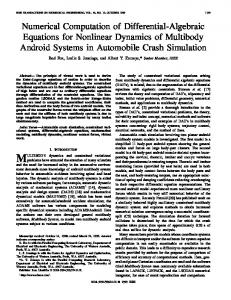
Numerical Treatment of Delay Differential Equations by Runge-Kutta Method Using Hermite Interpolation Fudziah Ismail, Raed Ali Al-Khasawneh, Aung San Lwin & Mohamed Suleiman Department of Mathematics, Universiti Putra Malaysia, 43400 UPM, Serdang, Malaysia. Abstract Embedded Diagonally Implicit Runge-Kutta methods of different orders are used for the treatment of delay differential equations. The delay argument is approximated using an appropriate Hermite Interpolation. The numerical results based on these methods are compared and the Q-stability region of the methods are presented.
1
Introduction
In the last two decades there has been a growing interest in the numerical treatment of delay differential equations (DDEs). This is due to their versatility in the mathematical modeling of processes in various application fields. DDEs generally provide the best and sometimes the only realistic simulation of observed phenomena. Such work can be found in Orbele and Pesch (1981), Baker and Paul (1992) and Zennaro (1988). First order DDE can be written as y 0 (t) y(t)
= f (t, y, y(t − τ )) = ϕ(t) t ≤ t0
t > t0 (1)
if it has one delay term only, or y 0 (t)
= f (t, y, y(t − τ1 ), . . . y(t − τn ))
y(t)
= ϕ(t)
t ≤ t0
t > t0 (2)
if it has more than one delay term. ϕ(t) is the initial function, τ (t, y(t)) is called the delay, is called the delay argument, the value of y(t − τ (t, y(t)) is the solution of the delay term or commonly referred to as the
Fudziah Ismail, Raed Ali Al-Khasawneh, Aung San Lwin & Mohamed Suleiman
80
delay term only. If the delay is a constant then it is called constant delay, if it is function of time t, then it is called time dependent delay, if it is a function of time t and y(t) then it is called the state dependent delay.
2
Numerical Treatment Of DDEs Most numerical methods for solving ordinary differential equation of the form y 0 (t) = f (t, y(t))
y(t0 ) = c
(3)
can be adapted to solve DDEs. The range comprises of one step methods such as RungeKutta method and Euler method, multistep and also block implicit method. When a q-stage Singly Diagonally Implicit Runge-Kutta (SDIRK) method is used to solve (3) at the point tn+1 , the following equations will be obtained: k1 = f (tn + c1 h, yn + ha11 k1 ) k2 = f (tn + c2 h, yn + ha21 k1 + ha22 k2 ) .. . i X aij kj ) ki = f (tn + ci h, yn + h j=1
yn+1
= yn + h
q X
bi ki
(i = 1, . . . , q)
i=1
yn + h
i X
aij kj is called the internal stage of the method.
j=1
When it is adapted to DDE(1) we have ki
= f (tn + ci h, yn + h
i X
aij kj , y(tn + ci h − τ ))
j=1
yn+1
= yn + h
q X
bi ki
i=1
y(tn + ci h − τ ) is the delay term and interpolation is needed to approximate the value. There are a number of techniques for obtaining the approximations which has been discussed in Neves (1981), In’t Hout (1992) and Karoui (1992). In this paper Hermite interpolation is used to approximate the delay term. The interpolation order and hence the number of support points have to be adapted to the order of the method. If p denotes the order of the Runge-Kutta method used, the interpolation order q must be greater or equal to p. Let ip denotes the number of support points for Hermite interpolation then 2ip > p (4)
Numerical Treatment of Delay Differential Equations
81
In this paper fifth order embedded (SDIRK) method (4,5) in (5,6) (see Ismail and Suleiman (1999)) and fourth order embedded SDIRK (3,4) in (4,6) due to Hairer and Wanner (1991) were used to solve DDEs. For the fifth order method three support points were used, so that equation (4) holds and for the fourth order method we are also using three support points since if two support points were used the order of the interpolations is less than the order of the method itself. In the numerical treatment of delay differential equations two essential difficulties occur. First is the evaluation of the delay term which has been discussed earlier and secondly is the jump discontinuities of the solution in various derivatives, which usually are the characteristic of DDEs. When solving DDEs, one of the basic requirements is the storage of sufficient back information so that the method can evaluate the delay term when it is required at some point t ≤ tn . The amount of information to be stored at each time step depends on the method for approximating the delay term, but the interval on which the information is to be stored and the quantities to be stored on that interval should be flexible and adaptable for each problem, depending on the nature of the delay term and accuracy required. If the delay term falls at some point t ≤ t0 , then the initial function must be used. The delay argument may fall in the current step because it is smaller than the stepsize or may even vanish, we call this type of delay a small delay or when the delay vanishes we call it vanishing delay. These types of delays are handled by either restricting the stepsize to be smaller than the delays or using extrapolation. Discontinuities are handled by the error control mechanism or locating the discontinuity points by solving associated nonlinear equations. In this paper the test equations used have the analytical solution so we knew the discontinuity point hence make it a mesh point so that the stepsize does not cross the discontinuity point. The main concern here is DDE which has a single delay, both time dependent and state dependent and of the large type.
3
Stability Of The Method
There are many concepts of stability of numerical methods when applied to DDE, depending on the test equation as well as the delay term involved see Bellen et al., (1988), Tian Hongjiang and Kuang Jiaoxun (1995) and Guang-Da Hu and Meguid, S. A. (1999). One of the most commonly used test equation in the literature is, y 0 (t) y 0 (t)
= λy(t) + µy(t − τ ), = ϕ(t), t ≤ t0
t ≥ t0 (5)
λ and µ ∈ C, τ > 0 and ϕ is continuous. If λ = 0, the following equation is obtained y 0 (t) 0
y (t)
= µy(t − τ ) = ϕ(t)
t ≥ t0
t ≤ t0
Barwell (1975) introduced the following concept of stability.
(6)
Fudziah Ismail, Raed Ali Al-Khasawneh, Aung San Lwin & Mohamed Suleiman
82
Definition: Given a numerical method for DDEs, the P-stability region of the method is the set Sp of pairs of (α, β), such that the numerical solution of (5) asymptotically vanishes for steplengths h satisfying h=
τ , m
m
is a positive integer.
Definition: If µ ∈ C, Q-stability region of the method is the set SQ of β, such that the numerical solution of (6) asymptotically vanishes for steplengths h satisfying h=
τ , m
m
is a positive integer.
α = hλ and β = hµ. When q-stage Runge-Kutta method is applied to DDE (5), using Hermite interpolation for the delay term, the following equations are obtained. (i)
kn+1
= f (tn + ci h, yn + h
i X
(j)
aij kn+1 +
X
¯ i )hy 0 H(ci )yn−m+l + H(c n−m+l )
j=1
yn+1
= yn + h
q X
(i)
bi kn+1
(7)
i=1
¯ are the coefficients of Hermite interpolation. Where H and H Define u = (1, . . . , 1)T and for n ≥ 1 kn b Hl (c) ¯ l (c) H
T = (kn(1) , . . . , k(q) n ) T = (b1 , b2 , . . . , bq )
= Hl (c1 ), . . . , Hl (cq ) ¯ l (c1 ), . . . , H ¯ l (cq ) = H
For n ≥ m (7) takes the form
kn+1 = λ(yn u + hAkn+1 ) + µ
s X
¯ l (c)yn−m+l + hH ¯ l (c)y 0 (Hl (c)yn−m+l + hH n−m+l ) (8)
l=r
yn+1 = yn + hbT kn+1
(9)
0 by λyn−m+l + µyn−2m+l , we will have Replacing yn−m+l
kn+1 = λyu + hλAkn+1 + µ
s X
Hl (c)yn−m+l + µhλ
l=r
s X l=r
¯ l (c)yn−m+l + hµ2 H
s X
¯ l (c)yn−2m+l H
l=r
hence, we have
(I − hλA)kn+1 = λyn u + µ
s X � � ¯ l (cc))yn−m+l + hµH(c) ¯ l yn−2m+l (Hl (c) + hλH l=r
Numerical Treatment of Delay Differential Equations
hkn+1
83
= hλ(I − hλA)−1 yn u + s X � � −1 ¯ l (c))yn−m+l + hµH(c) ¯ l yn−2m+l (10) (Hl (c) + hλH hµ(I − hλA) l=r
replacing the above equation into (9) and taking α = hλ, β = hµ and η = (I − hλA)−1 we have
yn+1 = yn + αbT ηyn u + βbT η
s X � � ¯ l (c))yn−m+l + hµH(c) ¯ l yn−2m+l (Hl (c) + hλH
(11)
l=r
Rewriting Yn+1 =
� yn+1 , hkn+1
�
equation (10) can be written as � � � � � T P ¯ l (c)) 1 0 1 + αbT ηu 0 βb ηP Hl (c) + λH Y + Yn+1 = ¯ l (c)) 0 I αηu u n βη Hl (c) + αH � � 2 T P ¯ l (c) 0 β b ηP H Y ¯ l (c) β2η H 0 n−2m+l
� 0 Y + 0 n−m+l
I is the identity matrix, replacing Y by ζ, the stability polynomial of the method is � � � � T P ¯ l (c)) 1 + αbT ηu 0 n βb ηP Hl (c) + λH 1 0 n+1 ζ − ζ − S(α, β, ζ) = det[ ¯ 0 I αηu u βη Hl (c) + αHl (c)) � � 2 T P ¯ l (c) 0 n−2m+l β b ηP H ζ − ] ¯ l (c) β2η H 0 �
� 0 n−m+l ζ 0
Hence
S(α, β, ζ)
= ζ n+1 − (1 + αbT ηu)ζ n − βbT η 2 T
− β b η
X
X ¯ l (c))ζ n−m+l (Hl (c) + λH l
¯ l (c)ζ H
n−2m+l
(12)
l
The above polynomial is called the P -stability polynomial of the method using Hermite interpolation to approximate the delay term. If λ = 0, hence α = 0, then we obtain X X ¯ l (c)ζ n−2m+l (Hl (c))ζ n−m+l − β 2 bT η (13) S(β, ζ) = ζ n+1 − ζ n − βbT η H l
that is the Q-stability polynomial of the method.
l
Fudziah Ismail, Raed Ali Al-Khasawneh, Aung San Lwin & Mohamed Suleiman
84
By taking n − 2m − 1 = 0, so that the lowest order of ζ is zero and using three points for the interpolations for both the methods we have three values of y and y 0 , that is six data altogether so that the interpolations are at least of the same order as the method. Hermite polynomial of least degree agreeing with y and y 0 at t0 , . . . , tn is a polynomial of degree at most 2n + 1 given by P2n+1 (t)
=
n X
Hn,j (t)y(tj ) +
j=0
n X
¯ n,j (t)y 0 (tj ) H
j=0
where Hn,j (t) ¯ n,j (t) H
=
[1 − 2(t − tj )L0n,j (tj )]L2n,j (t)
=
(t − tj )L2n,j (t)
Lj (t)
=
Πsl=r
and (t − l) (j − l)
(j 6= l)
In this case, the coefficients of the 3-point Hermite interpolation are
H2,0 (c) H2,1 (c)
= =
0.25(4 + 3c)c2 (c − 1)2 (c + 1)2 c(c − 1)2
H2,2 (c) ¯ 2,0 (c) H
= =
0.25(4 − 3c)c2 (c + 1)2 0.25(1 + c)c2 (c − 1)2
¯ 2,1 (c) H ¯ 2,2 (c) H
= c(1 + c)(c − 1)2 = 0.25(c − 1)c2 (c + 1)2
¯l = H ¯ 2,j , h = 1 and m = 1, equation (13) becomes And taking Hl = H2,j and H S(β, ζ) = ζ 4 − ζ 3 − βbT η
3 X l=1
(Hl (c))ζ l − β 2 bT η
2 X
¯ l (c)ζ l H
(14)
l=0
The Q-stability region of the method is the region where all the roots of the polynomial (ζ) is less or equal to 1, hence substituting the value of ζ = cos θ +i sin θ, and solve the equation for β = a + ib we obtained the required regions. Figure 1 below gives the Q-stability regions for both methods, where the regions lie inside the loop.
4
Numerical Experiment Below are some of the problems tested, which were obtained from Al-Mutib (1977). Problem
Numerical Treatment of Delay Differential Equations
85
No 1:1 = −y exp(1 − ) + 1, t y(t) = ln(t), 0 ≤ t ≤ 1 1 τ (t) = t − exp(1 − ) t
y 0 (t)
Solution: y(t) = ln(t),
1 ≤ t ≤ 10
t ∈ [0, e]
No 2:y 0 (t)
= −y(t − 1 + e−t ) + sin (t − 1 + e−t ) + cos(t),
y(t) = sin(t), t ≤ 0 τ (t) = 1 − e−t Solution: y(t) = sin(t),
t ∈ [0, 10]
No 3:y 0 (t) = cos(t)y(y(t) − 2), y(t) = 1, t ≤ 0 τ (t)
t≥0
= t − y(t) + 2
Solution: y(t) = sin(t) + 1,
t ∈ [0, 10]
No 4:y 0 (t)
1 exp(y(y(t) − ln 2 + 1)), 2 0, t ≤ 1
=
y(t)
=
τ (t)
= t − y(t) + ln 2 − 1
Solution: y(t) =
�
ln(t) 1≤t≤2 t + ln 2 − 1 2≤t≤3 2
1≤t≤3
t ∈ [1, 3]
No 5:-
y(t)
1 y(t)y(ln(y(t))), t = 1, t ≤ 1
τ (t)
= t − ln(y(t))
y 0 (t)
Solution: y(t) =
�
=
t exp( et )
1≤t≤e e ≤ t ≤ e2
t≥1
t ∈ [1, e2 ]
t≥0
Fudziah Ismail, Raed Ali Al-Khasawneh, Aung San Lwin & Mohamed Suleiman
86
No 6:y10 (t)
= y2 (t),
y20 (t) y1 (t)
= −y2 (exp(1 − y2 (t))2 exp(t − y2 (t)), = ln(t), 0 ≤ t ≤ 1 1 , 0≤t≤1 = t = t − exp(1 − y2 (t))
y2 (t) τ (t)
1 ≤ t ≤ 10 1 ≤ t ≤ 10
Solution: y1 (t)
=
y2 (t)
=
ln(t), 0 ≤ t ≤ 10 1 , 0 ≤ t ≤ 10 t
The numerical results are obtained when the problems are solved by fifth order SDIRK method F1(C ) in Ismail and Suleiman and fourth order SDIRK method due to Hairer (1991) using 3-point Hermite interpolation to approximate the delay term and are given in Tables 1-6. The notations used are as follows:
TOL FCN STEP FSTEP MAX ERROR
The chosen tolerance. The number of function evaluation. The number of successful steps. The number of failed steps. Absolute value of the true solution minus the computed solution.
The notation 6.453225(−5) means 6.453225x10⁻⁵. Method: F1 Using SDIRK method (4,5) in (5,6) F2 Using SDIRK method (3,4) in (4,5)
5
Conclusion and Discussion
From the numerical results, it was observed that, the fifth order method gives smaller number of function evaluation though the fifth order method has six stages meaning at every step, six functions evaluations has to be done compared to the five function evaluations for the fourth order method. In terms of number of steps, the fifth order method also gives
Numerical Treatment of Delay Differential Equations
87
smaller number of steps and also less number of failed or unsuccessful steps, but the fourth order method gives a slightly smaller error compared to the fifth order method, this is because the interpolation used is of order five, one order higher than the method itself. Overall it can be concluded that the fifth order method is superior compared to the fourth order method despite of the same order of interpolation used for the delay term. Both methods though of different orders have almost the same region of Q-stability. The reason for this is that the test equation comprises only of the delay term and Hermite interpolations used for both methods are of the same order.
References [1] Al-Mutib, A. N. (1977). Numerical Methods for Solving Delay Differential Equations, Ph.D Thesis, University of Manchester, United Kingdom. [2] Baker, C. T. H and Paul, C. A. H. (1994). Computing stability regions-Runge-Kutta methods for delay differential equations, IMA Journal of Numerical Analysis, 14:347362. [3] Barwell, V. K. (1975). Special stability problems for functional equations, BIT, 15: 130-135. [4] Bellen, A. Jackiewicz, Z. and Zennaro, M. (1988). Stability Analysis of one-step method for neutral delay differential equations, Numer. Math, 52:605-619. [5] Guang Da-Hu and Meguid S. A (1999). Stability of Runge-Kutta methods for delay differential systems with multiple delays, IMA Journal of Numer Math, 19:349-356. [6] Hairer, E. and Wanner, G. (1991). Solving Ordinary Differential Equations II, Stiff and Differential Algebraic Problems, Berlin: Springer-Verlag. [7] In’t Hout, K. J. (1992). A new interpolation procedure for adapting Runge-Kutta methods to delay differential equations, BIT, 32: 634-649. [8] Ismail, F. and Suleiman, M. B. (1988). Embedded Singly Diagonally Implicit RungeKutta method (4,5) in (5,6), for the integration of stiff systems of ODEs, Int, J. Comput. Math, 66: 325-341. [9] Karoui, A. (1992). On the Numerical Solution of Delay Differential Equations, Masters Thesis University of Ottawa, Canada. [10] Neves, K. W. (1981). Control of interpolatory error in retarded differential equations. ACM, Trans. Math. Soft.,7: 421-444. [11] Orbele, H. J. and Pesch, H. J (1981). Numerical treatment of delay differential equations by Hermite interpolation, Numer Math. 37:235-255. [12] Tian Hongjiang and Kuang Jiaoxun (1995). The stability -method in the numerical solution of delay differential equations with several delay terms, Journal of Comput. Appl. Math. 10(1):171-181
88
Fudziah Ismail, Raed Ali Al-Khasawneh, Aung San Lwin & Mohamed Suleiman
[13] Zennaro, M. (1986). The P-stability properties of Runge-Kutta methods for delay differential equations, Numer Math, 49: 305-318.
Numerical Treatment of Delay Differential Equations
Figure 1:
Table 1: Numerical Results for Problem 1
89
90
Fudziah Ismail, Raed Ali Al-Khasawneh, Aung San Lwin & Mohamed Suleiman
Table 2: Numerical Results for Problem 2
Table 3: Numerical Results for Problem 3
Numerical Treatment of Delay Differential Equations
Table 4: Numerical Results for Problem 4
Table 5: Numerical Results for Problem 5
91
92
Fudziah Ismail, Raed Ali Al-Khasawneh, Aung San Lwin & Mohamed Suleiman
Table 6: Numerical Results for Problem 6