Progress in NUCLEAR SCIENCE and TECHNOLOGY, Vol. 2, pp.125-129 (2011)
ARTICLE
Numerical Study on Subcooled Pool Boiling Yasuo OSE* and Tomoaki KUNUGI Kyoto University, Yoshida, Sakyo, Kyoto, 606-8501, Japan
This study focuses on the clarification of the heat transfer characteristics of the subcooled pool boiling, the discussion on its mechanism, and the establishment of a boiling and condensation model for direct numerical simulation on the subcooled pool boiling phenomena. In this paper, three dimensional numerical simulations based on the MARS (Multi-interface Advection and Reconstruction Solver) with a boiling and condensation model which consisted of the improved phase-change model and the relaxation time based on the quasi-thermal equilibrium state have been conducted for the bubble growth process in the subcooled pool boiling. The numerical results regarding the bubble growth process of the subcooled pool boiling show in good agreement with the experimental observation results and the existing analytical equations among Rayleigh, Plesset and Zwick and Mikic et al. Therefore, it was found that the improved boiling and condensation model with the relaxation time consideration can predict the bubble growth process of the subcooled pool boiling phenomena. KEYWORDS: subcooled pool boiling, numerical simulation, phase-change, boiling and condensation model, bubble growth, quasi-thermal equilibrium state
I. Introduction1 Boiling phenomena is a key to remove the heat from the fuel rods in nuclear reactors such as BWR (Boiling Water Reactor) because the boiling heat transfer has most distinguished efficiency which can be enormous heat transfer coefficient compared to the convective heat transfer of single-phase flows. It will also play a significant role of the power generation efficiency in nuclear reactors. Therefore, the mechanism of boiling phenomena has been studied extensively over the decades. This study focuses on the subcooled pool boiling in many boiling phenomena. Since the subcooled pool boiling is occurred under a condition below the saturation temperature, it is the most complicated phenomenon which includes not only the convective heat transfer but also the evaporation and condensation processes. Although the subcooled boiling is very important phenomena, the essential mechanism has not yet been clarified until now because the bubble nucleation and growth processes are too fast to observe even by using the current high speed camera. Another approach to understand these processes is the numerical simulation. Since the prediction of boiling phenomena is very important for the thermal designs and managements, it has been proposed numerous prediction models based on the experimental data and/or theoretical considerations. However, there is no "direct" numerical simulation model for the subcooled boiling because of the lack of enough experimental databases and theoretical considerations: here, "direct" means "without empirical correlation." In recent years, with great advances in computer, numerical simulations for directly computing the bubble dynamics *Corresponding author, E-mail:
[email protected] c 2011 Atomic Energy Society of Japan, All Rights Reserved.
125
regarding the nucleate boiling have been performed by several investigators (Lee and Nydahl; Welch; Son et al.; Yoon et al.; Shin et al.; Son and Dhir).1-6) However, they only performed the numerical simulation of the saturated pool boiling. Moreover, it is not clear whether the numerical simulations with a high accuracy interface tracking for the large bubble deformation can be possible. In this situation, Kunugi et al. carried out the three-dimensional pool and forced convective subcooled flow boiling phenomena by the MARS (Multi-interface Advection and Reconstruction Solver) which is based on a high-accuracy interface volume-tracking procedure.7-8) In this study, it is focused on the clarification of the heat transfer characteristics of the subcooled pool boiling, the discussion on its mechanism, and the establishment of a boiling and condensation model for the direct numerical simulation on the subcooled pool boiling phenomena. In this paper, the boiling and condensation model is improved by introducing the following models based on the quasi-thermal equilibrium state: (1) an improved phase-change model which consisted of the enthalpy method for the water-vapor system, (2) a relaxation time derived by considering the unsteady heat conduction. After that, three dimensional numerical simulations based on the MARS with the improved boiling and condensation model were performed for the bubble growth process in the subcooled pool boiling, and then the results of the numerical simulations were compared with the experimental observation results and the existing analytical equations among Rayleigh, Plesset and Zwick and Mikic et al.
Yasuo OSE et al.
126
II. Improvement of Boiling and Condensation Model Nucleation of a boiling bubble needs to be modeled because the nucleation process is not completely understood today. The boiling and condensation model in the MARS for the subcooled nucleate boiling phenomena consists of both a nucleation model and a bubble growth-condensation model.7) The nucleation bubble in the boiling and condensation model can be introduced by the critical nucleation bubble based on the homogeneous nucleation theory in the superheated liquid at the meta-stable state. In the nucleation model, a homogeneous superheat limit of liquid, TSH gives the size of an embryo of the nucleation bubble. TSH can be obtained by the kinetic theory.9) A critical radius re of the embryo corresponding to TSH can be calculated by Eq. (1) based on thermodynamics. A computational cell having temperature over TSH can be given a VOF fraction of the embryo. Although TSH may have the spatial variation on the heated surface according to the experiment,10) TSH is assumed to be uniform on the heated surface, i.e., a nucleation site density is not considered in the present study.11) 2σ re = ; (T l≥ TSH ) Psat (Tl ) exp{vl [Pl − Psat (Tl )] / RTl } − P l
(1)
where σ is surface tension, Tl is temperature of liquid, Psat is pressure corresponding saturation condition, Pl is pressure of liquid, vl is specific volume of liquid, and R is an ideal gas constant per unit mass basis. The bubble growth-condensation model is based on the temperature-recovery method which is the improved enthalpy method.12) This model is applied to only the cell which has VOF fraction of both gas and liquid phases, i.e., the interfacial cell. However, the original model could not treat a large volume change in the expansion and condensation processes because the temperature-recovery method has been developed for the solidification/melting of metals not for the water-vapor phase-change system. Therefore, a density-change between water and vapor was considered as a volume-change by a phase-change rate Δgv, is expressed as: Δg v =
ρl C pl ΔT ρ g hlv
⎡ Sensible heat ⎤ ⎢⎣= Latent heat ⎥⎦ .
(2)
Here, ρ is density, Cp is specific heat at constant pressure, ΔT is degree of wall superheat, hlv is latent heat and the suffixes of g and l denote gas and liquid phases, respectively. Equation (2) means that the ratio of the sensible heat to the latent heat at the interfacial cell. In order to satisfy the conservation of the volume, Δgv was included into Fl at condensation, or Fg at evaporation. Here, F is volume of fluid (VOF) fraction. The original bubble growth-condensation model is based on the assumptions of both a zero-thickness interface and a "rapid" change of "Sate 1: Water" to "State 2: Vapor" or vice versa based on the quasi-thermal equilibrium hypothesis. In contrast, a "very slow" change of "State 1" to "State 2" in the quasi-thermal equilibrium hypothesis is ignored. In the reality, the finite thickness of interface exists, and both the "very slow" and "rapid" changes may simultaneously occur in the
phase-change process. In order to consider a relaxation or waiting time for consuming the latent heat in the finite thickness interface region in the phase-change process, the unsteady heat conduction as the "very slow" change process can be considered from the computational-modeling point of view as follows: The relaxation time tΔ can be introduced that the phase-change front passes through the computational cell width Δ, so that tΔ can be defined by using the thermal diffusivity of medium α as follows: (3)
t Δ ≡ Δ2 / α .
On the other hand, a thermal penetration length δ for a semi-infinite slab with a constant boundary temperature is approximated by the following expression:
δ = 12αt Δ .
(4)
Substituting tΔ into Eq. (4), δ = 12Δ . As the result, an invariant relation between the thermal penetration length and the computational cell width can be obtained as follows:
( )
δ −Δ = 1 − 12 δ
−1
≈ 0 .7 .
(5)
Therefore, the phase-changed volume during tΔ will be 70% of the computational cell, not 100%. This means the "very slow" change can be realized by this invariant constraint. In this paper, this invariant is defined as the relaxation time, and it can be considered if a VOF limiter is introduced as the phase-change judgment. For example, the VOF limiter (i.e., relaxation time) for both phase fronts is assumed to be ±15%, respectively. 0.15 ≤ F ≤ 0.85
(6)
III. Numerical Simulation Three dimensional numerical simulations based on the MARS with the improved boiling and condensation model based on the quasi-thermal equilibrium hypothesis are performed and compared to the visualization experiments in case of the degree of subcooling of 10.3 K for the bubble growth process in the subcooled pool boiling.13) Here, the visualization experiment in the subcooled pool boiling was conducted by using the high-speed video camera (Phantom 7.1) mounted on a long-focus microscope system. The flame rate of recording was 10,000 − 60,000 frames per second. The computational domain for the bubble growth process of the nucleation bubble is shown in Fig. 1. In order to represent the nucleate boiling bubble, smaller computational grid must be needed: the grid size of 1μm in x-, y- and z-directions were used, respectively. The computational domain size was set to 60 μm (Length)×65 μm (Width)×60 μm (Height). The periodic boundary conditions were imposed at the x- and z-directions. The non-slip velocity condition was applied to the wall, and the upper boundary condition in y-direction was set to a constant pressure. In order to calculate the solid heat conduction in the heating surface, a solid wall of 3 μm in thickness which simulated the platinum wire used in the experiment was located at the bottom of computational domain. The constant heat flux of 0.25 MW/m2 from
PROGRESS IN NUCLEAR SCIENCE AND TECHNOLOGY
Numerical Study on Subcooled Pool Boiling
127
3
Bubble volume [mm ]
100 10-1
:Experiment :Rayleigh (Eq. 7) :Original model :Present model
10-2 10-3 10-4 10-5 10-6 10-7
10-3
10-2 Time [ms]
10-1
Fig. 2 Time variation of bubble volume in bubble growth process at Tsub=10.3 K
Fig. 1
Computational domain for bubble growth process
the outside was applied to the solid bottom wall. The initial system pressure was set to an atmospheric pressure and the degree of subcooling in the water pool was set to 10.3 K. The gravitational force was considered as the same as the experimental condition. The hemisphere shaped embryo was put at the center of the heated surface as the initial condition. The superheated limit TSH was set to 383 K (110 degree C) which was estimated by using the waiting time of the bubble generation cycle obtained from the experiment and the analytical solution of the unsteady heat conduction, so that the critical diameter of the embryo by the nucleation model was obtained about 6 μm. Time increment in the computation was set to 10 ns.
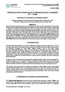
IV. Results and Discussions Figure 2 shows the time variation of the bubble volume change as a double logarithmic plot regarding the bubble growth process. The square symbols depict the experimental results at ΔTsub=10.3 K. The broken line denotes the numerical results based on original boiling and condensation model and the solid line denotes the numerical results obtained by the improved model. Here, the limitation of the bubble volume change existed because of the limitation of the computational domain size. Since the bubble growth is very fast, the experimental results in the beginning of the bubble growth process can be considered as the inertia-controlled one. It was also known as the Rayleigh equation regarding a spherical bubble growth in the homogeneous superheated liquid as follows:14) 1/ 2
⎧ 2 ⎡ T − Tsat ⎤ hlv ρ g ⎫ r (t ) = ⎨ ⎢ ∞ ⎬ t. ⎥ ⎩ 3 ⎣ Tsat ⎦ ρ l ⎭
(7)
Here, r is bubble radius, T∞ is temperature of the superheated layer, Tsat is saturation temperature and t is time. The dotted
VOL. 2, OCTOBER 2011
line in Fig. 2 denotes the Rayleigh equation. It seems that the beginning of the bubble growth process obtained by the experiment can be predicted by the Rayleigh equation. The present numerical result (the solid line) is also in good agreement with the Rayleigh equation compared to the original model (the broken line). This suggests the present boiling and condensation model may have a potential to predict the bubble growth process. Since the numerical simulations performed throughout the bubble growth process was very difficult because of the spatial- and temporal-scale changes during the bubble growth process, it requires a tremendous computational time and memory if the fix grid size (1 μm) is used for the whole computation. Therefore, in order to further progress the numerical simulations for the bubble growth process, the patch-work computations with changing the grid size are performed in this paper as follows: (1) The computation for the beginning of the bubble growth process using the finest grid size of 1 μm at first. (2) Next, the bubble volume obtained from the final result of the previous computation puts a hemisphere as the initial bubble on the larger computational domain with the grid size of 5 μm. Here, the initial temperature field is recalculated without the bubble. (3) To proceed the computation until the top of the bubble reaches to the ceiling of the computational domain. (4) The same procedure repeats on much larger computational domain with the grid size of 10 μm. On the other hand, according to the previous studies, the later stage of bubble growth process can be considered as the heat-transfer controlled bubble growth process. It was also known that the existing analytical equation proposed by Plesset and Zwick as follows:15) r (t ) = 2
3
π
Ja α l t , Ja =
(T∞ − Tsat )ρ l C pl ρ v hlv
.
(8)
Yasuo OSE et al.
Bubble volume [mm 3]
128
-1
10
10-2
(c)
10-3 -4
10
:Experiment :Rayleigh (Eq. 7) :Plesset and Zwick (Eq. 8) :Mikic et al. (Eq. 9)
(b)
Patchwork computations (Grid size=1, 5, 10 μm)
(a)
10-5 0
0.05 0.1 Time [ms]
0.15
Fig. 3 Comparison of numerical results with experimental results and existing analytical equations in bubble growth process at Tsub=10.3 K
In addition, the approximation equation containing both equations of 7 and 8 were proposed by Mikic et al. as follows:16)
[(
)
( )
]
3/ 2 3/ 2 2 + r (t ) + t t +1 − t + ,t = 2 2 , −1 , r + = 2 3 B /A B /A 1/ 2 1/ 2 ⎧ 2[T − Tsat ]hlv ρ v ⎫ ⎛ 12 2 ⎞ A=⎨ ∞ , B = Ja α (9) ⎜ ⎬ l ⎟ 3ρ l Tsat ⎝π ⎠ ⎩ ⎭
r+ =
In this paper, the numerical results by the patch-work computation are compared to the experimental results and the existing analytical equations among Rayleigh (Eq. (8)), Plesset and Zwick (Eq. (8)) and Mikic et al. (Eq. (9)) in bubble growth process. Figure 3 shows the time variation of bubble volume change as a single logarithmic plot regarding the bubble growth process. The square symbol shows the experimental results and the solid line denotes the numerical results by the patch-work computations with changing the grid size of 1, 5 and 10 μm in all directions. The dotted line denotes the Rayleigh equation (Eq. (7)), the single-dotted dashed line denotes the Plesset and Zwick equation (Eq. (8)) and the double-dotted dashed denotes the equation of Mikic et al. (Eq. (9)). In these existing analytical equations, since the influence of the degree of subcooling on the bubble growth process is appeared in the later stage because the nucleate bubble generates in the superheated layer near the wall, the temperature of superheated layer T∞ can be estimated by using the experimental results, i.e., 383 K by Eq. (7), 386 K by Eq. (8) and 393 K by Eq. (9). The summary of the comparison among them in Fig. 3 are as follows: (1) The numerical results with the grid size of 1μm for the beginning of the bubble growth process as the inertia-controlled process as shown in Fig. 3 (a) are in good agreement with the equations of Rayleigh and Mikic et al. (2) The numerical results with the grid size of 5μm as shown in Fig. 3 (b) are in good agreement with the experimental results and the equation of Mikic et al., and show a little bit apart from the Rayleigh
equation. This means that the bubble growth process is gradually changed from the inertia-controlled process to the heat-transfer controlled one. (3) The numerical results with the grid size of 10 μm as shown in Fig. 3 (c) are also in good agreement with the experimental results and the equation of Mikic et al., and are close to the Plesset and Zwick equation as the heat-transfer controlled bubble growth process. Consequently, it was found that the present boiling and condensation model can retrieve the experimental results and the existing analytical equations for both the beginning and the later stages of the bubble growth process.
V. Conclusions The numerical simulations based on the MARS with the improved boiling and condensation model based on the quasi-thermal equilibrium hypothesis were conducted for the bubble growth process. The results of numerical simulations were compared with the experimental results and the analytical equations among Rayleigh, Plesset and Zwick, and Mikic et al. As the results, the numerical results of both the beginning and the later stages of the bubble growth process were in good agreement with the experimental results and the existing analytical equations. Therefore, it is concluded that the improved boiling and condensation model with the relaxation time consideration can predict the bubble growth process of the subcooled pool boiling phenomena.
Acknowledgment This work was partly supported by a “Energy Science in the Age of Global Warming” of Global Center of Excellence (G-COE) program (J-051) of the Ministry of Education, Culture, Sports, Science and Technology of Japan. References 1) R. C. Lee, J. E. Nydahl, “Numerical calculation of bubble growth in nucleate boiling from inception through departure,” J. Heat Trans., 111, 474-479 (1989). 2) S. W. J. Welch, “Direct simulation of bubble growth,” J. Heat Trans., 41, 1655-1666 (1998). 3) G. Son, V. K. Dhir, N. Ramanujapu, “Dynamics and heat transfer associated with a single bubble during nucleate boiling on a horizontal surface,” J. Heat Trans., 121, 623-631 (1999). 4) H. Y. Yoon, S. Koshizuka, Y. Oka, “Direct calculation of bubble growth, departure, and rise in nucleate pool boiling,” Int. J. Multiphase Flow, 27, 277-298 (2001). 5) S. Shin, S. I. Abdel-Khalik, D. Juric, “Direct three-dimensional numerical simulation of nucleate boiling using the level contour reconstruction method.,” Int. J. Multiphase Flow, 31, 1231-1242 (2005). 6) G. Son, V. K. Dhir, “Numerical simulation of nucleate boiling on a horizontal surface at high heat fluxes.,” Int. J. Heat Mass Tran., 51, 2566-2582 (2008). 7) T. Kunugi, N. Saito, T. Fujita, A. Serizawa, “Direct numerical simulation of pool and forced convective flow boiling phe-
PROGRESS IN NUCLEAR SCIENCE AND TECHNOLOGY
Numerical Study on Subcooled Pool Boiling
8) 9)
10)
11)
nomena,” Proc. of the 12th Int. Heat Transfer Conf., 497-502 (2002). T. Kunugi, “MARS for multiphase calculation,” Comput. Fluid Dynam. J., 9, 563-571 (2001). V. P. Carry, Liquid Vapor Phase-Change Phenomena: An Introduction to the Thermophysics of Vaporization and Condensation Process in Heat Transfer Equipment, Taylor & Francis, 138-140 (1992). D. B. R. Kenning, Y. Yan, “Pool Boiling Heat Transfer on a Thin Plate: Features Revealed by Liquid Crystal thermography”, Int. J. Heat Mass Tran., 39, 3117-3137 (1996). N. I. Kolev, “To the Nucleate Boiling Theory,” Nucl. Eng. Des., 239, 187-192 (2009).
VOL. 2, OCTOBER 2011
129
12) I. Ohnaka, Introduction to computational analysis of heat transfer and solidification -Application to the casting processes-, Maruzen, 202 (1985), [in Japanese]. 13) Z. Kawara, T. Okoba, T. Kunugi, “Visualization of behavior of subcooled boiling bubble with high time and space resolutions,” Proc. of the 6th pacific symposium on flow visualization and image processing, 424-428 (2007). 14) L. Rayleigh, “On the pressure developed in a liquid during the collapse of a spherical cavity,” Phil. Mag., 34, 94-98 (1917). 15) M. S. Plesset, S. A. Zwick, “The growth of vapor bubbles in superheated liquids,” J. Appl. Phys., 25, 493-500 (1954). 16) B. B. Mikic, W. M. Rohsenow, P. Griffith, “On bubble growth rates,” Int. J Heat Mass Tran., 13, 657-666 (1970).