o A PARAMETER ESTIMATION ALGORITHM AND ... - CiteSeerX

"IT

o

F

DNA-TR-86-127

A PARAMETER ESTIMATION ALGORITHM AND EXTENSIVE NUMERICAL SIMULATIONS FOR THE CAP MODEL

) I

J:LL:

J.Ju, et al. University of California Department of Civil Engineering Berkeley, CA 94720

30 November 1985

Technical Report

CONTRACT No. DNA 001-84-C-0304 Approved for public release; distribution is unlimited. THIS WORK WAS SPONSORED BY THE DEFENSE NUCLEAR AGENCY UNDER RDT&E RMSS CODE B341085466 Y99QMXSC000?9 H2590D.

SEP20 1988

Prepared for Director DEFENSE NUCLEAR AGENCY Washington, DC 20305-1000

J,

%

Destroy this report when it is no longer needed. Do not return to sender. PLEASE

NOTIFY

THE DEFENSE

NUCLEAR

AGENCY

ATTN: TITL, WASHINGTON, DC 20305 1000, IF YOUR ADDRESS IS INCORRECT, IF YOU WISH IT DELETED FROM THE DISTRIBUTION LIST, OR IF THE ADDRESSEE IS NO LONGER EMPLOYED BY YOUR ORGANIZATION.

)F~

%

~

~

~

~

%

0

DISTRIBUTION LIST UPDATE This mailer is provided to enable DNA to maintain current distribution lists for reports. we would Iappreciate your providing the requested information.

SAdd the individual listed to your distribution list. El Delete the cited organization/ individual. E

Change of address.

INAME: IORGANIZATION: ___________________________

IOLD

ADDRESS

ITELEPHONE NUMBER:(

CURRENT ADDRESS

)

Z p SUBJECT AREA(s) OF INTEREST:

ZI

DNA OR OTHER GOVERNMENT CONTRACT NUMBER:

_______________

CERTIFICATION OF NEED-TO-KNOW BY GOVERNMENT SPONSOR (if other than DNA): SPONSORING ORGANIZATION:

______________________

I CONTRACTING OFFICER OR REPRESENTATIVE.:________________ SIGNATURE:_______________________________

44'

Directo

DDirector Defense Nuclear Agency TITL ~Washington, DC 20305-1000 ATTNN:

Pp.,

%%

%

%

1,4CLSSIFIED

~

~

REPORT DOCUMENTATION PAGE C

-.

a-: C C

LUCLASSIFTM IC.a :C q -" C.: ;C.S

% !-

'a

-".

"

N/A since Unclassified

3

'

-OR

-

-S-:C

'o

,E 'A, ;P< ".CS

S'R 8,

N

°

1

Approved for public release; distrbut-=

-ASS.; CA70%

:.-

unlimited.

SCv-EGA)LL

N/A since Unclassified \9R G :-GA%\ ZA7 ON REPORT %4,M8EP(S)

4

5 MONi'ORING DRGA%,ZA

2

'RORMiNG

ORGANiZATCN

60 :)F:C

7

SIMBOL

a NAME OF MONTCR%G 0a%

Director

(if 400licjel*

University of California 6c. -1ORESS Cay, Stare.

7s

A

Defense Nuclear Agency

nd ZIPCode)

7b

Department of Civil Engineering Berkeley, CA 94720

AODRESS ,City, State. ana ZIPCoe)

Washington, DC 20305-1000

Ba %ANIE o; :,140NO, SPONSORING8bO-C .. RGANVZA-:ON

VML

I

'C'EE%%%32

(if dohcEable)

SPSS/Goering

DNA 001-84-C-0304 '0 SOuRCE 09 9-r %0 NC %_%BE2S " PROGRAM 0ROjEC -ASK

0 RESS (Cry. State. and ZIP Code)

Sc.

'-VI25

DNA-TR-86-127

UCB-SESM 85/10 5a '.AME OF

0'. R;ORQ

.EMiENT NO

%O

62715H

Y99QMXS

,a

1O

,C:"SIC% 'c

C

DH008505

Include Security Clawficaton)

-

A PARAMETER ESTIMATION AIGORITHM AND EXTENSIVE NUMEICAL SIMULATIONS

OR THE CAP MODE.

'2 PERSONAL AUiJTOR(S)

Ju, Jiann-Wen; Simo, Juan C.; Pister, Karl S.; Taylor, Robert L. 3a

"0E

I3b

OF REPORT

TechnicalI

14 DATE OF REPORT

TIME COvERED

FROM 841001 "o 851031

Year Month. Day)

'5

4AC-E

851130

56

'6 S PPLS$ENr'ARY NOTATION

This work was sponsored by the Defense Nuclear Agency under RDT&E RMSS Code B341085466 Y99C.DLC00029 H2590D. COSA

:

)

09 11 '9

A8S7;ACT

CODES

02 02

\.

'

%S-GROuP_

OROP

1

SuB,ECT TERMS (Continue on reverse If neceSSary and ,onrf,

by bl4oc

numo.r

Parameter Estimation'

Colorado Concrete Data

Numerical Simulations / Cap Model

Plasticity

Continue on reverse 4 necessary And odentify by block number)

The inviscid two-invariant cap model is considered for geological materials such as concrete. A systematic constrained optimization procedure based on the Marquardt-Levenberg algorithm and the Armijo step-size rule is developed to determine values of the model parameters from available experimental data. The predictive capabilities of the cap model and the efficiency of the parameter estimation procedure are assessed through extensive numerical sirulations based on well-documnted experimental concrete data from the University of California. 7% ,.

0 3,STRIBUTION AIAILABLITY OF ABSTRACT r-INCLASSIFIEO,,NLMITED M SAME AS RT

21

,

'.

83 APR edition may O .s1. uftI exnausted aSust s are obsolete

i

,,w.'.

22c OFF'CE SYMBOL

DNA/CSTI *EC*.,ITY CLSaSSIoC4_AON OP

-

UNCIASSIFIED

,.

•

Nr

,?

ASTRACT SECRITY C.,ASSiFCATION

(202) 325-7042 ai All OtM~f #otr


0,

0

(4)

I.

(

2

'r C

.

L.0

,1

2a D ICORNER

Tj 2~

--SINGULAR REGION

Y

Fe

-D S.,.

ELASTIC REGION

"

0

L(K)

X()

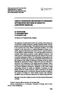
Figure 1. The yield surface for cap model. F, and F c denote the failure envelope and the hardening cap surface, respectively. The shaded area is the "singular comner region". 5.

1(a

0

tSV(X) a W

(I

exp [-D

-

X(x)J

(5)

"Mr

where X(E) is defined by X(K)

In the above expressions,

a,

=K

+

R Fe(x)

(6)

0, -y,E),W , D , and R are material parameters which characterize

the two-invariant cap model considered here.

I P-'.

4S

Ir AF

%

%

%

.etk %

%

%

d-Mh-

e~~~~

%

%.

-PiM.

SECTION 3 PARAMETER ESTIMATION AND NUMERICAL SIMULATIONS In order to assess the capability of the two-invariant cap model in predicting response behavior for actual materials such as concrete and geomaterials, model parameters need to be estimated from available experimental data. In this section, a parameter estimation procedure and an assessment of the predictive capability of the cap model are presented. This is followed by extensive numerical simulations for the Colorado concrete data.

3.1. PARAMETER ESTIMATION.

MARQUARDT-LEVENBERG

ALGORITHM.

It is characteristic of currently employed parameter estimation procedures for the cap model (see e.g. [5,6]) to fit separately the failure envelope, cap surface, and hardening law parameters. Typically, asymptotic failure points from TE, TC, SS, CTC, CTE, RTE, RTC and PLt arc used with a Icast-square fit procedure to estimate the failure parameters; whereas

-0

iso-plastic volumetric strain contours are employed to estimate the cap shape parameter R.

,, ,

The hardening law parameters D and 4" are determined from HC tests4t Although this pro-

,-

cedure provides a parameter fitting directly associated with the physical construction of the

-41

cap model, it has the following two major drawbacks: (a) a large amount (more than 20 tests) of conventional experimental data are required (e.g. CTC, CTE etc.), and (b) it is not possible to utilize some existing nonconventional experimental work: e.g., the results from the "Colorado" experimental program [4]. Hence, a more flexible and systematic parameter estimation procedure is needed. This is the objective of the following section. Optimization algorithm The basic idea of the procedure advocated here is to regard the optimal fitting process for given experimental data as a least-square constrained optimization problem.

In this context, the objecti'e function II: R -R

is simply the sum-of-squares

error function defined as I1 =E A

art(41,,, E

- 0,;11

(7).

%vicrc V • nmber of'ohs'ervation. t I L sltadt 1or rixial .'xtensioni. I tria xial compreNsion. SS simplc %hiar,(.TC conventional triaxial compression. CTE con..nnonal triaial cxtLenson. RTE reduced triaxial extension. RTC rcduced iriaxial cornpression. and PL proporional loading. H ( represents hdrostaic conprcssion Ist.

% 6%

.

I,3/ "'/ '',, d'Ae'_'%,e"e ,. .', ,.'),;

e,..e',.,, V

,e,,"%eir~e.ei.'.-e,')ee

~o,

,. *-,".'qe ,.S,.",-,

el:

stress response from constitutive model considered

,r;: observed stress response

*: parameter vector (in R' for cap model) I:

ph data point

In the following, this procedure will be illustrated using the cap model. It is, however, generally applicable to any constitutive model. The constraints imposed on the optimization problem emanate from physical restrictions placed on the cap parameters. For example, for a one

model

meaningful

physically

a>0,">0,a>-,0>0,0 R >0, D >0, W>0.

These

should constraints

define

r

P-.

have a feasible

-.

7

0

domain --CR , which is a convex polygon. The resulting constrained optimization problem is then expressed as min II(*t)

Find:

subject to

*e

(8)

There exists a wide variety of algorithms for solving the standard convex optimization problem (8) (e.g., see [9] for a review). The algorithm employed here is the well-known Marquardt-Levenbergalgorithm together with the Armijo step-size rule [7-10]. This algorithm is essentially a hybrid of Newton and steepest descent (gradient) methods. It combines the ability of the steepest descent method to converge from an initial guess, which may be outside

,

-

the region of convergence of other methods, with the asymptotic quadratic convergence characteristics of Newton's method near the solution. The Marquardt-Levenberg algorithm can be summarized in the following form: *,i

I= i*

(9)

+ Xi hi -

hi = -[H, + 7/D] Hi - 2 Qr Q,

Qi = 17,

(10)

' Viri

(approx. Hessian) (sensitivity matrix) 0*,

(11) (12)

0

= Marquardt parameter

D,= liagonal matri\"of 1l, or Vimpl" I X,

I

a

r K m

.Il

,i,

il

l

'

W4 ,

C,,--.

lI(*l .1) < [1(*,i )}

(13)

. 0

,IWP,1

lI''

For problems where Q, may not be easily constructed analytically the derivatives are typically computed by means of forward differences. However, central differences provide greater

6

.r

1%-'" S

6.

accuracy in the vicinity of the solution (minimum); thus, central rather than forward differences are employed in computing Q, when the solution is closely approached. In addition, to minimize the number of function evaluations (stress responses), a rank one update to the sensitivity matrix is used periodically (similar to the Quasi-Newton method)

I I112[ ((, - 1)- (*,) - Q, Q, + 11 l'*',.

Q,.1 where A*,,,

- ,,..+ -

,.

(14)

In Eq. (10), for a given value of 1,,

Cholesky factorization of

H, + 77,D, is employed to check for positive definiteness. If the factorization breaks down, i.e. H, + 1,D, is not positive definite, then 77,is increased. The algorithm summarized above can be systematically applied to any set of experimental data to obtain the optimal fit for the constitutive model under consideration in a least square sense. Error measurement During the optimization process, a root-mean-square (RMS) type of error measurement is adopted. The optimization process is considered to reach its optimum when the RMS measure is minimized. The relevant measures are defined as follows:

•

_-

N 6

J

M%

(15)

(RMS of error)

A' a-- -

(RMS of observed responses) NS

(16)

(normalized relative RAMS error)

(17)

Remark 3.1. It is interesting to examine the sensitivity of the response under perturbations in cap model parameters. A finite difference sensitivity matrix Q is defined in dimen-

0

sionless form:

Q'i where a, is a stress component (i

A r,- / a1

- . .

(18)

=

1,...,6) and ,I'j is a parameter component (j

=

=

I.7),

0

respectively. A standard sensitivity analysis reveals that the response of the cap model is relatively insensitive to changes in the model parameters.

By ordering the model parameters

according to relative sensitivity in the response, one obtains in decreasing order of sensitivity: Wl--, D

R -,

-.- 09

) .

(19)

In summary, one obtains the following relative degree of sensitivity (from large to small): h/ rd(',litv palr(IItt('l('ra

-

(J,1l

.'e

rale('(r%-=" Illdur' )a(lrtl('fer " 0"

7% L

,,

¢r

"

'

i'',O_ , ,_2v _ ,.r,.

' _,.

,.= 4_..a.

._

,_,_..,,...'-'_.i.'.'-'.,.,'..-..

.,.

3.2. PREDICTIVE CAPABILITIES. "COLORADO" CONCRETE DATA. In this section, we first examine the consistency of the 'Colorado concrete* data [41, next we estimate the model parameters by exercising the procedure described above, finally we assess the predictive capability of the inviscid cap model. Colorad concrete data. This experimental program on concrete was performed at the University of Colorado (1983) and is well-documented [4]. The program consists of six major series of nonconventional multiaxial stress-strain curves. The total number of experiments is 67. The data are characterized by the following properties: (a) characteristic uniaxial compressive strength f, = 4 ksi, (b) mean pressure < 8 ksi (c) truly triaxial states of stress for concrete, (d) nonconventional complicated stress paths, and (e) quasi-static loading. The six major series of tests consist of the following: (1) A series of 12 cyclic triaxial tests, consisting of cyclic hydrostatic preloading to various stress levels, followed by proportional deviatoric stress cycles without reversal along triaxial compression, simple shear, and triaxial extension paths. (2)

A series of 8 cyclic triaxial tests, consisting of cyclic hydrostatic preloading to various stress levels, followed by proportional deviatoric stress cycles with reversal along the same deviatoric paths as in Series 1.

(3)

A series of 17 tests consisting of hydrostatic loading, followed by proportional stress

(4)

deviation, followed by a circular stress path within the deviatoric plane. A series of 22 axisymmetric triaxial tests to explore load path effects. In addition to pro-

. •

portional and hydrostatic-deviatoric paths, this series contained staircase-type loadings to explore convergence to the proportional path, tests with hydrostatic stress increments (5)

with and without hydrostatic preloading, and tests under non-proportional loadings. A series of 6 tests within the deviatoric plane, as well as a number of other tests

S

specifically designed to check the meaning of loading and unloading. (6)

A series of 2 tests of piecewise-uniaxial loadings.

P

Assessment of data consistency. Basically, the measures employed here are the same as those discussed in the previous section. For convenience, these measures are summarized as follows:

ri~uv1 N j

(see( 15))

(20) ., . .6!..

2

u~''''h [N

ICAIII'

TN

(see(16))

(21)

N

I'

(.VLM 17 ))

(22)

8 p, N1Vi"

8

",

Here e' refers to a strain measurement of test 'A'. An assessment of consistency for the "Colorado' concrete data may be obtained from the replicates of experiments available in the reported results [4]. The present analysis generally indicates reasonable consistency of the data. However, some serious discrepancies between replicates are also observed. See Table I below. Table 1. Consistency of the Colorado concrete data [4].

Tests

6%

Major Path

1-1 & 1-10 1-4 & 1-7

13.5 31.1

CTC TC

1-6 & 1-9

51.3

TE

2-3 & 2-4

9.6

SS

2-7 & 2-8

13.5

SS

3-1 & 3-2 3-3 & 3-4

244.3 47.2

Circular

3-10 & 3-11

92.9

Circular

4-1 & 4-2

10.9

Axisymmetric

4-6 & 4-7

54.2

Circular

j

Axisymmetric

Model parameter estimation procedure. The actual data employed in the optimization process based on the Marquardt-Levenberg algorithm are obtained by arbitrarily selecting one test out of each of the six major series. Thus, a total number of 6 tests is used in the actual fit of the model. The quality of the fitting is satisfactory. Typical values of the RMS error

0

found from back-prediction using the optimal material properties are: 6 - 16% for test I-I (CTC), S= 8.5% for test 2-3 (SS), 6 = 26% for test 3-11 (circular), 6 = 11.5% for test 4-11

lel

(axisym.), etc.. From this optimization procedure, we obtain the following set of parameters which best fits the observed experiments: a = 3.86ksi, 0 =.11, -y=1.16ksi, #=.44ksi - , R =4.43, D=.0032ksi' , W=.42, X 0 =16ksi. Predictive capability. After the optimal model parameters are obtained, the resulting cap model is used to predict the response of every other Colorado test which is not included in the optimization process (total number = 61). It is emphasized that the "prediction* here has nothing to do with optimal fitting, but is obtained by exercising the cap model using previously estimated parameters.

In general. considering the experimental data scatter, the

predicted response is in good agreement with the experimental results. It is noted that the ,,Wrall qualtiative behavior for the Colorado concrete data is captured. Values of the RMS error corresponding to a selected sample of simulations are summarized in Table 2 below. 9

vI

;-;. +.;. .-; +,;-;;. ,.,,:-',:%,;% :..;,.--.;-4'= ,.:..:;--.. .s....". ..'.";.. --

---

-P

--

--

-

-

...

N.5'._ '-

: ..:..." ...;,:. :..-.. ..-...... :....-.. . ..

.

.

.

.

. .

. ..

'

+

The overall RMS and standard deviation of error for 61 tests are 26.6% and 14%, respectively. A comparison between experimental and predicted stress-strain curves is contained in Figures 2-I1.

0 Table 2. Results of prediction. Inviscid case

Tests

6%

Major Path

1-2

12.4

SS

1-3

14.1

TE

2-2

17.

TE

2-4

11.7

SS

3-5

15.

Circular

3-17

11.6

Circular

4-7

14.

Axisymmetric

4-12

11.4

Axisymmetric

5-1

14.

Unsymmetric

5-2

17.

Unsymmetric

'--,

Assessment and evaluation. From the above fitting and prediction exercises, it may be concluded that the inviscid cap model generally exhibits good fitting and predictive capabili-

.

ties for the Colorado concrete data. The simulations reported herein capture the overall qualitative behavior of the experimental response.

,..

0

-p,.., 10?

.- A%

- r NV'

NII,'. %

LI)I ,l-

UU"L

r

LL

'..

o

Sl

ru 0

Cl --

=

".

t- I w.-

xI'

w

a))

'

M-

)

0 CL~U

c

0r

W

Cu

%u IF.IW e . LU%

r "a ". %

.'

0

I-x

x

0U

-#> u

oUCU.=

(U C,6

cu

X

C)4 -.-.

-

0

U)m

I

)

E

C

-

c 0

U;-4

0

JWo

ti)LX"Z rx W(n.(

-

0

(UU

0

F_

o

N~ V

w

0

0

Z; a 0 LL

v

p0 J0

x~

0X

IL

w

0

U)

0l

4 0-

0

Id U

0

0

0n u0U)0

LAm0D :

a

tU)

-

1320-

0% 0~

w

%

0

%

%

p

N

N

uCu

o

cu

L) 41*

0

%V

0 *n

u-

0 0

'C-

1

(1)

a.. C)

w

C-4.

U. 0

m-

00

17)co r

m

o

c

no LQ

Z: 0 required 20 if (para( 1).le.0dO) then go to 30 c para(3) > 0 required elseif (para(3).le.0.dO) then go to 30 c para(3) < para(1) required elseif (para(3).gt.para(l)) then go to 30 c para(3) > 0.1 *para(l ) preferred elseif (para(3).It.0. I*pa.rj( )) then go to 30 C para(2) > 0 requircd elseif (para(2).It.0.dO) then% go to 30 c para(4) >= 0.21 preferred elseif (para(4).It.0.21Id) then go to 30 C para(4) < = 2 preferrcd ciscif (para(4).gt.2.OdO) then goto 30 C para(5) > = 1.6 preferrcd elscif (para(5).lt.1I.6d0) thien go to 30 C para(6) and para( 7 ) > 0 required cleta.(para(6).Ic.0.dO.or.para( 7).le.0.dO) thiei go to 30

r,

.

*r

~~A

26

%

%q

else if O.K. go to 50 endif c.... Half the increments for parameters if constraints are violated.N 30 do 40i=l1,7 delp(i)=delp(i)/2. 40 para(i)=old(i)+delp(i) go to 20 c.... Update the old parameters 50 do 60 i - ,7 60 old(i)=para(i)

c

61 62 63

64

65

70

do 70 j=l1,6 if (indi.eq.l1) go to 63 do 62 k= l,noj) do 61 kk=l1,6 deltem(k,kk) - del(k,kkj) continue continue call main(ytemp,noj),para,deltemij,indi) do 65 k=lI,noj) y(kj) = ytemp(k) ytemp(k)= 0.0 do 64 kk=l1,6 del(k,kkj) - deltem(k,kk) deltem(k,kk) =0.0 continue continue continue indi=indi+ I

c knt-0 do 200 j -1,6 do 100 i -l,noj) k=knt+i 100 continue knt-knt+noj) 200 continue return end

27A V0 %1

!!Zt

%%

subroutine main(y,n,para,del,ino,ind) c.... DEL :the specified strain increment vectors. implicit double precision(a-h,o-z)

common/state/sig0(6) common/sta/geop,xint c.... Y : the response vector c.... PARA : the parameter vector dimension del(500,6),sig(6) dimension y( l),para(1) common/fix/bulkm,shearm,zm c.... Material parameters : common/prop/Itype,tcut,fcut common/elas/bulk,shear common/par I/alpha,theta,gama,beta,r common/par2/d,w,z c.... Definition for parameters (just for convenience). bulk=bulkm shear= shearm alpha=para() theta=para(2) gama=para(3) beta= para(4) r=para(5) d=para(6) w=para(7) z=zm c.... IND flag, f .,d= 1 , read strain increment data c.... INO: identifier for test # ino ( 1-6). if(ind.ne. 1)go to 200 iftino.ne. 1) go to 50 c.... Read common input data: ltype,tcut,sig0,geop,xint c.... Read material type and tension cutoff criterion c.... TCUT is in terms of live stresses. read(5,*) Itype,tcut

c.... Input the initial states of stress and strain read(5,O) (sig0(k),k= 1,6) c.... Input the geostatic pressure and XINT( the initial cap) read(5,*) geop,xint c.... Strain controlled CAP model c.... Read input data del and initial strain. 50 do 100 i=l,n read(5,*) (del(i,k),k= 1,6) 100 continue c.... Call preprocessor INITEL to calculate elint from c given xint and fcut(in total stress) c.... XINT := the inital X value for the initail cap. c.... Z := the X value for the characteristic initial cap. c i.e. the X value when EVP = 0. 200 if(ino.ne.l) go to 210 call initel(xint,elint,nocon l,nocon2) c.... Assign initial state of stress and strain accordingly c

-8

x

0

210

continue do 220 k= 1,6 sig(k)=sigO(k) 220 continue el =elint c.... Call 3-D strain history driver call drv3D(n,y,del,el,sig) return end

0

S 29

S .4"

I

c subroutine drv3D(n,y,del.el,sig) c

c..This routine is a 3-D strain history driver and the variable increments are deps stored in array del. implicit double precision(a-h,o-z) cornmon/sta/geop dimension del( 500,6),sig(lI),deps(6),y( I) comnion/prop/ltype,tcut,fcut common/elas/bulk,shear common/par I/alpha,theta,gama,beta,r commonlpar2/d,w,z

c do 200 i=lI,n do 100 k- 1,6 deps(k)-=del(i,k) continue 100 call cap(sig,deps,geop,el,mtype,it,nocon,sj I ,sj 2,xl,evpi ,ejl,ej2d,flej 1) y(i)-sig(3) 200 continue% return end

30

e

piE'

%

%

subroutine cap(sig,deps,geopel,mtypeit.nocon,sj l,sj2,

xl.evpi,ej I .ej2dfl ej 1) For full three-dimensional stresses and strains c.... computations by using the CAP model c Strain controlled algorithm. c .... Stresses and strains are sig and eps, respectively. c.... geop = geostatic pressure (overburden stress) c.... c.... el = hardening parameter mtype : 0 - tension cutoff, I = elastic. 2 = failure, c.... 4= cone mode 3 = cap mode. c.... it - # of iterations for CAP mode calculation c.... nocon = I indicates no convergence under max iterations c.... (nit) restriction. Otherwise = 0 c.... eps - error tolerance parameter c.... Itype : I soil, 2 = rock c.... implicit double precision(a-h,o-z) common/prop/ltype,tcut,fcut common/elas/bulk,shear common/par l/alpha,theta,gama,beta,r common/par2/d,w,z dimension sig(l ),deps( I ),s(6),de(6)

S

9

data eps/ l.d-6/ Statement function for exponential with negatively large c....

argument for large caps c .... exps(z)=dexp(dmax I (-500.,z))

Failure envelope function for sj2 c.... fI (sj 1)=alpha-gama*exps(-beta*sj l)+theta*sj I d l (sj 1)= theta+ gamambetaexps(-beta*sj 1) Cap statement functions for f2 functional forms c.... capl-l(k) :intersection point of fl & f2, c.... x(k) :intersection of f2 & j 1 axis c.... capl(el)=dmax 1(0.O,el) ra(capi)=r x(el)=dmax l(0.,el+ra(capl(el))*fl (el)) evp(xl)=w*( I.0-exps(d*(z-xl))) f2(sj I ,xl,capi)=dsqrt((xl-capi)"2-(sj 1-capi)**2) " /ra(capi) Elastic moduli functions c.... bmod(sj l,ev) -bulk smod(sj2,ev)-shear

c it=0 nocon=O dev=deps( l)+deps(2)+deps(3) devb3 =dev/3.0 do I k-l,3 I de(k)=deps(k)-devb3 do 2 k-4,6 2 de(k)-deps(k) press-(sig(l )+sig(2) +sig(3))/3.0 do 3 k- 1,3 3 s(k)=sig(k)-press

31 W.Vr W

,.

.,

,,."

B

do 4 k=4,6 4 s(k)=sig(k) sj lt= 3.*(press+geop) temp =0. do I1I k=l13 II temp=temp+0.5s(k)*s(k) do 12 k=4,6 12 temp=temp+s(k)*s(k) sj2l =dsqrt(temp) capi ~capt(el) X1= X(cl) evpi =evp(xi) c.... Elastic material properties threek= 3.*bmod(sjlIt,evpi) g=smod(sj2l,evpi) twog =2. *g c.... Elatic trial sj I= threek*dev +sj It do 13 k=I1,6 13 s(k)=s(k)+twog*de(k) ratio= 1.0 mtype = 1 c.... Tension limit test tencut=dmax l(fcut,tcut+3.*geop) if(sjlI.gt.tencut) go to 10 sj I=tencut ratio=0.0 sj2=0. mtype=0 c If no contraction if(ltype.eq.2.or.el.e.0.OdO) go to 200 c .... Tension dilatancy coding for soils with el.ge.0.0 c.... Dilatancy controlled by contracting cap up to eI.ge.0.0 ell=dmin I(0.0,el-eps*fl (el)) xll =x(ell) denom =evp(xll)-evpi if(denom.1t.0.OdO) go to 5% el =0.0 go to 200 5 devp=dev-(sj l-sj lt)/threek denom=dmin l(denom,devp) el=el+devp*(ell-el)/denom0 el=dmaxl(0.0,el) go to 200 c.... Check if failure envelope mode is invoked 10 continue temp=0. do 14 k=l1,3 14 temp-temp+0.5s(k)*s(k) do 15 k=4,6 15 temp-temp+s(k)*s(k) sj2=dsqrt(temp)

32

.'

%\N

__

III

j1N~xn~xn VVIVIINr K 97%MF

If cap mode if(sj l.gt.capi) go to 40 ej2d =sj 2 c.... TMISES is the sj2 value at the corner point(tmises>=-fjl1) tmises f2(capi,xl,capi) c

ej I -Si

Il-fl(sj 1) fi ej I= fj 1 fe=sj2-dmin 1(fjlI,tmises)

c I elastic

iqfe.le.0.0d0) go to 200 c.... If kO =0: c If JIE=L(kO), J I=L(kO)=J IE. k=kO elseif (dabs(sj I-capi).le. Ld-6) then mtype=4 go to 30 endif c.... Failure envelope surface calculation ( fl mtype=2 elold=el c.... Iterate to find new k & J31 call proj(deps,el,sj I,2,sj 2,nocon,it,threek,g) c.... Consistency check for cap model: if(ltype.eq.2.or.elold.eq.0.dO) el=elold if(sjlI gt.el) el -sjlI if (Itype.eq. I .and.elold.gt.0.OdO) then iftdabs(el-sj I ).le. 1 d-6) mtype=4 el = max(el,0.OdO) endif el = max(el,0.OdO) 30 fjl=fl(sjl) sj2 =dmin 1(fil ,tmises) ratio =sj2/sj2e go to 200 c.... CAP mode calculation 40 iftsj I.gt.xl) go to 50 c If elastic if~sj2.le.f2(sj I ,xl,capi)) go to 200 S0 mtype= 3 call proj(deps,el,sj I ,3,sj2,nocon,it,threek,g) ratio=0.0 iftsj2e.ne.0.OdO) ratio-sj2/sj2e 200 continue c.... Update dev. stresses do 300 k=l1,6 300 s(k)=s(k)*ratio press =sj I/3.-geo p c.... Caic. live stresses do 400 k= 13

33I

sig(k)-s(k)+press do 410 k=4,6 410 sig(k)=s(k) c.... caic. X and vol. plastic strain .0 xl=x(el) evpi =evp(xl) return end c subroutine proj(deps,el,sj I ,mtype,sj 2,nocon,it,threek,g) 400

C

****************************

c.... Subprogram to calc. the k and JI iteratively by modified c

Regula Falsi Secant Method. implicit double precision(a-h,o-z) common/prop/ltype,tcut,fcut commonfelas/bulk,shear common/parlI/alpha,theta,gama,beta,r commonlpar2fd~w,z dimension deps( I) data nit/600/ data eps/ 1.d-6/ c .... Statement function for exponential with negatively large c.... argument for large caps exps(z) =dexp(dmax I(-500.,z)) c .... Failure envelope function for sj2 f I (Si I)=alp ha-gamaexps(-betasj 1)+ thetasj I dlI (sj 1)=theta+ gamabetaexps(-betasj 1) c .... Cap statement functions for f2 functional forms c.... cap]l=J(k) : intersection point of f) & f2, c.... x(k) :intersection of f2 & j I axis capl(el) =dmax 1(O.0,el) ra(capi)= r x(el) =dmax I(0.,el +sra(capl(el))*flI (el))A evp(xl) = w( I .0-exps(d*(z-xl))) f2(sj I ,xl,capi) =dsqrt((xl-capi)*(xl-capi)-(s Il-capi)*(sj I1-capi)) "/ra(capi) d2(sjl1,xl,capi) =-(sjlI capi)/ra(capi)/dsqrt((xl-capi)**2c....

0

0

Elastic moduli functions bmod(sj I ,ev) =bulk smod(sj2,ev) = shear 0 nocon=0 it=O sj Ice= s I si 2e = Si2

xl =x(el) evpi =evp(xl) c .... Convergence criterion conv =eps*0. 1 c .... Failure mode c Initial guess if (mtype.eq.2) then

34

m,

-0

*A

l

Srw

elI~sj le elr=eI else go to 45 endif c.... tcut >

-I

xll=x(ell) devpl =evp(xlI)-evpi sj II= sj Ile-threekdevpl ql =-(sjll + 1.)I(sj Ie+ 1.) C

xlr=xl devpr=evp(xlr)-evpi Si 1r= sj Ie-threek*devpr qr=(xlr-sj 1r)/(xlr-j Ie) go to 47 c.... Cap mode0 45 ell=eI elr- sj 1Ie if(sj le.ge.xl) ql=(ei-sj le)/(eI-xl) ifqsj Ie.lt.xi) qi =2.*sj2e/(sj2e+ f2(sjl1e,xl,capi))- 1.0 xr= x(elr) sj lr=sj le-threek*(evp(xr)-evpi) qr=(xr-sj Ir)/(elr-xr) 47 qold=O.0 c.... Modified Regula Falsi Method do 80 it- I,nit, c Secant method el =(qr*e!I-ql*elr)/(qr-q1) xl=x(el) devp= evp(xl)-evpi sj I =sj Ie-threek*devp capi =capl(el) if~mtype.eq.3) go to 48 c If Failure mode c el >=-I if(sj I.gt.el) qc=-(sj I+ I .)/(el+ 1.) if(sl.le.sjle) qc=(xi-sjl)/(xl-si le) if(sj I .gt.eI.or.sj 1.1e.sj Ie) go to 60 sj2=fI(sjl) go to 49 c If Cap mode 48 continue% if(sj I.ge.xl) qc=(eI-sj l)/(eI-xl)% if(sj 1.le.capi) qc=(xI-sj 1)/(capi-xl) if(sj 1.ge.xI.or.sj I .1e.capi) go to 60 sj2-f2(sj I ,xl,capi) 49 if (mtype.eq.2) then0 c** If cone mode (at corner pt.) inside failure mode*** if~dabs(el-sj I ).Ie. I d-6) then c.... Correct treatment slope= (sj I-sj Ie)/(sj2e-s2)g/(3.*threck) desp devpl( 3.*slope) else

0 ..

10

*

,

-

%

35

N., %

%..

s'%

desp=devP/(3.*dI (sj )

endif else desp=devp/( 3.*d2(sj I ,xl,capi)) endif a=sj2-g*desp error= si2e-a qc=error/(sj2e+a) c.... Convergence criteria if(dabs(error).le.conv) go to 90 60 if(qc.gt0.OdO) go to 70 if (mtype.eq.3) then c k too large elr=el

c

'

qr=qc ifqqold.lt.0.0d0) ql=0.5*q1 else k too small ell-el ql=qc if~qold.1t.0.OdO) qr=.5*qr endif go to 80

c 70 if (mtype.eq.3) then k too small elI=el ql=qc if~qold.gt.0.OdO) qr=0.5*qr else c k too large elr-el qr=qc iftqold.gt.0.OdO) ql=0.5*ql endif 80 qold-qc c c.... If no convergence within NIT iterations: nocon- I% c If cap mode: if (mtype.eq.3) then sjtI =dmin I(sj I ,xl) if(sj I .lt.capl(elr)) sj I =capi sj2=dmin l(sj2e,f2(sjlI,xl,capi)) c If failure envelope mode: else Si I =dmin l(sj I ,el) endif c c 89 continue 90 return end C subroutine initel(xint,elint,nocon I ,nocon2) c

36

0

c0

c value of el(hardening parameter) for a given c initial x(el) value. c.... Also, it solves FCUT,the intersection of Fl and0 c

JI-axis.

implicit double precision(a-h,o-z) common/prop/ltype,tcut,fcut common/elas/bulk,shear common/par I/alpha,theta~gama,beta.r common/par2/d,w,z data eps,nit/ I.d-6,60/ c.... Statement function for exponential with negatively c large argument for large caps exps(z)=dexp(dmax 1(-500.,z)) c.... Failure envelope function for sj2 flI (sj I)= alpha-gama*exps(-beta*sj 1)ithetasj I c.... Cap statement functions capl(el)=dmax 1(O.O,el) ra(capi) =r x(el) -el +ra(capl(el))*flI (el) c.... Elastic modulus function bmod(sj I ,ev)= bulk c .... Find initial el c Solve ftk)=x(k)-xint=0 , not related to Z. c .... xint is reset so that within the convergence criteria c xint is positive ( because we assume x>0, i(k)>=O.) c .... noconI=I means no convergence for initial el iteration nocon2 = I means no convergence for fcut iteration c c xint=dmaxlI(xint,eps*0.000l *bmod(0.,0.)) c.... Make initial guess kO e10=xint*0. I fi =x(elO)-xint c.... Make second initial guess k I el I =(xint-0. 1*dmax. I(dabs(xint),fl1(xint)))*0.05 c .... Set up convergence criterion conv=dmin I1(1 d-7,xint) c .... Secant iteration do 100 it=lI,nit fl I = x(ellI)-xint if(dabs(fli).lt.conv.or.dabs(ell-elO).lt.conv) go to 200 e12 = el I-fl 1O(eI I-elO)/(fl I-fib) elO=ell el I =e12 100 continue noconlI = I 200 elint=ell c.... Find fcut c Solve fl(fcut)=0 c.... Make first initial guess for fcut fcut=dmin l(0.,elint) del -f I(fcut)

e

37

if(deleq.0.dO) go to 600 c.... Make two better initial guesses for fcut do 300 it- l,nit dO = fcut-del flO= fi(elO) if(flO.It.0.dO) go to 400 del= Il0.*del fcut-.elO 300

1

~'m

continue

c.... Secant iterations 400 do 500 it=lI,nit fl I=fI(fcut) ifodabs(fl I).lt.conv.or.dabs(fcut-eO).It.conv) go to 600 e12 -fcut-fl I*(fcut-elO)/(fl 14-fi) eIO=fcut flO=fll fcut =e12 500 continue nocon2= I 600 return end

Ir.I

%

%a

381

?.X~~~a

I%

X

Aru

.

%~~~~

%

subroutine dprint(y,n I,n2,name) c.... Program for printing response y (sig-33). implicit double precision(a-h,o-z)

h.

dimension y(l) character*6 name

4.

write(6,2000) name c .... Print out 8 columns each time.

do 100 j-nl.n2,8 c .... JH : the right-most index. jh=j+7 if(jh.gt.n2) jh=n2 write(6,2001) (n,n=jjh) write(6,2002) (y(k),k=jjh) 100 continue return c.... Format 2000 format(////20x,a6/

* 20x,' ..... ==

2001 2002

W,

)

•

format(//8x,8il 5) format(/8x,8d15. 7 ) end

391

0, It.%%"1

1W

APPENDIX B EXAMPLE INPUT AND OUTPUT FOR APPENDIX A

INPUT BULK MODULUS, SHEAR MODULUS, AND INITIAL CAP (Z) PARAMETER: 2100. 1700. 0. INPUT NO. OF OBSERVATIONS FOR 6 TESTS: 47 49 45 48 49 48 INPUT OBSERVED (EXPERIMENTAL) STRESS RESPONSES FOR 6 TESTS: NO.1 5. 6. 5. 4. 3. I. I. 3. 8. 9. 10. 8.8 9. 8.8 8.6 8.3 II. 10.5 9. 8. 10. 12. 13. 12. 14. 14.9 13. 8. 10. 12. 10. NO. 2 4. 6. 8. 8.5 9. 9.5 1. 2. 8. 7.5 7. 6.5 7. 7.5 9. 8.5 9. 9.5 10. 9.5 9. 8.5 8. 8.5 7.5 8. 7.5 7. 6.5 6. 6.5 7. 10.5 10. 9. 8. 8. 9. 10. 11. 7. 6. 5. 4.5 4. 3.5 3. 2.5 2. NO. 3 10.09 6. 8. 10. 10.12 1. 2. 4. 9.06 8.73 8.37 8. 9.99 9.84 9.625 9.36 6. 5.91 7.63 7.275 6.94 6.63 6.375 6.16 6. 6.16 6.375 6.63 6.94 7.275 5.89 5.91 9.36 9.625 9.84 7.63 8. 8.37 8.73 9.06 8. 9.99 10.09 10.12 10. NO. 4 7. 8. 1. 2. 3. 4. 5. 6. 10.122 10.828 11.536 12.246 12.95 13.656 8.708 9.414 7.823 7.646 7.293 6.939 12.246 10.828 9.414 8. 8. 8. 8. 7.293 7.646 8. 8. 8. 8. 8. 8. 8. 8. 8. 8. 8. 4.466 8. 7.823 7.646 8. 7.292 6.584 5,172 NO. 5 5.698 1.5 2. 3. 4. 4.566 5.132 1. 5.414 4. 3.717 3.434 3.151 2.869 6.262 6.828 2.586 2.586 3.293 4. 3.717 3.434 3.151 2.869 7. 7.5 8. 9. 3.293 4. 5. 6. 6.828 6. 4. 4.708 5.414 6.122 10. 8. 6.828 6.828 6.828 6.828 6.828 6.828 6.828 6.828 6.828 NO. 6 1.56 .88 0. 0. 3.6 3.6 2.92 2.24 0. 0. 0. 0. 0. 0. 0. 0. 1.56 2.24 2.92 3.6 3.6 3.6 0. .88 1.56 .88 0. 3.6 3.6 3.6 2.92 2.24 3.6 4. 5. 6. I. 1.5 2. 3. INPUT CONVERGENCE CRITERION AND MAXIMUM NO. OF FUNCTION EVALUATIONS: 5 !.d-I1 0.000001 500 2 INPUT PARAMETERS FOR MARQUARDT-LEVENBERG ALGORITHM:

41

0

0

INPUT INITIAL GUESS FOR MATERIAL PARAMETERS: 3.2 .09 1.0 .49 4. 0.004 0.2 INPUT OPTION FOR WEIGHTING MATRIX (0: WEIGHT = IDENTITY): 0 INPUT OPTION FOR SOIL (1) OR ROCK (2); AS 1 -0.3 INPUT INITIAL STRESS STATE: 0. 0. 0. 0. 0. 0. INPUT GEOSTATIC OVERBURDEN PRESSURE 0. 16. INPUT STRAIN HISTORY OF 6 TESTS: NO. 1 -0.0000020 -0.0000587 -0.0000635 0. 0. 0.0002395 0.0002086 0.0001715 0. 0. 0. 0.0004127 0.0004370 0.0004799 0. 0. 0.0003060 0.0003555 0.0003940 0. -0.0001604 -0.0002206 -0.0001891 0. 0. -0.0003913 -0.0003993 -0.0003953 0. 0. -0.0001187 -0.0001047 -0.0001095 0. 0. -0.0000720 -0.0000330 -0.0000827 0. 0. 0.0001420 0.0000992 0.0000880 0. 0. 0.0004722 0.0004828 0.0004767 0. 0. 0.0005390 0.0006185 0.0006685 0. 0. 0.0004835 0.0005567 0.0005853 0. 0. -0.0001502 -0.0002710 -0.0001843 0. 0. -0.0001722 -0.0002279 -0.0002293 0. 0. -0.0001348 -0.0001654 -0.0001603 0. 0. -0.0004710 -0.0004949 -0.0005204 0. 0. -0.0001411 -0.0001104 -0.0001218 0. 0. -0.0001776 -0.0001480 -0.0002248 0. 0. 0.0004733 0.0004259 0.0004466 0. 0. 0.0004973 0.0005316 0.0005792 0. 0. 0.0004338 0.0005852 0.0005394 0. 0. 0.0011258 0.0011877 0.0012631 0. 0. 0.0000354 -0.0000029 0.0003382 0. 0. 0.0000676 0.0000314 0.0002335 0. 0. -0.0000763 -0.0000882 0.0001768 0. 0. 0. 0. 0.0000006 -0.0000269 0.0001764 0. 0.0000336 0.0000646 -0.0000060 0. 0.0000244 0.0000372 -0.0000439 0. 0. 0.0000506 0.0000774 -0.0000951 0. 0. 0.0000724 0.0000719 -0.0001010 0. 0. -0.0001322 -0.0001861 0.0003957 0. 0. -0.0001670 -0.0002238 0.0009633 0. 0. -0.0002107 -0.0002359 0.0014727 0. 0. 0.0000704 0.0001000 -0.0000485 0. 0. 0.0002085 0.0002957 -0.0004022 0. 0. 0.0001969 0.0002268 -0.0003118 0. 0. -0.0002632 -0.0003922 0.0006584 0. 0. -0.0003644 -0.0004242 0.0016212 0. 0. -0.0003102 -0.0003345 0.0019130 0. 0. 0.0001826 0.0002295 -0.0000325 0. 0. 0.0003423 0.0004182 -0.0004839 0. 0. 0.0003900 0.0004675 -0.0005386 0. 0.

WELL AS TENSION CUTOFF VALUE

AND INITIAL CAP POSITION:

0. 0. 0. 0. 0. 0. 0. 0. 0. 0. 0. 0. 0. 0. 0. 0. 0. 0. 0. 0. 0. 0. 0. 0. 0. 0. 0. 0. 0. 0. 0. 0. 0. 0. 0. 0. 0. 0. 0. 0. 0. 0.

0

0

S

,

42

%%

%*~

:

-

-, ,-,~. ",..,~'-l_.

-0.0002378 -0.0003693 -0.0002967 -0.0003534

0.0005416 0. 0.0006050 0.

0. 0.

0. 0.

-0.0002265 -0.0003540 -0.0006992

0.0004095 0. 0.0012834 0. 0.0026053 0.

0. 0. 0.

0. 0. 0.

0.0001083 0.0002434 0.0005363 0.0008484 0.0011145 0.0000866 0.0000549 0.0000196 0.0000072 0.0000030 0.0000220 0.0000040 0.0000319 0.0000219 0.0000160 0.0000082 -0.0000062 -0.0000085 0.0000104 -0.0000040 0.0000050 0.0000058 -0.0000107 0.0000064 -0.0000034

0.0000454 0. 0.0001962 0. 0.0005038 0. 0.0008523 0. 0.0011642 0. 0.0004583 0. 0.0006188 0. 0.0007454 0. -0.0000809 0. -0.0001115 0. -0.0001045 0. -0.0001376 0. -0.0001188 0. -0.0001788 0. 0.0001356 0. 0.0001300 0. 0.0001382 0. 0.0001024 0. 0.0001523 0. 0.0002033 0. 0.0002506 0. -0.0001113 0. -0.0001103 0. -0.0001008 0. -0.0001223 0.

0. 0. 0. 0. 0. 0. 0. 0. 0. 0. 0. 0. 0. 0. 0. 0. 0. 0. 0. 0. 0. 0. 0. 0. 0. 0. 0. 0. 0. 0. 0. 0. 0. 0. 0. 0. 0. 0. 0. 0. 0. 0. 0. 0. 0. 0. 0. 0. 0. 0.

-0.0002038 -0.0003311 -0.0006453 NO.2 0.0000605 0.0002414 0.0006576 0.0009995 0.0012717 -0.0000126 -0.0002257 -0.0002288 0.0001748 0.0002013 0.0002151 0.0002809 0.0005792 0.0006429 -0.0001008 -0.0001274 -0.0001354 -0.0002059 -0.0002097 -0.0001877 -0.0002341 0.0001462 0.0001768 0.0001798 0.0001866

0. 0.0000161 -0.0001155 0. 0.0000088 -0.0001244 0.0000143 -0.0001289 0. 0.0000048 -0.0001845 0. 0.0000106 0.0001064 0. 0.0000132 0.0001417 0. 0.0000090 0.0001467 0.

0. 0.

0. 0.

0. 0. 0. 0.

0. 0. 0. 0.

0.0000051

0.0001365 0.

0.

0.

-0.0003387

0.0000249

0.

0.

0.0000020 0.0000484

0.0002432 0.

-0.0003679 -0.0005787 0.0001755

0.0000317

.0.0000571 0.

0.

0.

-0.0000843 0. -0.0002295 0. -0.0002529 0. -0.0002611 0. -0.0003012 0. -0.0004459 0. -0.0003765 0. -0.0004134 0. -0.0006715 0. -0.0009851 0. -0.0016850 0.

0. 0. 0. 0. 0. 0. 0. 0. 0. 0. 0.

0. 0. 0. 0. 0. 0. 0. 0. 0. 0. 0.

0.0001946 0.0001869 0.0002393 0.0004460 -0.0000910 0.00040 -0.0001539 -0.0001847

0.0001739 0.0000169 0.0003868 0.0000054 0.0003718 0.0000153 0.0004210 -0.0000016 0.0005352 0.0000149 0.0018660 0.0000722 0.0010116 0.0000614 0.0011949 0.0000972 0.0012990 0.0001705 0.0018603 0.0002503 0.0020935 0.0004362

0.0003542 0. 0.0017548 0.

0. 0.

43

I P ?

4 , %,

0 ,-.'-

.

0. 0. , -,

,

N 0.0029288 NO. 3 0.0000484 0.0002150 0.0005414 0.0007421 0.0009765 -0.0000970 0.0000007 0.0001209 0.0001261 0.0000925 0.0000845 0.0002109 0.0001669 0.0001409 0.0001269 0.0002552 0.0000561 0.0001549 0.0000986 0.0000517 -0.0000806 0.0000517 -0.0000616 -0.0000121 -0.0000821 -0.0000560 -0.0000832 -0.0000732 -0.0000191 -0.0000628 -0.0000772 -0.0000528 -0.0000730 -0.0000642 -0.0000509 -0.0000317 -0.0000125 -0.0000096 0.0000333 0.0000159 0.0000992 0.0000079 0.0000813 -0.0000199 0.0001928 NO.4 0.0000791 0.0001569 0.0002074 0.0003594 0.0004221 0.0006202

0.0006565

-0.0027520 0.

0.

0.

0.0000377 0.0002914 0.0004079 0.0005248 0.0012642 0.0016179 -0.0000162 -0.0000960 -0.0000576 -0.0000849 -0.0000320 -0.0000471 -0.0000023 -0.0000190 0.0000137 0.0001032 0.0000454 0.0000741 0.0000611 0.0000666 0.0000684 0.0001330 0.0000843 0.0001012 0.0000329 0.0000838 0.0000919 0.0000191 0.0001280 0.0000374 0.0000058 -0.0000068 0.0000128 -0.0000708 -0.0000516 -0.0000462 -0.0001712 0.0000530 -0.0000684 -0.0000923 -0.0000855 -0.0000511 -0.0000230 -0.0000122 0.0001901

0.0000252 0. 0.0001842 0. 0.0004483 0. 0.0007087 0. 0.0008171 0. 0.0008264 0. 0.0001920 0. 0.0000430 0. -0.0000534 0. 0.0000311 0. -0.0000264 0. -0.0000221 0. -0.0001151 0. 0.0000355 0. 0.0000463 0. -0.0001915 0. -0.0000306 0. -0.0000281 0. -0.0000475 0. -0.0000549 0. -0.0000474 0. -0.0000737 0. -0.0000197 0. -0.0000002 0. -0.0000058 0. -0.0000020 0. 0.0000286 0. 0.0000442 0. 0.0000552 0. 0.0000650 0. 0.0000605 0. 0.0000588 0. 0.0000582 0. 0.0000813 0. 0.0000428 0. 0.0004019 0. -0.0003004 0. 0.0000690 0. 0.0000731 0. 0.0000391 0. 0.0000068 0. 0.0000643 0. -0.0000395 0. -0.0000426 0. -0.0003665 0.

0. 0. 0. 0. 0. 0. 0. 0. 0. 0. 0. 0. 0. 0. 0. 0. 0. 0. 0. 0. 0. 0. 0. 0. 0. 0. 0. 0. 0. 0. 0. 0. 0. 0. 0. 0. 0. 0. 0. 0. 0. 0. 0. 0. 0.

0. 0. 0. 0. 0. 0. 0. 0. 0. 0. 0. 0. 0. 0. 0. 0. 0. 0. 0. 0. 0. 0. 0. 0. 0. 0. 0. 0. 0. 0. 0. 0. 0. 0. 0. 0. 0. 0. 0. 0. 0. 0. 0. 0. 0.

0. 0. 0. 0. 0. 0.

0. 0. 0. 0. 0. 0.

0.0001324 0.0001952 0.0002416 0.0003230 0.0003794 0.0005900

0.0000957 0.0001699 0.0001982 0.0003006 0.0004216 0.0006006

0. 0. 0. 0. 0. 0.

44

0

0

O

0

,. 0

0.0006292 0.0012222 0.0001410 -0.0000600 -0.0000592 -0.0001154 -0.0001138 -0.0002066 -0.0001900 -0.0002473 0.0002762 0.0003008 0.0002369 0.0003884 0.0002549 0.0005766 0.0009615 0.0011829 -0.0000458 -0.0001230 -0.0001584 0.0001326 0.0000471 0.0000889 0.0000512 0.0000813 0.0000810 0.0002334 0.0001176 0.0001083 0.0005572 0.0016937 0.0000237 -0.0002057 -0.0005429 0.0000422 -0.0000105 0.0000669 0.0000888 0.0000906 0.0002193 0.0001673 NO. 5 0.0000602 0.0000662 0.0000986 0.0002091 0.0004602

-0.0000782 -0.0000840 -0.0000645 -0.0000853 -0.0001174 0.0001483

0.0006308 0.0011276 0.0000790 0.0001391 0.0000187 -0.0000927 -0.0000733 -0.0001771 -0.0002405 -0.0001590 0.0002745 0.0002316 0.0001790 0.0003313 0.0000901 -0.0000051 -0.0000561 -0.0000638 0.0001162 0.0000959 0.0000261 -0.0000401 -0.0000579 -0.0000764 0.0000139 -0.0000568 -0.0000235 -0.0001039 -0.0000608 -0.0000388 -0.0001531 -0.0006312 0.0003188 0.0002319 0.0005126 0.0002010 0.0003828 -0,0001148 0.0000783 0.0001283 0.0009332 0.0003156

0.0006382 0. 0.0011728 0. 0.0009865 0. 0.0009415 0. 0.0009028 0. 0.0008714 0. 0.0009108 0. 0.0009852 0. 0.0007927 0. 0.0011455 0. -0.0001501 0. -0.0001202 0. -0.0001658 0. -0.0002903 0. 0.0000210 0. -0.0000250 0. -0.0000813 0. -0.0001446 0. 0.0000787 0. 0.0000463 0. 0.0000648 0. 0.0000151 0. -0.0000228 0. -0.0000028 0. 0.0000052 0. -0.0000072 0. -0.0000170 0. -0.0000867 0. -0.0000148 0. -0.0000258 0. 0.0000138 0. 0.0000094 0. -0.0000019 0. 0.0000001 0. 0.0000196 0. -0.0000207 0. -0.0000166 0. 0.0000507 0. -0.0001115 0. -0.0000956 0. -0.0003970 0. -0.0003535 0.

-0.0000033 -0.0000030 0. 0.0001508 0.0001436 0. 0.0001254 0.0001093 0. 0.0001187 0.0001403 0. 0.0005228 0.0005385 0. -0.0000767 0.0003576 0. -0.0000768 0.0004826 0. -0.0000581 0.0007508 0. -0.0000996 0.0008040 0. -0.0001384 0.0009033 0. 0.0001664 -0.0003725 0.

0. 0. 0. 0. 0. 0. 0. 0. 0. 0. 0. 0. 0. 0. 0. 0. 0. 0. 0. 0. 0. 0. 0. 0. 0. 0. 0. 0. 0. 0. 0. 0. 0. 0. 0. 0. 0. 0. 0. 0. 0. 0.

0. 0. 0. 0. 0. 0. 0. 0. 0. 0. 0. 0. 0. 0. 0. 0. 0. 0. 0. 0. 0. 0. 0. 0. 0. 0. 0. 0. 0. 0. 0. 0. 0. 0. 0. 0. 0. 0. 0. 0. 0. 0.

0. 0. 0. 0. 0.

0. 0. 0. 0. 0.

0.

0.

0. 0. 0. 0. 0.

0. 0. 0. 0. 0.

0

0

,

0

•

45 I

%

0.0003256

0.0003237

-0.0004044 0.

0.

0.

0.0002350 0.0005129 0.0006768 0.0008572 0.0012622 -0.0002812 -0.0003534 -0.0000682 -0.0000849 -0.0000731 -0.0001584 -0.0001798 0.0002120 0.0001899 0.0001160 0.0003453 0.0005674 0.0007839 0.0007683 0.0015877 0.0013860 -0.0000516 -0.0001216 -0.0002875 -0.0000104 -0.0001008 -0.0000930 -0.0001250 -0.0001757 -0.0002167 -0.0001410 -0.0001834 -0.0001515 -0.0002026 -0.0002599 -0.0003525 -0.0003709 NO. 6 -0.0000625 -0.0000476 -0.0000532 -0.0000675 -0.0001220 -0.0000531 -0.0000679

0.0000300 -0.0000342 -0.0000320 -0.0000982 -0.0001020 0.0001777 0.0001597 0.0002975 0.0004480 0.0006175 0.0009155 0.0013772 -0.0003489 -0.0004123 0.0000869 0.0002330 0.0004565 0.0008205 0.0007891 0.0017248 0.0014737 -0.0000565 -0.0001476 -0.0003229 0.0000052 -0.0000906 -0.0000756 -0.0001354 -0.0000526 0.0000949 0.0000656 0.0000666 0.0000727 0.0000717 0.0000473 0.0001030 0.0000825

-0,0000478 -0.0000830 -0.0000767 -0.0001384 -0.0001551 0.0001875 0.0002252 -0.0000719 -0.0000842 -0.0000746 -0.0001398 -0.0001679 0.0002209 0.0002372 0.0001063 0.0003364 0.0004510 0.0005003 0.0005170 0.0011667 0.0010068 -0.0001214 -0.0000936 -0.0003298 0.0002081 0.0001869 0.0002327 0.0002326 0.0000376 0.0000693 -0.0000065 0.0000742 0.0000440 0.0000534 0.0000907 0.0000933 0.0001300

0. 0. 0. 0. 0. 0. 0. 0. 0. 0. 0. 0. 0. 0. 0. 0. 0. 0. 0. 0. 0. 0. 0. 0. 0. 0. 0. 0. 0. 0. 0. 0. 0. 0. 0. 0. 0.

0. 0. 0. 0. 0. 0. 0. 0. 0. 0. 0. 0. 0. 0. 0. 0. 0. 0. 0. 0. 0. 0. 0. 0. 0. 0. 0. 0. 0. 0. 0. 0. 0. 0. 0. 0. 0.

0. 0. 0. 0. 0. 0. 0. 0. 0. 0. 0. 0. 0. 0. 0. 0. 0. 0. 0. 0. 0. 0. 0. 0. 0. 0. 0. 0. 0. 0. 0. 0. 0. 0. 0. 0. 0.

-0.0000546 -0.0000387 -0.0000341 -0.0000629 -0.0000960 0.0001651 0.0002344

0.0001171 0.0003012 0.0003818 0.0004775 0.0005752 0.0000414 0.0000331

0. 0. 0. 0. 0. 0. 0.

0. 0. 0. 0. 0. 0. 0.

0. 0. 0. 0. 0. 0. 0.

-0.0000715

0.0003692

-0.0000080 0.

0.

0.

-0.0001069 -0.0001335 0.0000151 0.0000176 0.0000234 0.0000688 -0.0000229

0.0003996 0.0004520 0.0001397 0.0000723 0.0000978 0.0002153 0.0003285

0.0000018 0.000100 -0.0001865 -0.0002161 -0.0002795 -0.0003166 -0.0006315

0. 0. 0. 0. 0. 0. 0.

0. 0. 0. 0. 0. 0. 0.

0. 0. 0. 0. 0. 0. 0.

46

S

0

0

-.

0.0005334 0.0004023 0.0004588 0.0004159 0.0005309 0.0001729 0.0000965

0.0000008 .0.0000019 0.0000356 -0.0000104 0.0000204 -0.0001561 -0.0002153

0.0001470

-0.0002790

0.0001908 0.0003892 0.0000529 -0.0000426 0.0000148 0.0000144 -0.0000554 -0.0001609 -0.0002267 -0.0002755 -0.0004377 -0.0009679 0.0000160 0.0000396 0.0000427 0.0000475 0.0000935 0.0004870 0.0001613 0.0001853 0.0003383 0.0002077 0.0001044 0.0005185 0.0007016

-0.0003715 -0.0007686 -0.0000881 -0.0001118 -0.0001371 -0.0001193 -0.0001868 -0.0000049 0.0000196 0.0000271 0.0000032 -0.0000286 0.0000371 0.0000453 0.0000660 0.0000792 0.0001432 0.0003082 0.0001642 0.0002125 0.0004073 0.0002818 0.0001421 0.0006779 0.0011151

0. 0. 0. 0. 0. 0. 0.

0. 0. 0. 0. 0. 0. 0.

0. 0. 0. 0. 0. 0. 0.

0.0000144 0.

0.

0.

0. 0. 0. 0. 0. 0. 0. 0. 0. 0. 0. 0. 0. 0. 0. 0. 0. 0. 0. 0. 0. 0. 0. 0. 0.

0. 0. 0. 0. 0. 0. 0. 0. 0. 0. 0. 0. 0. 0. 0. 0. 0. 0. 0. 0. 0. 0. 0. 0. 0.

-0.0000703 -0.0001729 -0.0001098 -0.0001238 -0.0001665 0.0000129 0.0000149 0.0000025 -0.0001695 0.0003802 0.0004453 0.0005146 0.0003962 0.0005284 0.0001260 0.0001397 0.0000800 0.0001573 0.0003732 -0.0001910 -0.0002006 -0.0002739 -0.0003740 -0.0006179 0.0002324 0.0001151 0.0001662 0.0003093 0.0001864 0.0001103 0.0013489 0.0017758

0. 0. 0. 0. 0. 0. 0. 0. 0. 0. 0. 0. 0. 0. 0. 0. 0. 0. 0. 0. 0. 0. 0. 0. 0.

S

0

[I

.v..

47

r

BULK MODULUS SHEAR MODULUS INITIAL CAP ( Z) -

0.210000d+04 0.170000d+04 0.000000d+00 = =

THE INITIAL GUESS FOR PARAMETERS: ALPHA

THETA

3.200000

0.090000

R

D

4.000000

GAMA 1.000000

BETA 0.490000

W 0.004000

0.200000

THE OPTIMAL VALUES OF PARAMETERS ARE: ALPHA 3.865751 R 4.433298

D

THETA

GAMA

0.100000

1.163779

0

BETA 0.443505 0

W 0.003223

0.429271

TRUE SUM OF SQUARES = 0.6758328d+03

:

THE TRUE ROOT-MEAN-SQUARE OF PHI = 0.1537222d+01 THE NORMALIZED RELATIVE ERROR

CONDITION NUMBER OF G

=

=

.

0.2221052d+00

0.1611413d+05

.4,

48

-W

% I

DISTRIBUTION LIST DEPARTMENT OF DEFENSE

APPLIED RESEARCH ASSOCIATES. INC ATTN: SBLOUIN

DEFENSE INTELLIGENCE AGENCY ATTN. DB-4C ATTN: C WIEHLE 2 CYS ATTN: RTS-2B ATTN: S HALPERSON

BDM CORP ATTN: J STOCKTON BDM CORORATIO 8DM CORPORATION ATTN: LIBRARY

DEFENSE NUCLEAR AGENCY ATTN: OPNS 4 CYS ATTN: TITL

BOEING CO TTN O : ATTN: G R BURWELL

DEFENSE NUCLEAR AGENCY ATTN: TDTT W SUMMA

BOEING TECH & MANAGEMENT SVCS, INC ATTN: AEROSPACE LIBRARY CALIF RESEARCH & TECHNOLOGY. INC

:'

DEFENSE TECH INFO CENTERATNLIRY 12CYS ATTN: DTIC/FDAB JOINT STRAT TGT PLANNING STAFF

CALIF RESEARCH & TECHNOLOGY, INC

ATTN: JK (ATTN: DNA REP)

ATrN: Z P LEE

U S ARMY CONSTRUCTION ENGRG RES LAB ATTN: LIBRARY

CALIFORNIA, UNIVERSITY OF BERKLEY 2 CYS ATTN: J SIMO 2 CYS ATTN: JIANN-WEN JU 2 CYS ATTN: K PISTER 2 CYS ATTN: RTAYLOR H & H CONSULTANTS. INC ATTN: J HALTIWANGER

U S ARMY ENGR WATERWAYS EXPER STA ATTN: J BALSARA ATTN: S KIGER ATTN: TECHNICAL LIBRARY

K KAMAN SCIENCES CORP ATTN: D SEITZ KAMAN SCIENCES CORPORATION

DEPARTMENT OF THE NAVY

ATrN: DASIAC KAMAN TEMPO

NAVAL POSTGRADUATE SCHOOL ATTN: CODE 1424 LIBRARY DEPARTMENT OF THE AIR FORCE

ATTN: DASIAC A KARAGOZIAN AND CASE ATTN: J KARAGOZIAN

AIR FORCE INSTITUTE OF TECH/EN ATTN: C BRIDGMAN

LACHEL PIEPENBURG AND ASSOCIATES ATTN: D PIEPENBURG

AIR FORCE WEAPONS LABORATORY ATTN: NTE ATTN: R HENNY

PACIFIC.SIERRA RESEARCH CORP ATTN: H BRODE

DEPARTMENT OF THE ARMY U S ARMY COLD REGION RES ENGR LAB ATTN: LIBRARY

•

'

4.

R& D ASSOCIATES ATTN: J LEWIS

BALLISTIC MISSILE OFFICE ATTN: MYEB D GAGE DEPARTMENT OF ENERGY

TRW SPACE & DEFENSE, DEFENSE SYSTEMS ATTN: R CRAMOND

LAWRENCE LIVERMORE NATIONAL LAB ATTN: L-53 TECH INFO DEPT LIB

WEIDLINGER ASSOC ATTN: J ISENBERG

DEPARTMENT OF DEFENSE CONTRACTORS

WEIDLINGER ASSOC.. CONSULTING ENGRG ATTN: T DEEVY

AGBABIAN ASSOCIATES ATTN: C BAEGE APPLIED & THEORETICAL MECHANICS, INC ATTN: J M CHAMPNEY

5

WEIDLINGER ASSOC, CONSULTING ENGINEERS ATTN: M BARON

-

APPLIED RESEARCH ASSOCIATES, INC ATTN: N HIGGINS

Dist- I

% %

%

%

.

,

,

%d %

.,,". w

*0

%'