Object-Based Verification of Precipitation Forecasts. Part I - OpenSky

1772

MONTHLY WEATHER REVIEW

VOLUME 134

Object-Based Verification of Precipitation Forecasts. Part I: Methodology and Application to Mesoscale Rain Areas CHRISTOPHER DAVIS, BARBARA BROWN,

AND

RANDY BULLOCK

National Center for Atmospheric Research,* Boulder, Colorado (Manuscript received 20 December 2004, in final form 7 October 2005) ABSTRACT A recently developed method of defining rain areas for the purpose of verifying precipitation produced by numerical weather prediction models is described. Precipitation objects are defined in both forecasts and observations based on a convolution (smoothing) and thresholding procedure. In an application of the new verification approach, the forecasts produced by the Weather Research and Forecasting (WRF) model are evaluated on a 22-km grid covering the continental United States during July–August 2001. Observed rainfall is derived from the stage-IV product from NCEP on a 4-km grid (averaged to a 22-km grid). It is found that the WRF produces too many large rain areas, and the spatial and temporal distribution of the rain areas reveals regional underestimates of the diurnal cycle in rain-area occurrence frequency. Objects in the two datasets are then matched according to the separation distance of their centroids. Overall, WRF rain errors exhibit no large biases in location, but do suffer from a positive size bias that maximizes during the later afternoon. This coincides with an excessive narrowing of the rainfall intensity range, consistent with the dominance of parameterized convection. Finally, matching ability has a strong dependence on object size and is interpreted as the influence of relatively predictable synoptic-scale systems on the larger areas.

1. Verification challenges Verification is a critical component of the development and use of forecasting systems. Ideally, verification should play a role in monitoring the quality of forecasts, provide feedback to developers and forecasters to help improve forecasts, and provide meaningful information to forecast users to apply in their decisionmaking processes. In addition, as noted by Mahoney et al. (2002) forecast verification can help to identify differences among forecasts made by different models or forecasters. Finally, because forecast quality is intimately related to forecast value, albeit through relationships that are sometimes quite complex, verification has an important role to play in assessments of the value of particular types of forecasts (Murphy 1993).

* The National Center for Atmospheric Research is sponsored by the National Science Foundation.

Corresponding author address: Christopher A. Davis, National Center for Atmospheric Research, P.O. Box 3000, Boulder, CO 80307. E-mail: [email protected]

© 2006 American Meteorological Society

MWR3145

In recent years forecasting approaches have become more complex and have been applied on finer scales. Unfortunately, traditional approaches for the verification of spatial forecasts, including quantitative precipitation forecasts (QPFs) and convection forecasts, are inadequate to meet current needs. Typically, verification techniques have been based on simple grid overlays in which the forecast grid is matched to an observation grid or set of observation points. From these overlays, counts of forecast–observation (yes–no) pairs are computed to complete the standard 2 ⫻ 2 contingency table (Wilks 1995). The counts in this table can be used to compute a variety of verification measures and skill scores, such as the probability of detection (POD), false alarm ratio (FAR), critical success index (CSI), and equitable threat score (e.g., Doswell et al. 1990; Wilks 1995). These statistics, which represent a “measures-oriented approach” to verification, provide numbers that can be used to monitor system performance over time; however, they do not provide specific information regarding the way(s) in which a forecast went wrong or did well. That is, it is difficult to use these statistics to diagnose particular errors in the forecasts to provide meaningful information that can be

JULY 2006

DAVIS ET AL.

used to improve the forecasts or provide guidance to forecast users; essentially, all incorrect forecasts are treated in the same way, with little information provided regarding the cause of a poor score. Thus, a potential user of the forecast does not know which aspects of the forecast provide valid information, and a forecast developer must use trial and error or some other approach to determine how to improve the forecast. In addition to these issues, the results of a measureoriented verification analysis are often not consistent with what a forecaster or analyst might infer by more subjective visual evaluation of a forecast. This inconsistency and other disadvantages of measures-oriented methods have led to the idea that an objective approach that would more closely mimic the subjective approach could provide more useful, diagnostic information about the quality of spatial forecasts. Figure 1 illustrates some of the difficulties associated with diagnosing forecast errors using standard verification approaches. This figure shows five examples of forecast–observation pairs, with the forecasts and observations represented as areas. For a forecast user, the cases in Figs. 1a–d clearly demonstrate four different types or levels of “goodness”: (a) appears to be a fairly good forecast, just offset somewhat to the right; (b) is a poorer forecast since the location error is much larger than for (a); (c) is a case where the forecast area is much too large and is offset to the right; (d) shows a situation where the forecast is both offset and has the wrong shape. Of the four examples, it appears that case (a) is the “best.”1 Given the perceived differences in performance, it is dismaying to note that all of the first four examples have identical basic verification statistics: POD ⫽ 0, FAR ⫽ 1, CSI ⫽ 0. Thus, the verification technique is insensitive to differences in location and shape errors. Similar insensitivity could be shown to be associated with timing errors. Moreover, example (Fig. 1e)—which could be considered a very poor forecast from a variety of points of view—actually has some skill (POD, CSI ⬎ 0; FAR ⬍ 1), suggesting it is a better forecast than the one depicted in example (Fig. 1a). This paper presents an object-based verification approach that more directly addresses the skill of forecasts of localized, episodic phenomena such as rainfall than do traditional measures-oriented approaches. With the “object-based” approach, forecast and ob1 There are, no doubt, some users for whom all four forecasts (Figs. 1a–d) are equally poor as measured by the lack of overlap with observations. Herein we implicitly assume the users are either forecasters, model developers, or others who could make use of the spatial information presented in Fig. 1.

1773

FIG. 1. A schematic example of various forecast and observation combinations. (a)–(d) These all yield CSI ⫽ 0, whereas (e) has positive CSI, but would probably not be evaluated as the best subjectively.

served precipitation areas are reduced to regions of interest that can be compared to one another in a meaningful way. Object-based verification itself is not new, having been done routinely for decades to evaluate forecasts of tropical cyclones, for instance. However, the characterization of tropical cyclones as objects has been exceedingly simple, with only minimum sea level pressure, location, and maximum surface wind speed considered systematically. Other attempts at object- or featurebased verification have appeared in the literature focusing on lee cyclones (Smith and Mullen 1993), sea breezes (Case et al. 2004), terrain-induced flows (Nachamkin 2004; Nachamkin et al. 2005; Rife and Davis 2005), and deep, moist convection (Fowle and Roebber 2003; Done et al. 2004). The more recent studies focusing on finescale model evaluation have confronted the increasingly rich flow structures such models offer. Ebert and McBride (2000, hereafter EM) were among the first to explore defining and verifying rainfall using entities labeled contiguous rainfall areas. Their method identifies rainfall areas in both forecasts and observations, and it determines displacement errors and other parameters for contiguous regions. The accumulated statistics for errors in position can be constructed and biases, mean error, etc., computed. The EM method allows root-mean-squared error values to be decomposed according to the sources of the error (e.g., displacement, pattern, etc.). In broad terms, the method we have developed is

1774

MONTHLY WEATHER REVIEW

complementary to EM’s approach. Our means of identifying rain areas differs substantially from that presented in EM and we believe it is instructive to examine statistics of rainfall derived from different methods owing to the relative absence of object-based verification techniques found in the literature (and practiced in operational prediction centers). In addition, the objectbased approach described here considers a variety of object attributes not measured in the EM approach, and allows evaluation of unmatched objects as well as those that have matching areas in both the forecast and observed fields. Object-based verification is especially relevant given the push toward higher-resolution forecasts and verification of phenomena that are highly localized and episodic (rainfall, icing, turbulence, etc.). Our system is designed to be flexible enough to apply to any forecast system; in other words, it considers a range of scales for rain areas such that matching in the majority of instances is possible. In addition, it can be adapted to meet the verification information needs of a variety of types of users (e.g., hydrologists and emergency managers). In particular, individual users (including forecast developers and end users) can define the forecast attributes of interest, and these can be measured and summarized for individual forecasts and sets of forecasts. In this paper, we will consider forecasts produced by the Weather Research and Forecast model (WRF; Michalakes et al. 2001), using a 22-km grid covering the continental United States (CONUS), and observations based on the stage-IV precipitation analysis (Fulton et al. 1998) mapped to a 22-km grid. In general, the focus of the presentation is on 1–2-day forecasts, although the method can be applied on any time scale of interest. The purpose of the article is to describe the methodology and to investigate characteristics of the WRF forecast and observed precipitation objects and their differences. In addition to considering the characteristics of matched forecast and observed objects, we first consider statistics of the rain areas themselves, without regard to matching. This initial analysis is in accord with the well-documented limited predictability of rainfall, and especially convective precipitation. Thus, the applicability of our method is not restricted to quasipredictable situations. It should be kept in mind, however, that no single verification approach can yield complete information about the quality of forecasts because of the complexity of numerical models and incompleteness and errors inherent within observations, as well as the high dimensionality of the forecast verification problem (Murphy 1991). Thus, it is crucial that interpretations of model performance based on our

VOLUME 134

method be viewed jointly with results from other methods. Section 2 presents a detailed description of our verification methodology. An overall comparison of forecast and observed object attributes appears in section 3. Section 4 summarizes model errors for matched objects. Section 5 summarizes results and outlines future research directions.

2. Methodology for verification of rain a. Concept As demonstrated in the previous section, one of the downfalls of standard verification approaches is that they often do not provide results that are consistent with subjective perceptions of the quality of a forecast (e.g., Fig. 1). While subjective verification in general cannot provide consistent and meaningful results for more than a handful of cases, it is desirable to mimic some attributes of human capability in determining the goodness of the forecasts. Thus, our approach objectively identifies “objects” in the forecast and observed fields that are relevant to a human observer. These objects can then be described geometrically, and relevant attributes of forecast and observed objects can be compared. These attributes include items such as location, shape, orientation, and size, depending on the user of the verification information. Because different users may need different kinds of information, it is important to allow flexibility in the definition of these attributes; this flexibility is an essential component of this approach. Through our object-based method, we effectively treat the forecast question of where it will rain as a quasi-deterministic problem, but the question of how much it will rain is treated stochastically. This is motivated by the fact that, given the nearly contiguous coverage of radar data over the CONUS we can be fairly certain where it is raining, at least in terms of mesoscale precipitation areas, which are the focus of this article. Moreover, most mesoscale rain areas are linked to weather systems that are at least quasi predictable on the time scales considered in specific applications here (1–2 days). However, given uncertainties of precipitation estimation, problems with physical representation of rainfall in models and limits of predictability, pointand time-specific prediction of precipitation intensity is practically nondeterministic, especially during the warm season. Hence, we will consider the statistical distribution of rainfall within rain areas as the quantity verified, rather than the amount at a particular location.

JULY 2006

DAVIS ET AL.

b. Data While our methodology is intended for a variety of forecast systems and observation sources, the present application considers precipitation forecasts from the Eulerian height-coordinate version of the nonhydrostatic WRF model (Michalakes et al. 2001). The WRF model was run twice daily over the CONUS with a 22-km grid spacing, initialized at 0000 and 1200 UTC from the corresponding Eta Model (Black 1994) output obtained from the National Centers for Environmental Prediction (NCEP) on a 40-km domain. The WRF model employed a version of the Betts–Miller–Janjic cumulus scheme similar to that used in the Eta Model. In addition, the MRF planetary boundary layer scheme (Hong and Pan 1996) and a two-category cloud microphysics scheme were integrated. This latter scheme consisted of only a single prognostic equation for hydrometeors (rain at temperatures greater than 0°C and snow at lower temperatures) and another equation for cloud water (T ⬎ 0°C) and cloud ice (T ⬍ 0°C). The WRF output used for the present study is the 3-h accumulated precipitation for the forecast range 3–48 h, covering the months of July–August 2001. For evaluation of forecast rain areas, without regard to matching, only the 12–36-h forecasts initialized at 0000 UTC are examined. For evaluation of matching, both forecast cycles at all lead times are evaluated. We have chosen to use the NCEP stage-IV analysis (Fulton et al. 1998) as verification data. This analysis, which combines information from radar and gauge reports, is produced hourly in real time on a 4-km CONUS grid. Some of the difficulties associated with using the stage-IV analysis include limited quality control and spotty coverage, especially over the mountainous western United States. To reduce observational uncertainty somewhat, we will mainly focus on precipitation systems to the east of the Rocky Mountains. It will also turn out that biases in the predictions or observed estimates of rainfall do not greatly affect the determination of rainfall areas, but do affect the statistical distributions of rainfall inside the areas. The stage-IV precipitation fields are interpolated to the model grid by area averaging to preserve total precipitation. The procedure averages all stage-IV grid boxes within each model grid box, accounting for instances when only a portion of a stage-IV grid box overlaps a model grid box.

c. Identifying and characterizing rain areas 1) OVERVIEW We describe herein the details of our verification methodology. We emphasize mesoscale precipitation

1775

areas. To obtain more contiguous areas, it is typically necessary to filter the data spatially (or temporally) to remove small-scale variations. For instance, a mesoscale convective system may be composed of intense convective cells, but it is not desirable to treat each cell as a separate object if the mesoscale structures are of interest. Furthermore, not all precipitation systems are necessarily of interest. We wish to remove systems that are particularly weak or occupy an area small enough as to be essentially unresolvable by the forecast model considered. This requires thresholding the data. In this case, thresholding is performed on the smoothed rainfall rate at each grid point. Upon obtaining a set of objects in both forecasts and observations, we usually wish to determine which forecast areas have counterparts in the observations. It is only for these matched pairs that we can compute error statistics, so it is important to define matching conditions that are not so restrictive as to severely limit the sample size of matched pairs, but not so generous as to match objects that probably are not related by common physical processes. The latter is mainly a subjective judgment, even when the physical processes are known and understood (often impossible given precipitation information alone). At best, we can construct a technique that matches objects in a way similar to what a collection of “experts” would do. For instance, a small distance separating two objects is a good indicator of matching, as is a comparable size, intensity, or elongation. As a first step, we will consider matching to be a function of separation distance between forecast and observed objects. The steps in our identification of objects are summarized in Fig. 2. First, the data field is convolved (in the present case, a smoothing process) with an appropriate shape. Cylinders are used unless some special feature in the data is being sought. The convolution replaces the precipitation value at a point with its average over the area within a disk whose centroid is located at that point. The result of the convolving step is demonstrated in Fig. 2; Fig. 2a shows a raw precipitation field for the WRF model, and Fig. 2b shows the same field once a convolution filter with a radius of four grid points has been applied to the entire grid. The choice of a convolving-disk radius will depend on the particular application. However, four grid points should be viewed as a practical minimum value, given that models seldom have realistic depiction of scales below about eight grid lengths (Skamarock 2004). The number of rain areas will vary inversely with the convolving-disk radius. Because areas in a given dataset can be merged, in principle, the advantage of choosing

1776

MONTHLY WEATHER REVIEW

FIG. 2. Example of application of object-identification approach to a particular WRF precipitation forecast grid: (a) original precipitation grid, with intensity presented as the vertical dimension; (b) convolved grid, after the smoothing operation has been applied; (c) masked grid, following application of the intensity threshold; and (d) filtered grid, showing the precipitation intensities inside the identified objects. The grid covers the entire United States.

VOLUME 134

JULY 2006

DAVIS ET AL.

a large convolving-disk radius (greater than 15–20 grid lengths) is not apparent. Second, the convolved field is thresholded. This step allows object boundaries to be detected. Thresholding without convolving does not result in object boundaries that are similar to those a human would draw—many objects would contain holes of various sizes, and the boundaries would be more jagged than humanrendered outlines. Convolution and thresholding also fill in most holes in the regions of interest and create outside boundaries that enclose regions with a small amount of room to spare—the same way a human would outline a region. Thresholds can be tuned to distinguish rain areas of greater size and intensity from those that are weaker and more isolated. The result of convolution and thresholding is a binary mask (e.g., shown in Fig. 2c). This mask is placed over the precipitation field and results in local, contiguous patches of positive precipitation surrounded by regions of zero values (as shown in Fig. 2d). Note that the original precipitation values are retained and their statistics within each patch can be examined. Third, objects in the same field may be “associated” into simple geometric shapes. The purpose is to create objects with relatively simple shapes such that aspect ratio, angle (orientation), and other properties have unambiguous interpretation. Geometric simplicity also allows numerical rotation of objects on a grid with no distortion of the shape due to finite grid size. However, assignment of simple geometric shapes is not necessary to assess whether objects in different fields match each other. Fourth, objects within the same field may be merged. In the present article, merging is not attempted. A robust merging algorithm is currently under development and will be reported in a future study.

• Area: This attribute is a simple measure of an object’s

•

•

•

•

2) OBJECT

PROPERTIES

Once objects have been identified they are assigned various properties for purposes of categorization and evaluation. Object properties currently in use include the following: • Intensity: Convolution and thresholding are useful

for defining object boundaries, but the characteristics of the original intensity of rainfall values within the object are important attributes of the object. In general, we consider rainfall intensity cumulative distributions and express these in terms of percentiles. Typically the 25th and 90th percentiles will be evaluated. The latter is particularly useful for convection since the intense rain area occupies a relatively small fraction of the total object area.

1777

size. Individual areas are contiguous, but may have “empty” regions. Because different horizontal scales tend to be associated with systems with different dynamics and predictability, we will often use the object area as an independent variable in our statistical analysis. Centroid: One may imagine the centroid as a “center of mass” for the object. It is characterized by two scalar values—either (latitude–longitude) or grid (x– y) coordinates. Vector differences between the centroids of forecast and observed objects can reveal systematic location biases in the forecasts. Axis angle: A line drawn through the centroid of an object to best characterize the overall direction or orientation of an object is another useful object descriptor. This line represents the major axis of the object; if the object is bounded by a minimum, enclosing rectangle (as in this study), the major axis is parallel to the longer sides. Elongation of a rain area can be related to topographic or synoptic-scale features of a storm system. For example, storm systems near a coastline often are approximately aligned with the coast, and differences in orientation between forecast and observed shapes can reveal the biases associated with this attribute. The axis angle is defined to be positive when the object is aligned southwest–northeast. The angle can only vary between ⫾90°. A more general treatment of object orientation may be found in Ritter and Wilson (2001, p. 292). Aspect ratio: Computation of the axis angle yields the major and minor axes of an object. The ratio of the length of the minor axis to the length of the major axis is the aspect ratio. Aspect ratio is potentially useful for discriminating systems that are influenced by quasi-linear “forcing” mechanisms. Curvature: Fitting a circular arc to an object instead of a line gives a measure of the object’s overall deviation from straightness. The reciprocal of the radius of the fitted arc is taken as the measure of object curvature. Curvature, while not considered explicitly in the analyses presented here, can be useful for characterizing convective system modes.

3) MATCHING Herein, matching of forecast and observed objects is based solely on the distance between their centroids. Given the areas of a forecast and an observed object as Af and Ao, respectively, these objects match if the distance D separating their centroids is such that D ⬍ A1/2 f 1/2 ⫹ A1/2 is referred to as the size of an object, o . Since A the matching condition can be stated equivalently as a centroid separation being less than the sum of the sizes

1778

MONTHLY WEATHER REVIEW

VOLUME 134

of the two objects. In section 4, we also consider the ⫹ A1/2 threshold D ⬍ (A1/2 f o )/ 2, that is, a separation equal to the average size of the two objects. The less restrictive threshold allows a match even if two objects are not close to overlapping. With the more restrictive threshold, objects will generally almost touch before they can be considered matching. The above matching conditions clearly make it easier for large areas to match. To remove this potential bias, we also consider distance thresholds for matching that are constant, and, in particular, choose values of 9 and 18 grid lengths (198 and 396 km). In the present application matching is assessed only for objects present at the same time. An extension to matching objects at different times appears in Davis et al. (2006, hereafter Part II).

3. Results without matching Herein we compare overall distributions of key object attributes between the forecast and observed samples, without consideration of matching. This comparison is useful to assess the climatology of features produced by a model. Biases in distributions of object characteristics can indicate systematic model errors, and can be applied to weather and climate models alike. As an application of our rain-area identification methodology, we computed all rain areas identified in 3-hourly stage-IV analyses and corresponding 12–36-h forecasts from the WRF model during July–August 2001. This period was examined by Davis et al. (2003). All forecasts were initialized at 0000 UTC. Rain areas were identified in both datasets as described earlier. In the present case, the convolving disk of fourgridpoint radius was used. A threshold of 2.5 mm was applied to the convolved 3-h precipitation fields to define discrete rain areas. The minimum-area bounding rectangle (the product of major and minor axes) was then calculated for each area. This rectangle is useful to obtain aspect ratio and fractional area coverage (i.e., a boundary is needed to define the fractional area). The bounding rectangle is not used for the matching process (below). Only contiguous areas covering 25 grid squares or more were considered for the statistical distributions of objects. This constraint ensures that functional dependencies would not be affected substantially by the limits of model resolution. To avoid redundancy in the observed objects, only 3-h-accumulated precipitation forecasts initialized at 0000 UTC from a 12–36-h duration will be considered. The results are based on a single convolution radius and threshold, as defined in the previous section (four grid

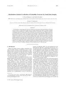
FIG. 3. Histograms of the distribution of the number of rain areas as a function of rain-area size (square root of the area, expressed in grid points, where 1 grid point ⫽ 22 km) for (a) stage IV and (b) WRF. All forecasts are initialized at 0000 UTC during the period July–August 2001.

points and 2.5 mm, respectively). While the results would vary as a function of these parameters, these particular choices lead to objects that are representative of the precipitation objects that are likely to be resolved by a 22-km model. Additional parameter combinations will be investigated in future studies.

a. Size distribution The statistical distribution of rain-area size is shown in Fig. 3 for both stage-IV and WRF forecasts. In all, we found approximately 3600 observed rain areas and 3200 forecast areas. As noted previously, areas of less than

JULY 2006

DAVIS ET AL.

1779

FIG. 4. Spatial density of rain areas computed from Wij ⫽ 兺m exp(d2m /s2), where s ⫽ 7.5 grid points, and d is the distance separating each grid point (of the WRF 22-km grid) and rain-area pair dm ⫽ [(xij ⫺ xm)( yij ⫺ ym)]1/2; (a) stage-IV rain-area density at 0900 UTC; (b) stage-IV rain-area density at 2100 UTC (21-h forecasts); (c) same as in (a) but for WRF (21-h forecasts); and (d) same as in (b) but for WRF (33-h forecasts).

25 grid cells (size ⫽ 5 grid cells) were removed from further consideration. Thus the total number of rain areas shown in Fig. 3 is about 2500 forecast and 3000 observed. The observations contain a larger number of small rain areas with a more rapid decrease in the number of rain areas with increasing size compared to WRF. The peak in the observations occurs near a size of nine grid points, or areas characterized by a length scale of about 200 km. This peak may be exaggerated owing to the smoothing inherent in convolution. When examined on a finer grid (see Part II) no peak is evident near the same dimensional size. The WRF model has an excess of larger rain areas that is especially pronounced for size ⬎30 grid points (⬃660 km). It is probable that WRF, with its effective resolution of perhaps 6–8 times the grid increment (Skamarock 2004), or about 150–200 km, fails to resolve gaps between multiple rain areas that are nearby. Also contributing to the WRF error in size distribution is a positive bias in the lower percentiles of rainfall (section 4). Because of the thresholding used to define

rain areas, this bias could also result in larger predicted areas in WRF.

b. Spatial distribution To examine the spatial distribution of rain areas, we computed a summation of the weighting function exp(⫺d2m /s2) at each grid point, where dm is the distance between a given grid point and the centroid of the mth rain area, expressed as a number of grid points. The decay scale factor s ⫽ 7.5 corresponds to about 150 km and yields a smooth distribution whose basic features are well resolved by both forecasts and observations. Essentially, the result can be interpreted as the number of rain areas located within roughly 150 km from each grid point. We stratify the data according to time of day, so for a given time of day, the maximum sum is 62 for the months of July and August. Figure 4 reveals the distributions of forecast and observed rain areas. In summary, during the nighttime (0900 UTC), WRF predicted too few rain areas over southern Arizona and the High Plains and too many

1780

MONTHLY WEATHER REVIEW

VOLUME 134

FIG. 5. (a) Fraction of bounding rectangle with rainfall greater than 2.5 mm in 3 h; (b) median angle (with respect to east–west alignment) in degrees; and (c) mean aspect ratio of rain areas. All are functions of the size of the rain area (see Fig. 3).

rain areas over the Gulf Coast states. During the afternoon (2100 UTC), WRF predicted too few rain areas over the Mid-Atlantic region and the Gulf Coast and too many rain areas over the High Plains. As shown in Fig. 4, the diurnal cycle of rainfall systems is generally poorly handled over the High Plains. This result is broadly consistent with the result obtained from examination of time–space diagrams of rainfall (Davis et al. 2003). The results of the rain-area distribution combined with the space–time diagrams suggest that the WRF produces too few propagating organized rainfall systems (e.g., mesoscale convective systems) initiating over the western High Plains during the afternoon and propagating eastward overnight. When WRF produces nocturnal systems, they tend to be too large (see also Part II). In addition, the morning minimum of convection initiation over elevated terrain is connected to an observed rain-area minimum over the High Plains in the early afternoon that is not represented in WRF. The rain-area diagnostic also reveals errors in convection associated with the thermally forced land–seabreeze system near the Gulf Coast. WRF shows significantly smaller amplitude in its diurnal variation of rain areas. Part of the low bias in the number of afternoon rain areas near the Gulf Coast results from WRF combining a number of smaller rain areas into a small number of larger areas. This is also consistent with WRF’s positive bias for lower intensity rainfall values (section 4). That is, lighter rainfall spread too widely will result

in fewer, larger rain areas unless a high rainfall threshold is chosen for filtering.

c. Other parameters Shown in Fig. 5 are three examples of additional parameters that can be investigated with our approach. The fraction of area covered (Fig. 5a) is simply the ratio of the number of grid points that survive the convolution and thresholding process to the area of the minimum, bounding rectangle. This ratio provides a measure of the regularity of the object shapes. This number seems relatively invariant for smaller objects, about 0.65, but decreases in size for larger objects. Overall, the pattern of this parameter for the WRF forecasts appears to be well matched to the pattern for the stageIV objects. Note that the ratio of a circle or ellipse to the smallest bounding rectangle is ␲/4 (⬃0.79), hence, the fractional area is smaller than would result from elliptical rain areas and the model deviates from this effective upper bound by the same amount as is observed. The median angle indicates how rain areas are oriented relative to the east–west direction (an angle of zero). Given that the maximum possible offset is 90°, the error of 20° at small scales (Fig. 5b) is particularly notable. Because the median angle of observed systems is nearly zero, the WRF bias implies that the model orients its areas southwest–northeast too frequently. This bias may indicate an overproduction of frontally forced rain areas, since fronts are typically aligned

JULY 2006

1781

DAVIS ET AL.

southwest–northeast as well. The orientation angle is sensitive to subtle variations in objects that have aspect ratios near unity. However, the fact that WRF has aspect ratios farther from unity than observed for small rain areas suggests that the bias in orientation angle for those same areas is robust. Finally, the median aspect ratio shows a positive bias (Fig. 5c), though rather small, for WRF at small scales, roughly coincident with the range of sizes for which there is a positive bias in the orientation angle. This result indicates that WRF tends to produce rain areas that are more elongated than the observed areas, which could again indicate an excess of frontally forced precipitation.

4. Statistics of matched objects Using the matching condition described in section 3, namely, that the separation between centroids of two objects be less than the sum of their sizes, we computed statistics for matched areas during July–August 2001 from the WRF 22-km grid and stage-IV analyses. In many cases, matched objects each contain multiple rain areas. We considered mean and standard deviation of errors in the following parameters: centroid position (x–y), area, and intensity. The area is computed from the number of grid points within an object that have nonzero rainfall. Intensity biases are assessed for both the 25th and 90th percentile rain rates. The biases for area and each intensity percentile are normalized by the respective average values of each quantity as described below. We also consider the object-based CSI, defined as the number of pairs of matched objects divided by the sum of the number of matches, misses (observed objects that are not forecast) and false alarms (forecast objects that do not occur). Object-based CSI (hereafter simply CSI) will be considered as a function of both forecast lead time and of the square root of the area of the larger of the two matched objects. Figure 6 shows two curves of CSI for two values of threshold separation distance used to define a match. The “standard” threshold (also used to compute results 1/2 shown in Fig. 8) is Dc ⫽ A1/2 f ⫹ Ao as defined in section 2. We also consider D* c ⫽ 1/2Dc. One expects significant error growth during a 48-h forecast of rainfall. The CSI using the less restrictive threshold Dc is rather noisy and exhibits no obvious overall trend. The “sawtooth” pattern is a result of a diurnal signal in CSI, with slightly higher values near 0000 UTC than at other times (not shown). The apparent 12-h periodicity results from inclusion of both 0000 and 1200 UTC forecast cycles in the statistics.

FIG. 6. The CSIs for matched areas as a function of forecast lead time (h). Two matching conditions are considered: centroid separation D less than the sum of the forecast and observed object sizes (solid) and D ⬍ the average of the two object sizes (dashed). Size is the square root of the object area.

The CSI for the more restrictive threshold for matching D* c exhibits a slight decrease with time. A similarly slow growth of errors for convection forecasts has been noted by Fowle and Roebber (2003) and Done et al. (2004). The lack of error growth early in the forecast is likely a result of unsuccessful initialization of ongoing precipitation systems, in turn, due to the simple interpolation from the Eta forecast without additional assimilation; hence, errors start out large. Relatively slow error growth at later times may indicate that rain areas are linked with larger-scale systems, as found in Fowle and Roebber (2003) and Done et al. (2004). There is a statistically significant positive bias of forecast object size at all forecast lead times (not shown). Because the area itself varies diurnally, the area bias has been normalized by the average of all matching observed areas for a given time of day, that is,

兺 关A ⫺ A ⫽ 兺A 共h兲 f,i

h兲 B 共area

共h兲 o,i 兴

i

共h兲 o,i

.

i

Here, the subscripts f and o refer to forecast and observations, respectively, superscript h refers to the hour of the day, and the sum is over all matching pairs at a given hour. Hence, B is simply the usual definition of bias with unity subtracted. For B ⫽ 0, there is no bias. As indicated in Fig. 7a, the area bias has a strong diurnal dependence. The WRF tends to drastically overestimate the size of rain areas during the day, whereas at night its bias is smaller, though still statistically significant. Here significance is evaluated using the Student’s t test (Wilks 1995) for the difference of means of the forecast and observed distributions of

1782

MONTHLY WEATHER REVIEW

VOLUME 134

FIG. 8. CSI for matching as a function of object size (square root of the area).

FIG. 7. (a) Area bias (WRF–stage IV) as a function of time of day (UTC), normalized by the average of all forecast and observed areas at that time; (b) bias in 25th and 90th rainfall rate percentiles, also as a function of time of day. In (b) rainfall biases have been normalized by mean 25th and 90th observed rainfall percentiles, respectively.

sizes, with the null hypothesis that the means are indistinguishable. A 0.01 probability of a type-I error (i.e., probability of incorrectly rejecting the null hypothesis) is allowed. Both the observations and WRF have a systematic diurnal variation of rain-area size, but WRF exaggerates the amplitude of this variation in addition to having a systematic positive size bias. The diurnal cycle of area bias correlates with the variation of intensity biases. In analogy with the treatment of area errors, we compute the statistic

兺 关R ⫺ R ⫽ 兺R 共N兲 f,i

N兲 B 共intensity

共N兲 o,i 兴

i

共N兲 o,i

i

for the error in the Nth percentile rainfall R(N). As shown in Fig. 7b, the 25th percentile in WRF is overestimated while the 90th percentile is underestimated. Again, the biases are statistically significant at all times. Put another way, the predicted distributions of rainfall are too narrow compared with observations. The bias in the width of the distribution is greatest during the late afternoon. It turns out that the bias in the median rainfall is also systematically positive (not shown), and generally coincides with the bias in size (Fig. 7a), potentially accounting for much of the overall positive rain-

fall bias in WRF during this period noted by Davis et al. (2003). We speculate that the excessively narrow predicted distribution of rainfall is a result of parameterized convection. The bias is greatest during the late afternoon when the thermodynamic destabilization of the atmosphere is greatest (2100–0000 UTC). We have observed that the variance of rainfall within regions of parameterized convection is typically smaller than in regions where explicitly simulated rainfall is significant. This may occur because single-column schemes (i.e., most convective schemes) have relatively few degrees of freedom. The Betts–Miller–Janjic scheme is mainly an adjustment scheme, and is not designed to represent the observed statistical variability of rainfall. In the present case, the convection scheme has an additional bias of being overly active. Rain areas predicted late at night have smaller intensity and size errors, but there is no evidence that the model has an increased ability to match observed, nocturnal rain areas. In fact, as shown in Fig. 4, there are first-order errors in the predicted locations of nocturnal rain areas. Last, we show the dependence of CSI values for matched objects on the size of the larger area (forecast or observed; Fig. 8). One matching threshold is the standard defined for Fig. 6 (D ⬍ Dc), but we also consider distance thresholds that are constant (9 and 18 grid lengths, or 198 and 396 km). Matching has a strong dependence on object area, as might be expected. Areas with a length scale of roughly 15 grid lengths or greater (330 km) have a high probability of being matched, whereas those whose length scale is on the order of 6–10 grid lengths (132–220 km) have little chance of being matched. The curves for constant distance thresholds also suggest a strong variation of prediction capability as a function of object size. While the number of large objects is modest (e.g., Fig. 3), the

JULY 2006

DAVIS ET AL.

curves representing distance-independent matching conditions in Fig. 8 suggest a plateau of CSI values for sizes greater than about 17 grid lengths (374 km). While there may be many factors contributing to the curves shown in Fig. 8, one of the leading possibilities is that larger rain areas are produced in conjunction with well-defined synoptic and mesoscale features that can be analyzed and predicted with considerable skill. Smaller rain areas may arise from more localized features (outflow boundaries, the dry line, etc.) that are less predictable and whose attendant rain areas suffer from even lower predictability.

5. Summary and conclusions We have described an object-based verification methodology applied to forecasts of rainfall during the warm season over the continental United States (CONUS). The method targeted mesoscale areas of precipitation by performing a convolution and thresholding operation that (i) yielded contiguous precipitation areas and (ii) filtered out isolated cells or areas of very light rain. The convolution and thresholding parameters can be adjusted to verify precipitation forecasts on different spatial or temporal scales. Once rain areas were identified, their attributes, including centroid location, size, orientation, curvature, and intensity distribution were computed. We performed a statistical comparison of attributes of rain areas identified in WRF forecasts run on a 22-km grid covering the CONUS during July–August, 2001, and rain areas identified in gridded stage-IV precipitation data from NCEP for the same period (coarsened to the model grid). Notable systematic model errors were: (i) WRF produced too many large (length ⬎400 km) areas of precipitation and insufficient small (length ⬍200 km) areas; (ii) WRF rain areas were too elongated; and (iii) WRF exhibited major regional errors in the temporal frequency of rain areas as a function of time of day, missing a nocturnal maximum over the plains states (consistent with results shown by Davis et al. 2003) and underrepresenting the diurnal variation near the Gulf of Mexico. We used a simple method for matching forecast and observed rain-area pairs based mainly on the separation of their centroids relative to the sum of their sizes. The most prominent errors for matched objects were an overprediction of area size in WRF that varied diurnally, with the largest overprediction being during the time of maximum daytime heating when the atmosphere was most unstable. This coincided with a narrowing of the rainfall intensity distribution relative to

1783

that observed, which we interpreted as variance damping due to parameterized convection. In addition, matching skill increased sharply with object size. This trend was interpreted as a consequence of dominant mesoscale or synoptic-scale influences on organization of larger areas, and local processes influencing smaller areas. The object-based verification approach described herein shows promise as a way to alleviate some of the problems and issues associated with current QPF and convective forecast verification techniques. Additional important issues remain, however, including development of methods to separate and evaluate the various scales of the forecasts and observations. New applications of wavelet techniques to this problem are under development (e.g., Casati et al. 2004) and may help untangle this issue. In addition, more sophisticated tools for matching forecast and observed objects are needed and will be an important focus of the next phase of the object-based verification work. Eventually, the object-based methodology may be tied together with alternative verification approaches such as the method developed by Ebert and McBride (2000) to decompose forecast errors into meaningful diagnostic components; the classification approach being developed by Baldwin and Lakshmivarahan (2003); and the “perfect hindcast” approach described by Brooks et al. (1998). In Part II, we extend our rain-area methodology to examine fully explicit forecasts of convective systems. We also consider temporal matching of rain areas, both to identify rain systems (temporally coherent collections of rain areas), and to quantify forecast timing errors. By adjusting the convolution and thresholding parameters, and considering the intensity distribution within areas, we can distinguish strongly convective rain patches from lighter rain areas. Development and application of this verification approach will lead to the availability of much more informative results from verification studies of precipitation and convective forecasts (and the approach may be useful for a variety of other forecast elements as well). As the technique matures it will be able to meet the decision-making needs of a wide variety of users while also providing diagnostic information to forecast developers. Acknowledgments. This work was supported through funding from the U.S. Weather Research Program and the Air Force Weather Agency. The authors acknowledge contributions from Beth Ebert from BMRC, and Rebecca Morss, Daran Rife, Kevin Manning, Agnes Takacs, Mike Chapman, Eric Gilleland, John Halley Gotway, and Dave Albo of NCAR.

1784

MONTHLY WEATHER REVIEW REFERENCES

Baldwin, M. E., and S. Lakshmivarahan, 2003: Development of an events-oriented verification system using data mining and image processing algorithms. Preprints, Third Conf. on Artificial Intelligence Applications to Environmental Science, Long Beach, CA, Amer. Meteor. Soc., CD-ROM, 4.6. Black, T. L., 1994: The new NMC mesoscale Eta model: Description and forecast examples. Wea. Forecasting, 9, 265–278. Brooks, H. E., M. Kay, and J. A. Hart, 1998: Objective limits on forecasting skill of rare events. Preprints, 19th Conf. on Severe Local Storms, Minneapolis, MN, Amer. Meteor. Soc., 552–555. Casati, B., G. Ross, and D. B. Stephenson, 2004: A new intensityscale approach for the verification of spatial precipitation forecasts. Meteor. Appl., 11, 141–154. Case, J. L., J. Manobianco, J. E. Lane, C. D. Immer, and F. J. Merceret, 2004: An objective technique for verifying sea breezes in high-resolution numerical weather prediction models. Wea. Forecasting, 19, 690–705. Davis, C. A., K. W. Manning, R. E. Carbone, J. D. Tuttle, and S. B. Trier, 2003: Coherence of warm season continental rainfall in numerical weather prediction models. Mon. Wea. Rev., 131, 2667–2679. ——, B. Brown, and R. Bullock, 2006: Object-based verification of precipitation forecasts. Part II: Application to convective rain systems. Mon. Wea. Rev., 134, 1785–1795. Done, J., C. Davis, and M. Weisman, 2004: The next generation of NWP: Explicit forecasts of convection using weather research and forecast (WRF) model. Atmos. Sci. Lett., 5, 110–117. Doswell, C. A., R. Davies-Jones, and D. L. Keller, 1990: On summary measures of skill in rare event forecasting based on contingency tables. Wea. Forecasting, 5, 576–585. Ebert, E., and J. L. McBride, 2000: Verification of precipitation in weather systems: Determination of systematic errors. J. Hydrol., 239, 179–202. Fowle, M. A., and P. J. Roebber, 2003: Short-range (0–48 h) numerical prediction of convective occurrence, mode, and location. Wea. Forecasting, 18, 782–794. Fulton, R. A., J. P. Breidenbach, D.-J. Seo, D. A. Miller, and T.

VOLUME 134

O’Bannon, 1998: The WSR-88D rainfall algorithm. Wea. Forecasting, 13, 377–395. Hong, S.-Y., and H.-L. Pan, 1996: Nocturnal boundary layer vertical diffusion in a medium-range forecast model. Mon. Wea. Rev., 124, 2322–2339. Mahoney, J. L., B. G. Brown, J. E. Hart, and C. Fischer, 2002: Using verification techniques to evaluate differences among convective forecasts. Preprints, 16th Conf. on Probability and Statistics in the Atmospheric Sciences, Orlando, FL, Amer. Meteor. Soc., 12–19. Michalakes, J., S. Chen, J. Dudhia, L. Hart, J. Klemp, J. Middlecoff, and W. Skamarock, 2001: Development of a next generation regional weather research and forecast model. Developments in Teracomputing: Proceedings of the Ninth ECMWF Workshop on the Use of High Performance Computing in Meteorology, W. Zwieflhofer and N. Kreitz, Eds., World Scientific, 269–276. Murphy, A. H., 1991: Forecast verification: Its complexity and dimensionality. Mon. Wea. Rev., 119, 1590–1601. ——, 1993: What is a good forecast? An essay on the nature of goodness in weather forecasting. Wea. Forecasting, 8, 281– 293. Nachamkin, J. E., 2004: Mesoscale verification using meteorological composites. Mon. Wea. Rev., 132, 941–955. ——, S. Chen, and J. Schmidt, 2005: Evaluation of heavy precipitation forecasts using composite-based methods: A distributions-oriented approach. Mon. Wea. Rev., 133, 2163–2177. Rife, D. L., and C. A. Davis, 2005: Verification of temporal variations in mesoscale numerical wind forecasts. Mon. Wea. Rev., 133, 3368–3381. Ritter, G. X., and J. N. Wilson, 2001: Computer Vision Algorithms in Image Algebra. CRC Press, 417 pp. Skamarock, W. C., 2004: Evaluating mesoscale NWP models using kinetic energy spectra. Mon. Wea. Rev., 132, 3019–3032. Smith, B. B., and S. L. Mullen, 1993: An evaluation of sea level cyclone forecasts produced by NMC’s nested-grid model and global spectral model. Wea. Forecasting, 8, 37–56. Wilks, D. S., 1995: Statistical Methods in the Atmospheric Sciences. Academic Press, 467 pp.