JULY 2006
1785
DAVIS ET AL.
Object-Based Verification of Precipitation Forecasts. Part II: Application to Convective Rain Systems CHRISTOPHER DAVIS, BARBARA BROWN,
AND
RANDY BULLOCK
National Center for Atmospheric Research,* Boulder, Colorado (Manuscript received 20 December 2004, in final form 7 October 2005) ABSTRACT The authors develop and apply an algorithm to define coherent areas of precipitation, emphasizing mesoscale convection, and compare properties of these areas with observations obtained from NCEP stage-IV precipitation analyses (gauge and radar combined). In Part II, fully explicit 12–36-h forecasts of rainfall from the Weather Research and Forecasting model (WRF) are evaluated. These forecasts are integrated on a 4-km mesh without a cumulus parameterization. Rain areas are defined similarly to Part I, but emphasize more intense, smaller areas. Furthermore, a time-matching algorithm is devised to group spatially and temporally coherent areas into rain systems that approximate mesoscale convective systems. In general, the WRF model produces too many rain areas with length scales of 80 km or greater. Rain systems typically last too long, and are forecast to occur 1–2 h later than observed. The intensity distribution among rain systems in the 4-km forecasts is generally too broad, especially in the late afternoon, in sharp contrast to the intensity distribution obtained on a coarser grid with parameterized convection in Part I. The model exhibits the largest positive size and intensity bias associated with systems over the Midwest and Mississippi Valley regions, but little size bias over the High Plains, Ohio Valley, and the southeast United States. For rain systems lasting 6 h or more, the critical success index for matching forecast and observed rain systems agrees closely with that obtained in a related study using manually determined rain systems.
1. Introduction Brooks and Doswell (1996) have remarked that a lack of systematic verification of forecasts is “an implicit admission that the quality of the forecasts is of low priority.” Measures-based statistics arguably fail to provide useful information about the quality of forecasts of highly intermittent, spatially localized phenomena, especially as the richness of the simulated phenomenological spectrum increases. Most so-called high-resolution, regularly produced forecasts today (including most real-time and operational forecasts) are verified using measures-based approaches. By the above reasoning, one might conclude that there is little priority placed on the quality of such forecasts. Because
* The National Center for Atmospheric Research is sponsored by the National Science Foundation.
Corresponding author address: Christopher A. Davis, National Center for Atmospheric Research, P.O. Box 3000, Boulder, CO 80307. E-mail:
[email protected]
© 2006 American Meteorological Society
MWR3146
we do not believe that this is the case, we echo the sentiment of Murphy (1993) regarding the importance of verification approaches that probe the joint distribution of forecasts and observations, thereby yielding a more complete picture of the nature of forecast errors. The large dimension of forecast models, often 107– 8 10 variables, makes full evaluation of the joint distribution of forecasts and observations practically impossible. First, observations are totally inadequate for this task, but even if they were adequate, the magnitude of the dimension would make it exceedingly difficult to distill results to the point where interpretation was possible. To reduce this dimension, a number of simplifications are required, each involving assumptions that contain some degree of arbitrariness whose adverse affect can only be estimated in hindsight. One such approach, the decomposition of forecasts into discrete, phenomenologically based objects, is considered herein. In this paper, we focus on warm season rainfall forecasts from the new Weather Research and Forecasting model (WRF; Michalakes et al. 2001). Rainfall is useful as a quantity to verify because (i) it is a highly discrimi-
1786
MONTHLY WEATHER REVIEW
nating aspect of numerical forecasts; (ii) rainfall has obvious practical significance for a variety of forecast users, including meteorologists, decision makers, and the general public; and (iii) at least over the continental United States, rainfall patterns are observed with exceptional temporal and spatial resolution owing to the national network of radars and rain gauges. The verification challenge is that rainfall is localized and episodic (though with some remarkable diurnal repeatability), rendering traditional analysis and verification approaches problematic. However, these qualities make rainfall an ideal candidate for object-based approaches that reduce drastically the dimension of the verification problem by identifying coherent or contiguous entities with characteristic attributes. The method for identification and verification of contiguous rain areas is related to the method developed by Ebert and McBride (2000), and is broadly similar to strategies considered by Baldwin and Lakshmivarahan (2003). The basic approach is described by Davis et al. (2006, hereafter Part I), and is extended here to include matching of rain areas in time in order to define rain systems, analogous to mesoscale convective systems (MCSs). Herein we consider forecasts performed with a grid spacing of 4 km, versus the 22-km grid spacing of forecasts evaluated in Part I. Thus, the convection in the present forecasts is treated explicitly and motions are resolved on scales 5–6 times smaller than in Part I. A brief overview of the verification method appears in section 3. We then break the results into three distinct verification pieces: separate forecast and observed distributions of rain areas, distributions of forecast and observed rain systems, and characteristics of matched rain systems (sections 4, 5, and 6, respectively). The purpose of considering distributions from the populations of forecast and observed areas separately is to compare the results with those in Part I. The definition of rain systems and the statistics of matched systems will also be compared with results obtained by Done et al. (2004, hereafter DDW), who examined a subset of the data used herein by manually identifying and comparing MCSs in the forecasts and observations. We will show that the attributes of rain areas have some distinct functional dependencies on size (or duration, in the case of rain systems). Further, we will obtain some conclusions regarding the skill of the WRF model in predicting rain systems that are qualitatively similar to those found by DDW. This similarity occurs despite a notable discrepancy in the members of the forecast and observed rain systems (MCSs) identified by the automated and manual approaches. We close with a further comparison of automated and manual verification approaches.
VOLUME 134
2. Data Forecasts were obtained from a complete set of realtime forecasts by the Eulerian mass-coordinate version of the WRF model (release 1.3) between 3 May and 15 July 2003.1 Each forecast was initialized at 0000 UTC by interpolation of the corresponding cycle of the Eta model (Black 1994) from the National Centers for Environmental Prediction (NCEP). The forecasts were integrated for 36 h using the Eta for lateral boundary conditions. The forecasts were integrated on a 4-km grid on a domain containing 500 ⫻ 500 points in the horizontal plane with 34 vertical levels (see DDW for more details). The precipitation field was output as hourly accumulations. As in DDW, herein we only consider forecasts from 12 to 36 h to avoid redundancy (i.e., overlap between successive forecasts). Note that DDW used maximum reflectivity in a column to identify MCSs. The observed precipitation was derived from the stage-IV precipitation analyses from NCEP (Baldwin and Mitchell 1997), obtained on a 4-km grid at hourly increments for the entire period. Because the 4-km stage-IV grid was not identical to the WRF grid, some interpolation was required to map the observations onto the WRF grid. This was done as in Part I so that the volume integral of the observed precipitation was preserved.
3. Method a. Rain areas The method we adopt is described in more detail in Part I, but an overview is presented here. There are three distinct steps in the method, results of which are displayed in corresponding sections 4, 5, and 6, respectively. The first task is to filter the rainfall field and define rain areas. The filtering is done in a two-step process. First, the entire field is convolved with a disk whose radius is closely tied to the minimum scale well resolved by the model or observations. The particular convolution (smoothing in our application) chosen replaces the value of a field at a given point by its average over all grid points within a distance R. Herein, the convolving disk has a radius of four grid lengths (16 km), the same number of grid lengths assumed for R in Part I (wherein four grid lengths equaled 88 km). The convolution disk radius can, in principle, be greater, but we find empirically that this choice yields rain areas similar to what a human would identify. 1 The study by DDW considered the same forecast and observation sources, but only from 13 May to 9 July 2003.
JULY 2006
DAVIS ET AL.
1787
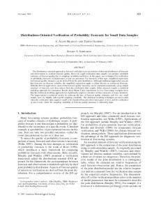
FIG. 2. Same as in Fig. 1, but after convolution and thresholding (5 mm h⫺1). FIG. 1. Grayscale image of 1-h rainfall accumulation (mm) valid 0400 UTC 11 Jun 2003 (28-h forecast).
After convolving the raw field, we retain only those points that exceed a threshold of 5 mm h⫺1. This effectively removes areas of light precipitation. An example of the raw field, and the resulting field after the convolution and thresholding processes have been applied, are shown in Figs. 1 and 2, respectively. The combination of convolution and thresholding yields fewer, larger contiguous areas of precipitation than a simple thresholding would do. It is still possible that small precipitation areas will result, but in the remainder of this paper, we will only consider contiguous areas of 25 grid cells (400 km2) or greater. Although the original rainfall was smoothed and thresholded to define rain areas, we retain the original rainfall values at those points that remain nonzero after filtering. In this way, we can examine statistics of the rainfall intensity as another object attribute. We take this approach rather than considering pointwise prediction of rainfall because, to first order, prediction of rainfall intensity at a point is a stochastic problem during the warm season. As described in Part I, we define several attributes of rain areas. Each area is identified by a time, centroid location, size, major axis, minor axis, orientation angle between the approximate east–west direction and the major axis, and the rainfall intensity distribution. Derived parameters are also computed. The fraction of area covered is defined as the ratio of area with rainfall
greater than zero (after convolution and thresholding) to the product of major and minor axis lengths. It is indicative of the complexity of the rain-area shape, being smaller for areas that have “holes” within them or highly irregular outlines. Aspect ratio, the ratio of minor to major axis lengths, can indicate whether a rain area is organized by a quasi-linear feature such as a front or coastline. For more intense systems dominated by convection, the aspect ratio can indicate whether a well-defined convective line is present.
b. Rain systems A sequence of rain areas at consecutive times can be discrete realizations of a single, coherent, translating, rain system. For example, MCSs are recognized as much by their characteristic time evolution and temporal coherence as by their instantaneous appearance. It is useful to develop ways to identify rain systems that are analogous to time contiguous systems identified by meteorologists so that the model evaluation is phenomenologically based and also so that meaningful statistics about timing errors can be derived. Herein we define rain systems by matching rain areas separated temporally by 1 h if their centroids are separated by less than a threshold distance. Upon completing one pass through the dataset, we obtain all rain systems lasting at least 2 h (Fig. 3). We denote the duration of these by the index k (⫽2). The attributes (e.g., size, area, intensity, etc.) of matched areas are
1788
MONTHLY WEATHER REVIEW
FIG. 3. Schematic, in one spatial dimension, of time matching of rain areas to produce rain systems. Symbols indicate centroids of original rain areas (open circles), systems lasting 2 h (stars), systems lasting 3 h (squares), and the single system of 4-h duration (filled circle) that results from merging all four of the original rain areas.
averaged to define the attributes of the corresponding rain system. After one pass, all remaining unmatched rain areas are assigned a duration of 1 h (k ⫽ 1). The set of 2-h rain systems is treated as a new set of rain areas, and in the next pass through the data, these are matched based on spatial proximity and a 1-h time displacement, yielding all rain systems lasting at least 3 h (k ⫽ 3) and a set of unmatched systems whose duration is 2 h (k ⫽ 2). The process is repeated until we have grouped all the original rain areas into rain systems with duration ranging from 1 h to, in this case, about 16 h, corresponding to the longest-lived rain system in the dataset. The sequential averaging produces attributes of the final rain system that are linear combinations of the attributes of the original areas. For k ⫽ 2, the properties of two areas are averaged to obtain the properties of the rain system lasting 2 h. The weighting may be expressed as (1⁄2, 1⁄2). For k ⫽ 3, three rain areas are averaged and the weighting is (1⁄4, 1⁄2, 1⁄4). For k ⫽ 4 the weighting is (1⁄8, 3⁄8, 3⁄8, 1⁄8). Thus, the attributes near the middle of the system life cycle receive more weight than attributes near the beginning or ending. Therefore, the attributes will typically represent the mature stage of a system more than the initiation or dissipation stages. The mean translation speed, however, is simply the difference in endpoint positions divided by the duration. The threshold centroid displacement used for matching two rain areas separated by 1 h in time can be interpreted as a maximum allowed translation speed.
VOLUME 134
We set this threshold to 40 m s⫺1, or 144 km h⫺1, and it is applied to the centroids of each rain area. This upper bound is consistent with the most rapid ground-relative movement of MCSs observed (e.g., Carbone et al. 2002). Westward movement nullifies a match. While it may be desirable to allow westward movement in some cases, in practice it is difficult to distinguish westward movement from the formation of a separate upstream system based solely on hourly rainfall. To distinguish areas with appreciable deep convection from weaker rain areas, we require that all rain areas have a 75th percentile rain rate greater than the median value for the entire sample (evaluated separately for forecast and observed rain areas). The speed and intensity criteria must be met at all times during the existence of a rain system. For simplicity, we only consider the nearest rain areas (or rain systems, if k ⬎ 1) for matching.
c. Matching rain systems In general, we define a centroid for an object (a rain system) in (x, y, t) space as (xo, yo, to) or (xf, yf, tf) depending on whether it is observed or forecast, respectively. All attributes are defined at these centroid locations. The forecast “position” error is just (xf ⫺ xo, yf ⫺ yo, tf ⫺ to). Thus, time t and space x, y errors are formally separated. If a forecast object has its centroid in the correct geographical location, but is displaced in time, the error is one of timing. If the forecast system correctly predicts its temporal centroid, but predicts the spatial centroid in the wrong geographical location, the error is spatial. If everything propagates at the same speed c, such that x ⫺ ct ⫽ constant, for example, then either the “x” or “t” dimension can be considered redundant, and the dimensionality reduces to two. Verification in this reduced-dimensional space was considered in Davis et al. (2003). In practice, however, different systems have widely varying translation velocities and all three components (x, y, t) are independent to a significant degree. To match forecast and observed rain systems, we adopted simple criteria that are similar to those employed by DDW. Rain systems were matched if • the centroids of the forecast and observed systems
were within a distance equal to 4 times the average of the short-axis lengths of the two areas: [(xf ⫺ xo)2 ⫹ (yf ⫺ yo)2] ⬍ 4L, where L ⫽ 1/2(Lf ⫹ Lo) and L is the short-axis length; • the average times of the two systems differed by not more than 3 h: | tf ⫺ to | ⬍ 3 h; • the duration k of the observed system was between 0.5 and 2 times the forecast system duration: 0.5 ⱕ ko/kf ⱕ 2.
JULY 2006
DAVIS ET AL.
1789
FIG. 4. (a) Natural log of the number of rain areas vs size, plus symbols for WRF and circles for observations; (b) same as in (a) but for fractional area; (c) same as in (a) but for aspect ratio; and (d) angle of major axis with respect to the east–west grid direction.
The criterion for time difference was the same used by DDW, and ensured that matched systems occurred during the same phase of the diurnal cycle. The distance condition was similar to that applied by DDW. However, the short-axis length varied significantly with mean system duration, ranging from about 60 km for short-lived systems, to over 100 km for long-lived, larger systems. The average value for systems lasting 3 h or more was roughly 80 km, and 4 times this value (320 km) was close to the distance threshold used by DDW (333 km). The restriction on duration was somewhat arbitrary, but was designed to discount systems of such different duration that they may be governed by different dynamics. This condition differed from that used by DDW wherein all MCSs, both observed and forecast, were required to last at least 6 h. Such a restriction will be shown to limit the computed forecast skill. The median intensity of rain systems was not used as a matching condition because intensity was used to define the original rain areas.
4. Statistics of rain areas As in Part I we computed statistics of rain areas, first without consideration of matching or time dependence (statistics of rain systems will appear in section 5). Herein we group rain areas by size, defined as the
square root of the number of grid cells with rainfall greater than 5 mm h⫺1. Other attributes could be chosen as the independent variable, but the horizontal length scale is chosen because it often discriminates different dynamics and predictability. The number of rain areas depends strongly on size (Fig. 4a). Both WRF and stage-IV rain areas exhibit a similar quasiexponential dependence of the number of areas as a function of size. Both distributions peak near a size of seven grid cells or 28 km. This peak is probably artificial, being the result of convolution of the original data. The WRF model produces a greater number of areas with a length scale of 80–120 km than the observations. In Part I, an underprediction of rain areas between roughly 150 and 250 km was noted, with an overprediction of areas exceeding a size of about 350 km. Thus, both finer and coarser applications of WRF produced rain-area bias near the same size when measured by the number of grid points, but not in terms of physical dimension. In Fig. 4, we show the dependence of fractional area (Fig. 4b), aspect ratio (Fig. 4c), and angle of major axis orientation (Fig. 4d) on size. We place a minimum restriction on the number of objects that must occur within a given bin (40). For larger rain areas where fewer than 40 reside within a size bin, we group successive bins together until at least 40 areas are accumu-
1790
MONTHLY WEATHER REVIEW
lated. The average size of these accumulated areas determines the abscissa location. This grouping eliminates noisy behavior due to small sample size. Regarding fractional areas, we note that values near unity occur for small rain areas. A reduction of fractional area with increasing size is apparent. A qualitatively similar reduction was noted in Part I, but for larger areas than considered here, and the decay was less rapid in both forecasts and observations. For objects of nearly all sizes, WRF exhibits a positive bias in fractional area that is statistically significant with ␣ ⫽ 0.01 based on a Student’s t test (Wilks 1995; i.e., there is a 0.01 probability of incorrectly rejecting the null hypothesis that the means are indistinguishable).2 The cause of this bias may be a combination of aliasing convection onto somewhat larger scales than observed because of resolution limitations, and also the positive bias of rainfall in the model (see DDW). The aspect ratio (Fig. 4c) also has a monotonic decay with increasing size, but the decay is rapid for areas smaller than about 50 km. For larger areas, the decay is slow with aspect ratio values between 0.4 and 0.5 over a wide range of scales. The dependence of aspect ratio on size is handled well by WRF. The model has little systematic bias except for a statistically significant positive bias for small rain areas. The mean angle (Fig. 4d), measuring the departure of the long axis from an east–west orientation, is positive for all sizes. Thus, although individual areas may be oriented in various ways, the mean maintains a southwest–northeast orientation, and the rotation increases with increasing size in both datasets. There is more scatter in this plot than in others, and the standard deviations within each size bin (not shown) are relatively larger. This scatter does not allow us to attribute high statistical significance to the result. The scatter itself likely results from wide variations of angles in areas that are nearly round. The overall similarity of functional relationships identified herein with those found in Part I, for larger rain areas, suggests that the dependencies (perhaps more than the values themselves) are nearly universal properties of rain areas. Furthermore, the WRF is able to reproduce the general functional relationships, though not without statistically significant biases. It is the magnitude of the biases deduced from other models that will determine whether the WRF forecasts are relatively skillful in these attributes. Such an evaluation is an objective of further research.
2 Hereafter, statistical significance will be assessed using ␣ ⫽ 0.01.
VOLUME 134
5. Statistics of rain systems Rain systems herein are characterized by their duration k, and all parameters are displayed as functions of k in Fig. 5. To avoid durations with small numbers of systems, we have performed a similar grouping as with rain areas, herein restricting the minimum group size to 10 rain systems and assigning the duration of the group to the nearest-integer-average duration of the members of that group. There tend to be similar dependences on duration for rain systems as there were on size for rain areas. Mean size and duration are clearly positively correlated (Fig. 5c). The WRF model has a statistically significant bias in both size and intensity for rain systems of nearly all durations. The bias of orientation angle, generally positive, does not attain statistical significance. To view spatial locations of rain systems, at least statistically, we computed the number of rain systems of duration 3 h or greater within each 25 ⫻ 25 grid box (100 km ⫻ 100 km) portion of the domain (Fig. 6). Overall, the WRF model captured the concentration of rain systems in the southeast United States. However, there was a clear bias toward too many forecast systems in the east and too few in the west. Furthermore, the observed minimum concentration of systems over Oklahoma and Kansas was missed in the model. The errors in the western part of the domain were most likely due to the proximity of the lateral boundary, prescribed from the Eta model initial and forecast conditions, and the intrinsic difficulty of predicting flow features responsible for convection initiation in the lee of the Rocky Mountains. In Part I the diurnal cycle of the spatial distribution of rain areas was evaluated, but there were too few rain systems to construct analogous maps for rain systems.
6. Matching forecast and observed systems Partly motivated by the spatial distribution of rain systems, we examined matching statistics for different regions: west, central, and east. These regions each occupied one-third of the domain in the x direction, and spanned the domain in the y direction. We restricted attention to forecast rain areas of 3 h or greater duration. Statistics of several parameters were examined: the critical success index (CSI), bias of x and y centroid locations, area bias, and intensity bias (25th and 75th percentiles; Table 1). The CSI, defined as the ratio of hits to the sum of hits ⫹ misses ⫹ false alarms, measured the relative frequency of matched systems. A false alarm was a forecast rain system without a matching counterpart in the observations. A miss was counted
JULY 2006
DAVIS ET AL.
1791
FIG. 5. Rain system parameters as a function of duration: (a) natural log of the number of systems, (b) averaged angle (see text for definition), (c) area, and (d) 75th percentile of rainfall intensity. Arrows indicate that the difference between WRF and the observations is statistically significant at the 99% confidence level based on a Student’s t test. Plus signs represent the WRF and circles represent the observations.
for each observed rain system of 3 h or greater duration that had no forecast counterpart. Although forecast rain systems had to last at least 3 h to be included in regional statistics, the matching rules stated above allowed observed systems to exist for as little as 2 h. Therefore, CSI values are larger than would result if only systems of 3 h or greater duration were considered for matching. Biases, however, did not appear sensitive to the sample chosen for matching. There were some biases common to all three regions. The timing of rain systems was about an hour late. We found that this timing bias extended to even shorterlived systems where it became comparable to the duration. Thus, the temporal overlap between forecast and observed systems was often small or zero for shortlived systems. The 75th percentile of the intensity distribution had a positive bias in the forecasts as well. This was a manifestation of the overprediction of convection as noted in Part I, although it was also possible that observations miss some of the higher rainfall values because of gauge spacing or gaps in radar coverage at low altitude. Other statistics showed substantial regional variation. The values of CSI were lowest over the western part of the domain, mainly the High Plains. This ap-
peared to result directly from a failure to adequately represent orographic convection over the Rockies and its immediate downstream evolution. We suspect that this error was due to the placement of the lateral boundary, but further testing would be necessary to confirm this conjecture. Although skill over the central and eastern parts of the domain was comparable, there were large systematic position errors in both regions, particularly over the east. Based on Fig. 6, we infer that this was largely due to a displacement of the maximum frequency of systems over the southeast and excessive frequency over the Tennessee and Ohio Valleys. Many of these systems moved slowly, if at all, so spatial and temporal errors were not strongly coupled. Furthermore, the central region revealed no significant position errors, despite an even larger timing error. Hence, the position and timing errors seem generally unrelated. Other notable behavior includes the fact that forecast rain systems over the central region were too large, but not significantly so over the west and east. Over the east, the rainfall intensity distribution was particularly broad relative to observations, with the tails on both the high and low ends of the distribution extending too far. An alternative perspective was gained by segregating
1792
MONTHLY WEATHER REVIEW
VOLUME 134
TABLE 1. CSI, number of matched systems, biases in time (h), x (grid lengths), y (grid lengths), area (grid cells), and rainfall intensity percentiles (I25 ⫽ 25th percentile; I75 ⫽ 75th percentile; units are mm h⫺1) for west, central, and east subregions and for the total sample of matched rain systems (forecast duration of 3 h or more). One grid length ⫽ 4 km; one grid cell ⫽ 16 km2. The boldface numbers indicate statistically significant biases at 99% confidence or greater.
FIG. 6. Distribution of rain systems with 3 h or greater duration (based on averaged centroid position) for (a) observations and (b) WRF. The grayscale indicates counts within a 100 km by 100 km box (boxes are not overlapping).
the rain systems according to the time of day at which they occur. We considered bins of 3 h, and assign systems based on their average time, only considering systems that last 3 h or more. Given the quasi-exponential decay of the number of systems versus duration, this population was dominated by systems with duration between 3 and about 5 h. Owing to limited sample sizes, we do not present the full set of diurnal errors stratified into regions, but will occasionally refer to regional, diurnal errors in some quantities.
Region
CSI
No.
Timing
dx
dy
Area
I25
I75
West Central East Total
0.38 0.51 0.51 0.48
80 175 191 446
1.2 1.2 0.8 1.0
⫺3.9 12.4 10.4 8.8
9.4 ⫺2.5 19.3 8.9
⫺9 266 55 127
0.8 0.7 ⴑ0.3 0.3
4.0 5.2 3.9 4.4
There was a large diurnal variation in the number of matching rain systems, with the greatest number near 0000 UTC (Fig. 7a). Diurnal variation in the number of systems was greatest in the west and smallest in the east. There was also a diurnal variation in skill (CSI), with lowest values (⬃0.45) around 1200 UTC and highest values (⬃0.6) around 0000 UTC. The lower skill score for late-night and early morning systems has been noted for simulations employing cumulus parameterization (e.g., Dai et al. 1999; Davis et al. 2003; Part I). In the present case there also appeared to be some difficulty for fully explicit simulations to capture precipitation systems initiating at night. Timing biases (Fig. 7b) appeared largest for nocturnal systems and smallest for systems tied to the maximum heating. Because there were almost no systems centered on noon in the west, and few in the central region, the minimum in timing bias around 1500–1800 UTC was produced because of a small early bias in the east offsetting the late bias of fewer systems elsewhere. Spatial errors (Fig. 7c) do not show any appreciable diurnal cycle when examined for all three regions together. However, errors in the east are particularly large late at night and during the morning, yet small during the afternoon. The smaller afternoon spatial biases may result from localization of convection to the sea-breeze circulation moving northward from the Gulf of Mexico, as well convection over the higher Appalachian terrain. Other regions do not show systematic diurnal trends. Note that biases in translation speed are not systematic and are not depicted here. The error in area (Fig. 7d) was normalized by the average of observed areas at a particular time, as in Part I:
兺 关A ⫺ A ⫽ 兺A 共h兲 f,i
h兲 B共area
共h兲 o,i 兴
i
共h兲 o,i
i
,
JULY 2006
1793
DAVIS ET AL.
兺 关R ⫺ R ⫽ 兺R 共N兲 f,i
N兲 B共intensity
共N兲 o,i 兴
i
共N兲 o,i
.
i
These averages ranged from 5.1 to 6.0 mm (25th percentile) and from 14.8 to 17.2 mm (75th percentile) with the largest values occurring at night for both percentiles. The largest normalized errors were clearly in the 75th percentile, and little diurnal signal was apparent. The largest positive biases in the 25th percentile of rainfall (Fig. 7e) coincided in time and space with the likesigned errors in rain-system area. The modest overprediction of light rain and positive bias in size were consistent with the tendency of forecast MCSs to persist too long in this region noted by DDW. The excessive heavy rainfall was also consistent with the overall precipitation bias reported by DDW, manifested on many occasions as convective cells and lines being too broad. This was, in turn, attributed to the limitations of explicit treatment of convection on a 4-km grid, on which deep convection cells cannot be not fully resolved.
7. Synthesis and conclusions FIG. 7. (a) Count of matching forecast-observed rain systems (solid line) and the critical success index for matching (dashed line) as a function of the time of day. Biases of WRF relative to observations for matched rain systems appear in (b)–(e): (b) timing (h); (c) position of centroid, east–west error is solid, north– south error is dashed; (d) area, normalized by the average area of forecast and observed systems at each time; and (e) 75th percentile (solid) and 25th percentile (dashed) of rainfall intensity. The rainfall percentiles in (e) have been normalized by the mean percentile value, averaged over all observed rain systems for that time of day.
where subscripts f and o refer to forecast and observed rain systems and superscript h refers to time of day. The statistic B is simply the traditional bias minus unity. The relative error peaked during the early morning and was dominated by large biases in the central region, consistent with Table 1 (where biases are not normalized and therefore convey the physical magnitude of typical errors). This error may have resulted from systems decaying more rapidly in observations than in the forecast, hence less of the observed area survived the convolution and threshold process used to define individual rain areas. In Fig. 7e, rainfall percentile errors have been normalized by the mean percentile value, averaged over all observed rain systems for a given time of day. Thus, as in Part I, the normalized error of the Nth percentile is
We have examined rain areas and temporally contiguous groups of rain areas, called rain systems, in both numerical forecasts from the WRF model and observations. The forecasts were performed on a 4-km grid without cumulus parameterization. Our results for rain areas were compared with those in Part I, wherein coarser-resolution WRF forecasts were examined. The results for rain systems, emphasizing matched forecast– observed rain-system pairs, were compared with the manually generated convection system comparison by DDW based on a subset of the same forecasts and observations. The population of rain areas decayed exponentially with increasing size, a property not reported before. The 4-km WRF forecasts produced an excessive number of rain areas with a scale of about 80 km or more (20⌬x). For the 22-km forecasts examined in Part I, the bias became pronounced around 350 km (18⌬x). The fractional area covered decreased markedly with increasing size in both datasets, but WRF had a positive bias at nearly all sizes on the 4-km grid (statistically significant with 99% confidence beyond size ⫽ 5⌬x). For the 22-km WRF, no statistically significant bias in fractional area was found. The aspect ratio and angle showed similar trends with size in both the model and observations with biases revealing only marginal statistical significance. The
1794
MONTHLY WEATHER REVIEW
overall functional dependencies on size agreed well with those found in Part I. However, for the same size, the rain areas produced by the 4-km WRF were more elongated than in the 22-km WRF. The detailed parameter dependencies are probably affected by the use of a convolving disk for smaller rain areas (i.e., areas whose size is not much larger than the disk). The 4-km WRF model produced too many rain systems, especially those lasting more than 4 h. There were statistically significant positive biases in size and intensity. We expect some relationship between size and intensity biases owing to the thresholding process used to define rain areas. However, the 75th percentile rainfall values far exceeded the rainfall threshold and the bias was more systematic with greater statistical significance than was evident in the size bias. There were notable regional biases in the location of rain systems, with too few over the High Plains and too many over the Mississippi and Ohio Valleys. The error over the High Plains was likely due to proximity to the western (usually inflow) boundary. The excess of systems over the east may result from the model’s high rainfall bias combined with thresholding used to define rain areas. However, there may be errors in physical processes (e.g., soil moisture, planetary boundary layer parameterization) that contributed to these biases. Such factors are being investigated. We separated matching results into regional categories and also examined statistics as a function of the time of day. The west region had the lowest skill, measured by the critical success index for matching. The central and east regions exhibited similar matching skill, but different mean errors in rain-system attributes. While the WRF intensity error for the 75th percentile was positive everywhere, the error for the 25th percentile (i.e., light rain) was negative in the east and positive in the central region. Only in the central region was there a significant size error. This error may result from the model failing to decay MCSs soon enough, resulting in positive biases in longevity, x location, rainfall, and average size. The excessive longevity of forecast MCSs was noted by DDW. The diurnal cycle was dominated by higher matching skill for late afternoon and evening systems, and a positive size bias for late night and morning systems. This result contrasts with those in Part I in that the size bias occurred several hours later for coarser-resolution forecasts (using a convective parameterization). Furthermore, there was no evidence that the rainfall intensity spectrum in the higher-resolution forecasts was too narrow as was the case at coarser resolution. The excessive coverage of intense rainfall, corresponding to a longer tail on the high end of the distribution, made the overall
VOLUME 134
distribution too broad in the 4-km WRF, especially during the late afternoon. To compare better with results in DDW, who found a CSI for matching considerably lower than the overall 0.48 value herein, we restricted the sample to forecast systems of at least 6-h duration. Using the present matching criteria, the observed systems therefore had to persist for at least 3 h. The overall CSI was 0.52, still much higher than that obtained in DDW. However, the skill in the east became the lowest and the overall attribute biases in the east increased. Notably, the 25th percentile intensity bias increased and there arose a positive size bias, both statistically significant. Requiring both observed and forecast systems to last 6 h or more, the overall CSI value dropped to 0.38, a value close to the 0.3 reported by DDW. The number of matching systems (80) in 74 forecasts is consistent with results of DDW, who obtained 63 matches in 58 forecasts. However, DDW also noted a southward propagation bias that we did not find. Our interpretation of this discrepancy is that DDW focused on the leading convective line, whereas rain areas encompass both leading line and stratiform precipitation regions. As systems evolve, the motion of the two MCS components may be different, with the stratiform region (potentially containing a mesoscale potential vorticity anomaly) moving with a lower midtropospheric steering flow, and the leading line propagating along or even to the right of the lower-tropospheric shear vector. In many instances, this distinction may explain the discrepancy in propagation errors between the two studies. Overall, it is clear that some of the results obtained by manual evaluation can be reproduced through an automated technique (that naturally requires some human intervention in how it is used). There is considerable overlap in the systems we define herein with those defined by DDW, for instance, but there is almost an equal amount of discrepancy. Part of the discrepancy is due to the use of instantaneous reflectivity in the manual identification versus precipitation in the automated algorithm. Nonetheless, it would be a formidable challenge to devise a technique that truly mimics human decisions regarding the definition of organized convection. However, different rain systems would likely be identified by different human analysts, even given the same general selection criteria. Given such uncertainty, the realistic goal of object-based verification is to produce the same overall conclusions about model performance, and the causes for errors, obtained by subjective evaluation. The power in the automated approach is that a variety of stratifications of the data
JULY 2006
DAVIS ET AL.
are possible, requiring far less effort than would be required of manual evaluation. An obvious future direction for the present type of object-based verification approach would be to compare forecasts from different models, both in their statistics of object attributes, and in their ability to match observed objects along with systematic errors in those forecast-observed object pairs. The other critical avenue of work is to relate statistics derived from the object-based method directly to model deficiencies, potentially using other data sources and variables. In addition, specific statistics that are meaningful for particular end users will be investigated to help develop connections between forecast quality and value.
1795
Brooks, H. E., and C. A. Doswell III, 1996: A comparison of measures-oriented and distributions-oriented approaches to forecast verification. Wea. Forecasting, 11, 288–303. Carbone, R. E., J. D. Tuttle, D. A. Ahijevych, and S. B. Trier, 2002: Inferences of predictability associated with warm season precipitation episodes. J. Atmos. Sci., 59, 2033–2056. Dai, A., F. Giorgi, and K. E. Trenberth, 1999: Observed and model simulated precipitation diurnal cycle over the contiguous United States. J. Geophys. Res., 104, 6377–6402. Davis, C. A., K. W. Manning, R. E. Carbone, J. D. Tuttle, and S. B. Trier, 2003: Coherence of warm season continental rainfall in numerical weather prediction models. Mon. Wea. Rev., 131, 2667–2679. ——, B. Brown, and R. Bullock, 2006: Object-based verification of precipitation forecasts. Part I: Methodology and application to mesoscale rain areas. Mon. Wea. Rev., 134, 1772–1784.
Acknowledgments. The authors thank Dr. Louisa Nance of NCAR for her helpful comments. This research was sponsored by the U.S. Weather Research Program.
Done, J., C. Davis, and M. Weisman, 2004: The next generation of NWP: Explicit forecasts of convection using weather research and forecast (WRF) model. Atmos. Sci. Lett., 5, 110–117.
REFERENCES
Michalakes, J., S. Chen, J. Dudhia, L. Hart, J. Klemp, J. Middlecoff, and W. Skamarock, 2001: Development of a next generation regional weather research and forecast model. Developments in Teracomputing: Proceedings of the Ninth ECMWF Workshop on the Use of High Performance Computing in Meteorology, W. Zwieflhofer and N. Kreitz, Eds., World Scientific, 269–276.
Baldwin, M. E., and K. E. Mitchell, 1997: The NCEP hourly multisensor U.S. precipitation analysis for operations and GCIP research. Preprints, 13th Conf. on Hydrology, Long Beach, CA, Amer. Meteor. Soc., 54–55. ——, and S. Lakshmivarahan, 2003: Development of an eventsoriented verification system using data mining and image processing algorithms. Preprints, Third Conf. on Artificial Intelligence Applications to Environmental Science, Long Beach, CA, Amer. Meteor. Soc., CD-ROM, 4.6. Black, T. L., 1994: The new NMC mesoscale Eta model: Description and forecast examples. Wea. Forecasting, 9, 265–278.
Ebert, E., and J. L. McBride, 2000: Verification of precipitation in weather systems: Determination of systematic errors. J. Hydrol., 239, 179–202.
Murphy, A. H., 1993: What is a good forecast? An essay on the nature of goodness in weather forecasting. Wea. Forecasting, 8, 281–293. Wilks, D. S., 1995: Statistical Methods in the Atmospheric Sciences. Academic Press, 467 pp.