Hindawi Publishing Corporation Journal of Engineering Volume 2013, Article ID 435628, 15 pages http://dx.doi.org/10.1155/2013/435628
Research Article Object Shape Recognition Using Wavelet Descriptors Adnan Abou Nabout Faculty of Electrical, Information and Media Engineering, University of Wuppertal, Rainer-Gruenter-Str. 21, 42119 Wuppertal, Germany Correspondence should be addressed to Adnan Abou Nabout;
[email protected] Received 1 October 2012; Revised 4 March 2013; Accepted 7 April 2013 Academic Editor: Yong Man Ro Copyright © 2013 Adnan Abou Nabout. This is an open access article distributed under the Creative Commons Attribution License, which permits unrestricted use, distribution, and reproduction in any medium, provided the original work is properly cited. The wavelet transform is a well-known signal analysis method in several engineering disciplines. In image processing and pattern recognition, the wavelet transform is used in many applications for image coding as well as feature extraction purposes. It can be used to describe a given object shape by wavelet descriptors (WD). Thus, it is used to recognize objects according to their contour shape by deriving a number of WD and comparing them with the WD of stored contour patterns. For our method, we use a periodical angle function derived from an extracted object contour. In order to apply the WD, the Mexican Hat can be used as the mother wavelet. In this paper, the method of object shape recognition using wavelet descriptors is described coherently and includes details relating to the method of applying the periodical angle function and the derivation of the formulas for the Haar as well as Mexican Hat wavelet descriptors. To evaluate the results of object recognition when using wavelet descriptors taking into account the dependence on the starting point, the paper describes a sufficient method for the comparison of wavelet descriptors using the minimum distance matrix.
1. Introduction Shape representation is an important step in object recognition tasks and plays a key role in many industrial applications. The recognition of 2D flat objects (e.g., plastic seals or aluminium profiles in the automobile industry) is a prime example of the need to find an appropriate shape representation which guarantees the detection of the objects despite slight object differences. Another example is the recognition of classes of weed species in agricultural applications with the objective of using the appropriate amount and type of pesticides in order to kill the pests. The problem here is that the weeds’ shapes change significantly according to their growing stages. For the above given reasons, it is necessary to find an adequate contour description, which reflects both rough and detailed information about the object shape. In recent years, many methods for shape representation and recognition have been proposed [1–10]. An advanced review of shape representation techniques can be found in [1, 2]. One can distinguish between contouroriented and region-oriented shape description techniques. The first method describes the object outlines and the second describes the object areas. In both cases, suitable contour
and region primitives are first used in order to extract the relevant objects from a given image (e.g., Freeman codes [3], polygon lines [10], and pixels or image squares [4]). Based on this data, shape description can be performed by applying a feature vector in order to represent the given objects. Using such a feature vector, the recognition task can be solved by comparing the feature vectors of different objects. In this paper, we use contour polygons and apply feature vectors using wavelet descriptors. The most popular method related to the shape description using contour data is described in [9]. The method uses shape presentation by the so-called Fourier descriptors. The classical Fourier transform allows a loss-free transmission of an image signal in the frequency domain, but unfortunately it loses the full spatial resolution. The wavelet transform offers a good solution for this problem and additionally allows the possibility of selecting the appropriate basic functions for the signal to be analyzed. This makes the wavelet transform particularly useful for many image processing problems. The mathematical foundations of the wavelet transform were developed in the early nineties, and the term “Wavelet” was used in the 1980s for functions, which generalize the shorttime Fourier transform [11]. The multiresolution analysis
2
Journal of Engineering
(MRA) using the Orthonormal Basis Functions was introduced in 1989 [12, 13]. A comparison between the short-time or windowed Fourier transform and the wavelet transform is discussed in [14]. The wavelet transformation was used in 1996 in order to describe a contour shapes [15] method based on the theory of periodized wavelets and using the MRA in order to apply wavelet descriptors. In [16–18] similar approaches are presented, which use different coordinates to describe a given object shape. One of the unattractive properties of the wavelet transform is the dependency of the WD on the selected starting point. This problem was reported in [19] and several solutions based on fixing the starting point were discussed. Hu et al report a solution using Zernike moments [19]. In this paper, we present the derivation of wavelet descriptors using a periodical angle function on the basis of the Mexican Hat and Haar wavelet. The new method is based on the publications listed in [21–24] and is described in this paper much more coherently and, specifically, provides further details related to the following important points. (i) Applying the angle function: in some cases, applying angle functions hides some sources of error, for example, concave or convex object shape. Therefore, the paper shows the method of applying the angle function step by step (see (1)–(6)). (ii) Derivation of the formulas for the Haar wavelet descriptors: equations (10)–(14) show the derivation of the Haar wavelet descriptors. The transition from (13) to (14) is given in Appendix A. (iii) Derivation of the formulas for the Mexican Hat wavelet descriptors: equations (15)–(22) show the derivation of Mexican Hat wavelet descriptors. The transition from (21) to (22) is given in Appendix B. (iv) Performance assessment using minimum distance matrix: presented here is an evaluation of the performance of the recognition method when using wavelet descriptors taking into account the dependence on the starting point. (v) Performance assessment compared to Fourier descriptors: a comparison between wavelet descriptors and Fourier descriptors is performed in this paper using the minimum distance matrix to show the efficiency of the wavelet descriptors as opposed to the Fourier descriptors. To represent a given object shape, we show how to apply a periodical angle function using the polygon data of a given object shape. This angle function must be free from any singularity, which might arise from object rotations. For that reason, the paper shows the derivation of the angle function for a simple geometric object. To obtain a suitable number of WD, we normalize the angle function over the interval [0 − 2𝜋] and derive a wavelet building set in the same interval. The results are shown on the basis of a simple example to illustrate the different steps of the new method. We also present results related to the recognition of puzzle pieces for two different wavelet type
𝑃1 (𝑥1 , 𝑦1 ) 𝑃3 (𝑥3 , 𝑦3 )
𝑃0 (𝑥0 , 𝑦0 )
𝑃2 (𝑥2 , 𝑦2 )
𝑃4 (𝑥4 , 𝑦4 )
Figure 1: Object shape with 5 edges.
and compare the results of these different implementations in order to find the appropriate wavelet building set for this application. The paper is organized as follows. Section 2 addresses the derivation of the angle function and describes the problem of singularity. Section 3 introduces the continuous wavelet transformation. The derivation of the WD using the Mexican Hat as well as the Haar function is presented in Sections 4 and 5. In Section 6, the way of applying suitable wavelet building set is addressed and discussed. In Section 7, the results of using derived WD to recognize object shapes are discussed based on a robot vision system for puzzle composition. In this context, the minimum distance approach is described, which is used to compare two different WD sets. Since objects in real images are affected by noise and image digitization, we discuss the impact of image noises on the angle function and thus on the derived WD in Section 8. For this purpose, we added artificial noise to the image of a puzzle and compared both the angle functions as well as the WD of the puzzle with and without noise. A comparison between the Fourier and wavelet descriptors in recognition tasks is shown in Section 9. In Section 10, the starting point problem is discussed.
2. Shape Description Using an Angle Function To derive an angle function, we use the polygon information of a given object shape derived after contour extraction and approximation [10]. Figure 1 shows the example of an object shape with five edges; its derived angle 𝑓 (green colored) and the periodical angle function 𝑓∗ (blue colored) are shown in Figure 2. The red point in Figure 1 indicates the starting point. The order of the polygon vertices is given here in a clockwise direction. This order is used for outer contours. For inner contours, the order is counter-clockwise. The 𝑥-axis in the diagram of the angle function 𝑓 represents the measured length between the starting point and a considered point on the contour given in pixels. In the diagram of the periodical angle function 𝑓∗ , the 𝑥-axis represents the normalized length within the interval [0, 2𝜋]. The 𝑦-axis represents in both diagrams an angle given in radiant. To obtain the angle function of the given shape, we first calculate the length (𝑙𝑖 ) and angles (𝜑𝑖 ) of every edge with
+5.9
400
600
800
+1.31
+0.93
1000
𝑙
+5.05
224
200
186
106
2 1 0 −1 0 −2 −3 −4 −5 −6 −7
3
111
𝑓
Journal of Engineering
358
+3.53
4
Figure 3: The absolute angles 𝜔𝑖 of the polygon edges relative to the 𝑥-axis.
3 𝑓∗
2 1 0 −1
0
1
2
3
4
5
The angle function 𝑓(𝑙) is defined as follows:
6
𝑡
−2
Figure 2: The angle and periodical angle function of the shape from Figure 1.
respect to the 𝑥-axis according to the following: 𝑦 − 𝑦𝑖 𝜑𝑖 = 𝑎tan ( 𝑖+1 ) , 𝑥𝑖+1 − 𝑥𝑖 2
(1) 2
𝑙𝑖 = √(𝑦𝑖+1 − 𝑦𝑖 ) + (𝑥𝑖+1 − 𝑥𝑖 )
𝑖 = 1, 2, . . . , 𝑁 is the number of polygon edges and (𝑥𝑖 , 𝑦𝑖 ) and (𝑥𝑖+1 , 𝑦𝑖+1 ) are the coordinates of the polygon corners 𝑃𝑖 , 𝑃𝑖+1 , respectively. We define the absolute angle 𝜔𝑖 of the polygon edge 𝑃𝑖 𝑃𝑖+1 as follows: if (𝑥𝑖+1 ! = 𝑥𝑖 ) if (𝑦𝑖+1 ! = 𝑦𝑖 ) { if (𝑥𝑖+1 < 𝑥𝑖 )𝜔𝑖 = 𝜑𝑖 + 𝜋 else if (𝑦𝑖+1 < 𝑦𝑖 )𝜔𝑖 = 𝜑𝑖 + 2𝜋 } else if (𝑥𝑖+1 > 𝑥𝑖 ) 𝜔𝑖 = 0, 𝑒𝑙𝑠𝑒 𝜔𝑖 = 𝜋 else if (𝑦𝑖+1 > 𝑦𝑖 ) 𝜔𝑖 = 𝜋/2, 𝑒𝑙𝑠𝑒 𝜔𝑖 = 3𝜋/2. Figure 3 shows the calculated values. Here, the angles are given in radian. As shown in this figure, the absolute angles 𝜔𝑖 are always positive. To obtain the angle function, we calculate the angle differences 𝑓𝑖 between every polygon edge 𝑃𝑖 𝑃𝑖+1 and the first polygon edge 𝑃1 𝑃2 by the following taking into consideration that differences higher than 2𝜋 and smaller than −2𝜋 must be corrected in order to fulfill the condition of modulo 2𝜋: 𝑓𝑖 = 𝜔𝑖 − 𝜔1 mod 2𝜋 .
(2)
For the above given example we obtain the following values: 𝑓𝑖 : 0, −1.31, 0.85, −1.69, −3.91.
(3)
if 0 < 𝑙 ≤ 𝑙1 𝑓 =0 { { 1 𝑘−1 𝑘 𝑓 (𝑙) = { {𝑓𝑘 , {𝑘 = 2, . . . , 𝑁} if ∑ 𝑙𝑗 < 𝑙 ≤ ∑𝑙𝑗 . 𝑗=1 𝑗=1 {
(4)
The length 𝑙 = ∑𝑖𝑗=1 𝑙𝑗 represents the accumulated length beginning from the given starting point. The derived angle function is defined within the interval [0, 𝐿], where 𝐿 is the total length (circumference) of the given contour polygon and can be scaled in the interval [0, 2𝜋] using the following parameter transformation: 𝑙 → 𝑡,
𝑡=
2𝜋𝑙 . 𝐿
(5)
Using the following normalization: 𝑓∗ (𝑡) = 𝑓 (
𝐿𝑡 ) ± 𝑡, 2𝜋
(6)
where the positive sign is given for outer and negative sign for inner contours. 𝑓∗ (𝑡) is a periodical function with a period of 2𝜋 (see Figure 2). We will use this function to execute the continuous wavelet transform and apply the wavelet descriptors. The periodical angle function is better suited than the initial angle function because the recognition can be performed independent of the sizes of the considered objects. This is important since the object size changes in the camera image according to the distance between camera and object. In this paper we consider outer contours. For inner contours only the negative sign in (6) must be simply used instead of the positive sign.
3. Wavelet Transformation Similar to the FT, the WT uses elementary functions, called wavelets, to describe a given signal. In contrast to the FT, which uses harmonic functions with different frequencies, the WT uses only one basis wavelet (mother wavelet) to derive the reconstruction signals [14]. Through dilatation, compression, and shifting of the mother wavelet, we can derive new variants of this signal, which together constitute the so-called wavelet building set. The general derivation
4
Journal of Engineering +1 Ψ(𝑡){ −1 0
Basis wavelet: Haar function
Since the wavelets are time-limited variants of the basis function, we can limit the integration in (8) to the definition interval [0, 2𝜋] and finally receive the following:
t ∈ [−0.5, 0[ t ∈ [0, 0.5[ else
2𝜋
Scale 𝑎
Basis family Ψ(2𝑡 + 0.5)
Ψ(𝑡 + 0.5)
Ψ(2𝑡)
Ψ(𝑡)
Ψ(2𝑡 − 0.5)
Ψ(𝑡 − 0.5)
𝑊Ψ 𝑓∗ (𝑎, 𝑏) = |𝑎|−1/2 ∫ 𝑓∗ (𝑡) Ψ (
Ψ(0.5𝑡 + 0.5)
0
𝑡−𝑏 ) 𝑑𝑡. 𝑎
(9)
Scale 𝑏
4. Haar Wavelet Descriptors (HWD) Ψ(0.5𝑡)
To calculate the Haar Wavelet descriptors, we just replace the function Ψ in (9) by the scaled Haar function and set the integration limits to the interval [𝑏, 𝑏 + 𝑎], which represents the nonzero value between the left and right border of the Haar Wavelet. We thus obtain the following expression:
Ψ(0.5𝑡 − 0.5)
𝑊𝐻𝑓∗ (𝑎, 𝑏) = |𝑎|−1/2 [∫
Figure 4: Wavelet building set based on Haar function.
𝑏+𝑎/2
𝑏
𝑏+𝑎
𝑓∗ (𝑡) 𝑑𝑡 − ∫
𝑏+𝑎/2
𝑓∗ (𝑡) 𝑑𝑡] . (10)
∗
Basis wavelet:
2
Ψ(t) = (1 − t )e
Mexican Hat function
𝑊𝐻𝑓 (𝑎, 𝑏) = |𝑎|−1/2 [∫
Scale 𝑎
Basis family
Scale 𝑏
If we replace the function 𝑓 (𝑡) by 𝑓(𝑙) according to (6), we obtain
−t2 /2
Ψ(2𝑡 + 0.5)
Ψ(𝑡 + 0.5)
Ψ(2𝑡)
Ψ(𝑡)
Ψ(2𝑡 − 0.5)
Ψ(𝑡 − 0.5)
𝑏
Ψ(0.5𝑡 + 0.5)
𝑊𝐻𝑓 (𝑎, 𝑏) = |𝑎|−1/2 [
Ψ(0.5𝑡 − 0.5)
𝑎,𝑏
formula of wavelets Ψ (𝑡) from the mother wavelet Ψ(𝑡) is given as follows: (7)
where 𝑎 is the compression or dilatation parameter and 𝑏 is the shifting parameter. Figure 4 shows the mother wavelet based on the Haar function and some derived variants resulting from compression, dilatation, and shifting using (7). Figure 5 shows the equivalent Mexican Hat wavelets. The function Ψ can be scaled over the interval [0, 2𝜋] similar to the periodic angle function. Based on (7), (8) shows the coefficients of the continuous wavelet transform 𝑊Ψ 𝑓∗ (𝑎, 𝑏) for the derived angle function 𝑓∗ (𝑡) given in (6). We will call these coefficients wavelet descriptors (WD) similar to the name of the Fourier descriptors (FD). Based on the MRA, we receive the approximate signal for 𝑎 > 1 and detail signal for 𝑎 < 1, ∞
−∞
𝑓∗ (𝑡) Ψ (
𝑡−𝑏 ) 𝑑𝑡. 𝑎
(11)
If we now replace the parameter 𝑡 by 𝑙 according to (5), we receive the final expression of the Haar Wavelet descriptors:
Figure 5: Wavelet building set based on Mexican Hat function.
𝑊Ψ 𝑓∗ (𝑎, 𝑏) = |𝑎|−1/2 ∫
𝐿𝑡 ) 𝑑𝑡 2𝜋
𝐿𝑡 𝑎2 𝑓 ( ) 𝑑𝑡 + ] . −∫ 2𝜋 4 𝑏+𝑎/2
Ψ(0.5𝑡)
𝑡−𝑏 ), 𝑎
𝑓(
𝑏+𝑎
2𝜋 𝐿(𝑏+(𝑎/2))/2𝜋 𝑓 (𝑙) 𝑑𝑙 ∫ 𝐿 𝐿𝑏/2𝜋 −
Ψ𝑎,𝑏 (𝑡) = |𝑎|−1/2 Ψ (
𝑏+𝑎/2
(8)
2𝜋 𝐿(𝑏+𝑎)/2𝜋 𝑎2 𝑓 (𝑙) 𝑑𝑙 + ] . ∫ 𝐿 𝐿(𝑏+(𝑎/2))/2𝜋 4 (12)
The integration in (12) depends on the positions of the low-high and high-low edges of the Haar Wavelet as shown in Figure 6. To execute the integration, we divide the first integral in (12) into three subintegrals 𝑇1, 𝑇2, and 𝑇3 and the second integral into 𝑇4, 𝑇5, and 𝑇6 according to the location of the Haar Wavelet within the defined interval of the angle function (see Figure 6). We thus obtain (13). The integration outside of the interval [𝑏, 𝑏 + 𝑎] is always equal to zero, 𝑊𝐻𝑓 (𝑎, 𝑏) = |𝑎|−1/2 [
2𝜋 6 𝑎2 ∑ 𝑇𝑘 + ] . 𝐿 𝑘=1 4
(13)
After solving the integrals 𝑇1 to 𝑇6, we receive the final expression of the HWD as given in the following: HWD = |𝑎|−1/2 [ − 𝑏𝑓 (𝑙𝑖 ) + 2 (𝑏 + 2𝑎) 𝑓 (𝑙𝑗 ) − (𝑏 + 𝑎) 𝑓 (𝑙𝑘 ) [ 𝑗−1
+
2𝜋 𝑘−1 𝑎2 2𝜋 − ∑ 𝑙𝑚 𝛼𝑚 + ∑𝑙 𝛼 ]. 4 𝐿 𝑚=𝑖 𝐿 𝑚=𝑗 𝑚 𝑚 ]
(14)
Journal of Engineering 4
5 𝑏+𝑎
𝑏 + 𝑎/2
𝑏
Multiplying the terms in (18) then yields the following:
3
𝑊𝑀𝑓 (𝑎, 𝑏)
2 1
=
0 −1
0
1
−2
3
2
𝑇1
𝑇2
𝑇3
4 𝑇4
𝑇5
5
6
2𝜋 −1/2 𝐿 2𝜋𝑙 2𝜋𝑙 − 𝑏𝐿 2 ) − 2𝑓 (𝑙) ( ∫ [𝑓 (𝑙) + |𝑎| √2𝑎𝐿 𝐿 𝐿 0 −
𝑇6
Figure 6: Definition of the subintegrals 𝑇1–𝑇6.
4𝜋𝑙 2𝜋𝑙 − 𝑏𝐿 2 −((2𝜋𝑙−𝑏𝐿)/√2𝑎𝐿)2 ) ]𝑒 𝑑𝑙. ( √2𝑎𝐿 𝐿 (19)
The above given integration includes the following four terms: The first four terms of (14) depend only on the polygon starting point and the parameters 𝑎 and 𝑏 and do not include any shape information. Only the last two terms include the angle differences 𝛼𝑚 between every two consecutive edges and therefore information about the contour shape.
Similar to the Haar Wavelet descriptors, we can calculate the Mexican Hat wavelet descriptors as given below. Using the Mexican Hat function as basis wavelet we receive the wavelet building set Ψ((𝑡 − 𝑏)/𝑎) as given in the following: 𝑡 − 𝑏 2 −((𝑡−𝑏)/𝑎)2 /2 𝑡−𝑏 . ) = [1 − ( ) ]𝑒 𝑎 𝑎
(15)
The corresponding wavelet descriptors are expressed as ∗
𝑊𝑀𝑓 (𝑎, 𝑏) −1/2
= |𝑎|
(16) 𝑡 − 𝑏 2 −((𝑡−𝑏)/𝑎)2 /2 𝑑𝑡. ) ]𝑒 ∫ 𝑓 (𝑡) [1 − ( 𝑎 0 2𝜋
√2𝑎𝐿)
2
0
𝐿
𝑇2 = ∫
0
𝑑𝑙,
2𝜋𝑙 −((2𝜋𝑙−𝑏𝐿)/√2𝑎𝐿)2 𝑑𝑙, 𝑒 𝐿
2𝜋𝑙 − 𝑏𝐿 2 −((2𝜋𝑙−𝑏𝐿)/√2𝑎𝐿)2 )𝑒 𝑑𝑙, 𝑇3 = − ∫ 2𝑓 (𝑙) ( √2𝑎𝐿 0 𝐿
5. Mexican Hat Wavelet Descriptors (MWD)
Ψ(
𝐿
𝑇1 = ∫ 𝑓 (𝑙) 𝑒−((2𝜋𝑙−𝑏𝐿)/
∗
𝐿
𝑇4 = − ∫
0
4𝜋𝑙 2𝜋𝑙 − 𝑏𝐿 2 −((2𝜋𝑙−𝑏𝐿)/√2𝑎𝐿)2 )𝑒 𝑑𝑙. ( √2𝑎𝐿 𝐿
Equation (20) can be expressed as follows: 𝑊𝑀𝑓 (𝑎, 𝑏) =
2𝜋 −1/2 4 ∑ 𝑇𝑘. |𝑎| 𝐿 𝑘=1
𝑊𝑀𝑓 (𝑎, 𝑏)
𝑛
2
MWD = −√2|𝑎|1/2 ∑ 𝑧𝑚 𝑒−𝑧𝑚 𝛼𝑚 𝑚=1
𝐿
0
× [1 − (
2
2
+ √2𝑏|𝑎|1/2 [𝑧𝑛 𝑒−𝑧𝑛 − 𝑧0 𝑒−𝑧0 ]
(22)
2
+ 2|𝑎|3/2 [𝑧𝑛2 𝑒−𝑧𝑛 − 𝑧02 𝑒−𝑧0 ]
2𝜋𝑙 ] 𝐿
2
− 2√2𝜋|𝑎|1/2 𝑧𝑛 𝑒−𝑧𝑛 . 2
2 2𝜋 (2𝜋𝑙/𝐿) − 𝑏 ) ] 𝑒−(((2𝜋𝑙/𝐿)−𝑏)/𝑎) /2 𝑑𝑙. 𝑎 𝐿 (17)
After small modification, we receive the following: 𝑊𝑀𝑓 (𝑎, 𝑏) =
2
+ |𝑎|3/2 [𝑒−𝑧𝑛 − 𝑒−𝑧0 ]
2
= |𝑎|−1/2 ∫ [𝑓 (𝑙) +
(21)
After solving the integrals in (21), we receive the final expression of the MWD as given in the following:
2
Using the parameter transformation in (5) and the normalization in (6), we obtain the following:
(20)
In (22) only the first term includes shape information, since it includes 𝛼𝑚 . All other terms depend on the parameters 𝑎 and 𝑏 and are constant for a given Mexican Hat wavelet. For this reason, these terms do not need to be considered in the comparison of the wavelet descriptors given in (22).
6. Derivation of Wavelet Descriptors 𝐿
2𝜋𝑙 2𝜋 −1/2 ] ∫ [𝑓 (𝑙) + |𝑎| 𝐿 𝐿 0 × [1 − 2(
2𝜋𝑙 − 𝑏𝐿 2 −((2𝜋𝑙−𝑏𝐿)/√2𝑎𝐿)2 ) ]𝑒 𝑑𝑙. √2𝑎𝐿 (18)
The used wavelets Ψ𝑎,𝑏 (𝑡) in (7) can be seen as a filterbank with high and low frequency signals. With the increase in scale 𝑎 > 1, the function is dilated in time to focus on longtime behavior of the associated signal 𝑓∗ (𝑡). In general, largescale (𝑎 > 1) allowed a global view of the signal while smallscale (𝑎 < 1) shows a detailed view of the signal. To take this
6
Journal of Engineering 2
2
2
2
1
1
1
1
0
0
0
−1 0
5
10
−1 0
5
10
−1 0
10
5
−2
0 −1 0
−2
−2
1.5 1 0.5 0 −0.5 0 −1
1.5
1.5
1.5
1
1
1
10
0.5
0 0 5
0 𝑟 = 1; 𝑘 = 0
10
𝑟 = 4; 𝑘 = 0
10
−2
0.5
0.5 5
5
−0.5 0
5
10
0 0
𝑟 = 2; 𝑘 = 1
5
10
𝑟 = 2; 𝑘 = 2
Figure 7: Part of the Haar and Mexican Hat wavelet building set derived within the interval [0, 2𝜋].
into account and to obtain suitable WD for representing a given object shape we vary the values of the compression or dilatation parameter 𝑎 and the shifting parameter 𝑏 according to the following equations: 𝑎=𝑟
2𝜋 ; 𝑚
𝑏=𝑘
2𝜋 𝑚
(23)
Grey image acquisition
Contour extraction and approximation
with 𝑚 = log2 (𝑛); 𝑛: number of WD and 𝑟 ∈ {1, 2, . . . , 𝑚} ;
𝑘 ∈ {0, 1, . . . , 𝑚 − 1} .
(24)
As shown in (23) the parameters 𝑎 and 𝑏 are always positive. By changing the parameters 𝑟and 𝑘 in this equation, we obtain a sufficient wavelet building set, which covers the complete definition interval [0, 2𝜋] of the angle function. Similar to the MRA [14], we can vary the parameters 𝑟, 𝑘, and 𝑚 to construct a wavelet building set with different lowand high-frequency signals to obtain components from the approximation as well as detail signal. This is important, since the components of the approximation signal are needed to describe the rough shape and the detailed signal components to describe small shape changes of the object. For a given value of 𝑚 ≤ 6 and depending on 𝑟 ∈ {1, 2, . . . , 𝑚}, we receive values 𝑎 > 1. For all these values we use the wavelets Ψ𝑎,𝑏 (𝑡) as scaling functions. All other wavelets, for which 𝑎 < 1, are used as approximation functions. To receive components from the detail signal, which corresponds to the wavelet signals with high-frequency 𝑎 < 1, we can choose the higher values of 𝑚 (𝑚 > 6) with the appropriate values of 𝑟 (𝑟 < 𝑚/2𝜋). A better alternative, however, is to use the reciprocal values of 𝑎, which are used to receive components from the approximation signal. Generally, only a small number of WD (e.g., 32 or 64) is needed in practical recognition applications to describe different object shapes. In this case, the parameter 𝑚 can be set to 4 if we use the reciprocal value of a to include components of the detail signal. For 𝑚 = 4, Figure 7 shows a part of the Haar as well as Mexican Hat wavelet functions. As shown in this figure, small values of the parameter 𝑟 produce compressed variants and large values and, on the other hand, create dilated variants of the mother wavelet. In both cases, we receive an approximation signal of the wavelet transformation, since 𝑎 > 1. To receive components of
Determination of position and orientation
WD calculation WD comparison using MDM
Determined position and orientation
WD of trained shape
Recognized shape
Gripping and inserting
Figure 8: Overall procedure of the shape description and recognition.
the detail signal, which describes small details of the contour shape, we can use 1/𝑎 in combination with the same values of 𝑏. For such values we obtain WD, which are qualified to describe small matches between the compared shapes.
7. Experimental Results Figure 8 shows the overall procedure of the proposed shape description and recognition approach using WD. The implementation was carried out as part of a robot vision system for
Journal of Engineering
7
Table 1: The Euclidean distance matrix of MWD calculated from the approximation signal.
Cat Snail Hippo Turtle Bear Horse Duck Giraffe Dog Insect
Hippo (1) 0,68 0,23 0,12 0,32 0,50 0,34 0,29 0,76 0,37 1,15
Snail (2) 0,59 0,07 0,17 0,36 0,39 0,50 0,19 0,89 0,51 1,00
Bear (3) 0,13 0,39 0,50 0,48 0,03 0,42 0,24 0,97 0,44 1,38
Horse (4) 0,42 0,50 0,34 0,27 0,27 0,09 0,26 0,71 0,43 0,92
Insect (5) 1,36 1,00 1,15 1,10 1,38 1,01 0,88 0,80 0,70 0,15
Figure 9: Example of an image with different puzzle pieces.
puzzle composition. The WD comparison is done here using the minim distance matrix (MDM). This chapter presents some results of the above-described method. For better illustration, we apply the wavelet descriptor method within a robot vision system environment to enable the robot to compose a puzzle of size 20 × 30 cm. The puzzle is made of wood and includes 10 different puzzle pieces. The size of the puzzle pieces varies between 3 × 3 and 13 × 7 cm. Here, the robot has to recognize the pieces based on their shapes and place them into the correct slots of the puzzle board. The pieces are distributed on a flat surface near to the puzzle board so that a CCD camera can acquire a grey level image of the puzzle. The location and orientation of the puzzle pieces and puzzle board can be chosen arbitrarily. The recognition of the pieces is made by comparing the wavelet descriptors using the minimum distance method. The overall procedure of the proposed shape description and recognition approach is given in Table 1. Figure 9 shows the camera image. The figures enclosed within the blue rectangle are the figure slots in the puzzle board. The three crosses serve as reference points with known robot coordinates and are used to transform pixel coordinates into robot coordinates. The crosses do not impact on the presented results. Figure 10 shows the extracted and approximated contours of the puzzle pieces as polygons.
Duck (6) 0,55 0,19 0,29 0,13 0,24 0,30 0,09 0,63 0,58 1,07
Dog (7) 0,53 0,51 0,37 0,58 0,44 0,34 0,36 0,67 0,12 0,83
Turtle (8) 0,43 0,36 0,32 0,07 0,40 0,27 0,18 0,97 0,70 1,13
Cat (9) 0,09 0,23 0,51 0,51 0,37 0,21 0,56 0,68 0,48 1,12
Giraffe (10) 0,65 0,89 0,76 0,71 0,97 0,72 0,59 0,07 0,97 0,90
Figure 10: Extracted and approximated contours of the puzzle pieces.
Here the calculated polygon vertices of every contour are marked by a red point; the starting points are marked on each contour by a circle. The number of the polygon vertices in this image varies between 10 and 23 points. The chosen approximation method [10] takes into account the curvature along the given contour so that contour parts with high curvature are mapped by a higher number of polygon vertices than contour parts with slight curvature. It is important to mention that the number as well as positions of the polygon vertices varies for the same shape in different images slightly due to the quantization and binarization noises. Thus, the angles between the polygon edges of an extracted contour will also vary accordingly. A separate assessment of the impact of noise on the angle functions and hence the wavelet descriptors is shown in Section 9 based on an artificial noisy image of a puzzle piece. For every contour of the puzzle pieces we determined 25 WD from the approximation and another 25 WD from the detail signal. The WD are used to identify the puzzle pieces by calculating the minimum distance matrix as shown below. Figures 11 and 12 show the first 16 MWD and HWD obtained from the approximation (a) and the detail signal (b) for the giraffe as well as horse shaped puzzle pieces given in Figure 9. The used starting points of the derived angle functions are marked in Figure 9
8
Journal of Engineering Approximation signal
10
Detail signal
3 2
5
1 0 1
2
3
4
5
6
7
8
9 10 11 12 13 14 15 16
0
−5
−1
−10
−2
Horse Giraffe
1
2
3
4
5
6
7
8
9 10 11 12 13 14 15 16
Horse Giraffe (a)
(b)
Figure 11: The first 16 MWD of the approximation and detail signal for “Horse” and “Giraffe.” Approximation signal
15 10
10
5
5
0 −5
Detail signal
15
0 1
2
3
4
5
6
7
8
9 10 11 12 13 14 15 16
−10
−5
1
2
3
4
5
6
7
8
9 10 11 12 13 14 15 16
−10
Horse Giraffe
Horse Giraffe (a)
(b)
Figure 12: The first 16 HWD of the approximation and detail signal for “Horse” and “Giraffe”.
in green color. The dilatation or compress parameter 𝑎 and shifting parameter 𝑏 are calculated as given in (23) for 𝑟 ∈ {1, 2, 3, 4} and 𝑘 ∈ {0, 1, 2, 3}. The reported experimental results are calculated in all cases using the described strategy in Section 10 to ensure starting point independence. To measure the similarity between two object shapes we can calculate the differences between the WD of the different shapes using the following Euclidean distance 𝑑: 𝑛
2
𝑑 = √ ∑(WD𝑖 − WD𝑖 ) ,
(25)
𝑖=1
where WD𝑖 and WD𝑖 are the WD of the two compared shapes and 𝑛 is the number of WD taken from the approximation and/or detail signal. Table 1 shows the Euclidean distance matrix calculated from the MWD approximation signal for the shapes of Figure 8 for 𝑛 = 25. In this matrix, every cell value represents the smallest Euclidean distance between the two puzzle shapes given in the row and column of the selected cell calculated by varying the starting points as described in Section 10. To explain the results in Table 1, Figure 13 shows the Euclidean distance values of MWD between the puzzle piece “Horse” (sixth row of Table 1), “Giraffe” (eighth row of Table 1), and the ten figure shapes within the puzzle board (column 1 till 10 of Table 1) in a bar chart calculated for 𝑛 = 25 from the approximation signal. As can be seen from Figure 13, the Euclidean distances are small for the same shapes and relatively large for different
shapes. Thus, these values are adequate for recognizing the given shapes “Horse” and “Giraffe.” This fact applies to all shapes of Figure 9 (see green bar in Figure 13). Similar results are obtained using HWD instead of MWD with the difference that the values are higher. Comparable results were also obtained for MWD and HWD of the detail signals as well. By combining the 25 WD from the approximation and 25 WD from the detail signal, we receive the final MWD and HWD components, which represent the different puzzle shapes.
8. Impact of Image Noises To study the impact of image noises on the angle function and thus on the derived WD we added artificial noise to the image of “Giraffe.” Figure 14 shows the image with and without noise as well as the extracted and approximated contours of both images. As shown in Figure 14, the contour polygons of “Giraffe” show large differences because of noise. The number of polygon vertices for the shape without noise is 22 and with noise only 18. The positions of the polygon vertices differ slightly. The main inertial axes show, however, large differences. Figure 15 shows the periodical angle function compared for both cases for the same starting point. As shown in this figure, the differences are relatively small despite the changes of the number and positions of the polygon vertices. The differences between the WD are marginal (Figure 16). Here 25 MWD from the approximation and 25 MWD from the detail signal
Journal of Engineering
9 Horse
1.2
Giraffe
1.2
1
1
0.8
0.8
0.6
0.6
0.4
0.4
0.2
0.2
0
0 1
2
3
4
5
6
7
8
9
10
1
(a)
2
3
4
5
6
7
8
9
10
(b)
Figure 13: The Euclidean distances values of MWD calculated from the approximation signal.
(a)
(b)
(c)
Figure 14: The shape “Giraffe” with and without noise: (a) grey image, (b) binary image, and (c) contour polygon.
2 1 0 −1 0 −2 −3
1
2
3
4
5
6
7
Figure 15: The periodical angle function of the shape “Giraffe” with and without artificial noises.
were calculated. Here, the minimum distance between the WD is 0,6. It should be noted that the individual values of the WD have marginal differences, despite the relatively large minimum distance of 0,6. The evaluation of the WD by comparing the individual values, for example, using a Fuzzy method [8], can deliver better results.
9. Comparison between FD and WD To compare the wavelet descriptors with the Fourier descriptors, we first calculate 50 FD of all given shapes of Figure 9. Figure 17 shows the first 16 values of the calculated FD for both considered shapes “Horse” and “Giraffe.” The Euclidean distance matrix is given in Table 2, where all 50 FD were considered. The Euclidean distance values between the puzzle piece “Horse” and “Giraffe” and the ten figure shapes within
the puzzle board are drawn in Figure 18. The diagrams show that the minimum distance values of the FD are also qualified, similar to the WD, to recognize both shapes, since the values of the minimum distances between the same shapes represent the smallest distances. The only difference is the relatively small values of the minimum distance in comparison with the values of Table 1, respectively, Figure 13. This can cause confusion in recognition tasks, when the images are afflicted with noises. In order to assess the influence of image noise on the values of the FD, we calculated the FD for the shape “Giraffe” with artificial noise (see Figure 14). Figure 19 shows the values of this shape with and without noise compared. As seen in this figure, the individual values differ only slightly, similar to the WD. The minimum distance between the same shapes is 0,43. As shown above, using the approximation and/or detail signal, it is very easy to recognize object shapes using few numbers of MWD or HWD by calculating the Euclidean distance given in (25). For the example in Figure 9, the results show that the recognition can be achieved using either the approximation signal, detail signal, or the combination of both signals. In addition, the recognition is comparable if we use the MWD or HWD with the difference that the values of HWD are higher than the values of MWD. The minimum distance is a simple way to evaluate WD. This method has the disadvantage of losing the information about the local WD differences. For this reason, the comparison of each WD can
10
Journal of Engineering 4 2 0 −2
1
3
5
7
9
11
13
15
17
19
21
23
25
27
29
31
33
35
37
39
41
43
45
47
49
−4 −6 −8
Figure 16: The MWD of the shape “Giraffe” with and without artificial noises. Table 2: The Euclidean distance matrix of FD. Hippo (1) 0,38 0,36 0,12 0,28 0,44 0,45 0,30 0,72 0,50 0,71
Cat Snail Hippo Turtle Bear Horse Duck Giraffe Dog Insect
Snail (2) 0,43 0,15 0,34 0,30 0,42 0,57 0,20 0,77 0,58 0,73
Bear (3) 0,48 0,40 0,49 0,41 0,15 0,39 0,38 0,70 0,37 0,69
Horse (4) 0,51 0,57 0,51 0,55 0,42 0,14 0,54 0,64 0,37 0,71
Insect (5) 0,66 0,74 0,71 0,66 0,67 0,66 0,67 0,45 0,65 0,15
1 0.8 0.6 0.4 0.2 0 1
2
3
4
5
6
7
8
9 10 11 12 13 14 15 16
Horse Giraffe
Figure 17: The first 16 FD for “Horse” and “Giraffe.”
deliver better results in some cases, requiring though a higher computational calculation effort. Compared to the recognition using the FD, the recognition using WD is more adequate because the differences between the minimum distance values are significantly higher. This is important for recognition tasks in which not only known but also unknown objects are present. In this case, it is necessary to define a threshold for the minimum distance value to distinguish known and unknown objects. The disadvantage of the WD is the dependency of the WD from the starting point on the contour. This problem can be solved by calculating the WD for every possible starting point. This will be explained below in Section 10.
10. Solving the Problem of Starting Point The results in Section 5 are obtained under the condition of starting point equality. If the starting points change, the angle
Duck (6) 0,32 0,16 0,30 0,27 0,36 0,49 0,13 0,71 0,49 0,68
Dog (7) 0,43 0,56 0,53 0,53 0,43 0,37 0,50 0,55 0,19 0,69
Turtle (8) 0,37 0,31 0,25 0,17 0,44 0,54 0,24 0,69 0,51 0,67
Cat (9) 0,14 0,43 0,42 0,44 0,51 0,50 0,34 0,60 0,45 0,66
Giraffe (10) 0,62 0,78 0,74 0,71 0,72 0,63 0,71 0,15 0,57 0,43
functions will also change and with them the corresponding WD. If we change the starting point of “Horse,” for instance, from the green colored position to the red one, we receive the MWD as shown in Figure 20. Here both approximation (MWD 1–25) and detail signals (MWD 26–50) are shown in the same diagram. As shown in Figure 20, the change of the starting point leads to large changes in the WD. The Euclidean distances between the MWD of the same object with different starting points are 4,8 for the approximation and 6,1 for the detail signal. This is due to the change of the angle function within the interval [0 − 2𝜋] according to the change of the starting point. Figure 21 shows the periodical angle functions of the example shape “Giraffe” for the two different starting points of Figure 9. Since the position of the starting point as well as number of polygon corners for a given object in real applications depends on several parameters, which cannot be fixed, such as position and rotation of the objects in the image, number of objects, and extraction and approximation method, the above-mentioned issue can cause confusion in recognition tasks because it is not explicitly clear whether large values of the Euclidean distance are related to shape differences or to different starting points. The recognition process using the minimum distance method will fail. To solve this problem it is either necessary to specify a striking point as a starting position on the contour and to calculate the WD for this point or to calculate the WD for all found polygon corners as shown below. The first strategy can be carried out using the inertial axes of the given objects if these do not show large changes across different images. A striking point could be an intersection
Journal of Engineering
11 Horse
0.7
Giraffe
1
0.6
0.8
0.5 0.4
0.6
0.3
0.4
0.2 0.2
0.1 0
0 1
2
3
4
5
6
7
8
9
10
1
2
3
4
(a)
5
6
7
8
9
10
47
49
(b)
Figure 18: The Euclidean distance values of FD. 0.9 0.8 0.7 0.6 0.5 0.4 0.3 0.2 0.1 0 1
3
5
7
9
11
13
15
17
19
21
23
25
27
29
31
33
35
37
39
41
43
45
Figure 19: The FD of the shape “Giraffe” with and without artificial noise.
point between one of these axes and the considered contour. In Figure 22 the inertial axes for the example of Figure 9 are drawn in red colour. As shown in this figure the axes of inertia have small as well as large deviations despite the low image noise. The large deviations occur in many cases due to existing object symmetries as this is the case for some of the puzzle pieces. Due to this fact we solve the problem of the starting point using the second strategy as follows. Suppose we have a number of object samples 𝑂𝑗 and an unknown object 𝑂, which must be classified according to one of the given object classes, the procedure can then be performed as follows. (i) Calculate the WD of all objects 𝑂𝑗 for an arbitrary starting point and store them in a database. (ii) Calculate the WD sets (e.g., 25 WD from the approximation and 25 WD from the detail signal) for all possible starting points (𝑖) of the unknown object 𝑂. This can be done easily if we use the polygon description of the object contour and change the starting point from one polygon corner to the next by shifting the length and corresponding angles of the contour polygon. (iii) Compare the WD sets of the unknown object with the stored WD of the object samples 𝑂𝑗 using the Euclidean distance method. We receive a number of Euclidean distances 𝑑𝑖,𝑗 ; 𝑖 = 1, 2, . . . 𝑛; 𝑗 = 1, 2, . . . 𝑚 according to the number of different starting points 𝑛 used in step (ii) and the number of object samples 𝑚 given in step (i).
(iv) Find the minimum value of 𝑑𝑖𝑗 . The stored object sample related to this minimum value 𝑗 represents the recognized object. The strategy given above allows for a wholly owned recognition. This feature constitutes an important condition for use in industrial application. The method needs higher computational effort. This is, however, negligible relative to image acquisition and preprocessing time. For the example in Figure 9 with 23 objects (including the three reference crosses) and a total number of polygon corners for all objects of 333, we calculated 50 WD for every object and every polygon corner (this means 50 ∗ 333 WD). The total time needed for all WD was 48 ms using a standard PC with 3 GHz frequency. For an object with, for example, 20 polygon vertices, this means that the time needed to calculate the WD according to (14) and (22) is smaller than 3 ms. Compared with the image acquisition time of 40 ms (European CCIR norm) the effort is reasonable.
11. Conclusion The representation of object contours using wavelet descriptors is more efficient than Fourier descriptors in object recognition tasks, since the differences between the WD for different objects are significantly larger than between the FD. In particular, the Mexican Hat as well as Haar functions are qualified for use as mother wavelets to obtain a sufficient number of WD, which can be used in recognition tasks. The WD can be calculated very easily using (14)
12
Journal of Engineering 4 2 0 −2 −4 −6 −8 −10
1
3
5
7
9
11
13
15
17
19
21
23
25
27
29
31
33
35
37
39
41
43
45
47
49
Starting point 1 Starting point 2
Figure 20: The MWD of “Giraffe” for the two different staring points given in Figure 9 derived from the approximation and detail signal.
2 1 0 −1 0 −2 −3 −4
1
2
3
4
5
6
7
to the different starting points. This will increase the time consumption of the recognition process compared with the time consumption needed using FD. However, this is no longer a problem due to speed of the current generation of computers.
Figure 21: The periodical angle functions of the “Giraffe” for two different starting points.
Appendices A. If we assume that edge 𝑏 is located within polygon edge 𝑖, edge 𝑏+(𝑎/2) within polygon edge 𝑗, and edge 𝑏+𝑎 within polygon edge 𝑘 (see Figure 6), the subintegrals in (13) can be calculated as follows:
𝑇1 = ∫
𝑙𝑖
𝐿𝑏/2𝜋
𝑇2 = ∫
𝑙𝑗−1
𝑙𝑖
Figure 22: Extracted and approximated contours of the puzzle figures.
𝑇3 = ∫
𝑓 (𝑙) 𝑑𝑙,
𝐿(𝑏+𝑎/2)/2𝜋
𝑙𝑗−1
𝑇4 = − ∫ for the HWD and (22) for MWD. The number of WD needed to recognize a given object increases according to the complexity of the object shapes and must be set according to the given application. It is possible in some cases to use only the components of the approximation signal in order to recognize an unknown object using the minimum distance method, but generally the use of the detail signal will include detail information about small contour changes between the compared objects. The starting point on the contour has a large influence on the recognition process because the values of the WD depend strongly on it. The paper describes one possible solution, in which not only one set of WD is computed and compared with the stored WD of the object samples but also several sets of WD according
𝑓 (𝑙) 𝑑𝑙,
𝑓 (𝑙) 𝑑𝑙, (A.1)
𝑙𝑗
𝐿(𝑏+𝑎/2)/2𝜋
𝑇5 = − ∫
𝑙𝑘−1
𝑙𝑗
𝑇6 = − ∫
𝑓 (𝑙) 𝑑𝑙,
𝐿(𝑏+𝑎)/2𝜋
𝑙𝑘−1
𝑓 (𝑙) 𝑑𝑙,
𝑓 (𝑙) 𝑑𝑙.
Here 𝐾 ≥ 𝑗 ≥ 𝑖, 𝑇2 = 0 for 𝑗 ≤ 𝑖 + 1 and 𝑇5 = 0 for 𝑘 ≤ 𝑗 + 1. In the example of Figure 5, 𝑖 = 1, 𝑗 = 4, 𝑘 = 5. In this example, 𝑇5 is equal to zero, since 𝑘 = 𝑗 + 1. Because 𝑓(𝑙) in 𝑇1, 𝑇3, 𝑇4, and 𝑇6 within the integration limits are constant, these subintegrals can be easily solved and
Journal of Engineering
13 Similar to 𝑇2 we receive the following for 𝑇5:
we obtain the following: 𝑇1 = −
𝐿𝑏 𝑓 (𝑙𝑖 ) + 𝑙𝑖 𝑓 (𝑙𝑖 ) , 2𝜋
𝑇3 = − 𝑙𝑗−1 𝑓 (𝑙𝑗 ) + 𝑇4 =
𝑘−2
𝑇5 = +𝑙𝑗 𝑓 (𝑙𝑗+1 ) + ∑ 𝑙𝑚 𝛼𝑚 − 𝑙𝑘−1 𝑓 (𝑙𝑘−1 ) .
𝐿 (𝑏 + 2𝑎) 𝑓 (𝑙𝑗 ) , 2𝜋
𝐿 (𝑏 + 2𝑎) 𝑓 (𝑙𝑗 ) − 𝑙𝑗 𝑓 (𝑙𝑗 ) , 2𝜋
𝑇6 = 𝑓 (𝑙𝑘 ) 𝑙𝑘−1 −
If we now add 𝑇1–𝑇6 we receive the following expression:
(A.2)
6
∑ 𝑇𝑛 = − 𝑛=1
𝐿 (𝑏 + 𝑎) 𝑓 (𝑙𝑘 ) , 2𝜋
𝑙𝑗−1
𝑙𝑖
𝑓 (𝑙) 𝑑𝑙 = ∫
𝑙𝑖+1
𝑙𝑖
𝑙𝑖+2
− ∑ 𝑙𝑚 𝛼𝑚 + 𝑙𝑗−1 𝑓 (𝑙𝑗−1 ) − 𝑙𝑗−1 𝑓 (𝑙𝑗 )
+∫
𝑙𝑖+1
𝑗−2
= ∑∫
𝑓 (𝑙) 𝑑𝑙 + ⋅ ⋅ ⋅ + ∫
𝑙𝑗−2
𝑙𝑚+1
𝑚=𝑖 𝑙𝑚
𝑚=𝑖+1
+
𝑇2 = ∑ ∫
𝑙𝑚+1
𝑚=𝑖 𝑙𝑚
𝑇2
(A.8)
𝑘−2
+ ∑ 𝑙𝑚 𝛼𝑚 − 𝑙𝑘−1 𝑓 (𝑙𝑘−1 ) + 𝑓 (𝑙𝑘 ) 𝑙𝑘−1 𝑚=𝑗+1
𝑓 (𝑙) 𝑑𝑙
−
(A.3)
𝑗−1
6
𝐿𝑏 𝐿 (𝑏 + 2𝑎) 𝑓 (𝑙𝑗 ) ∑ 𝑇𝑛 = − 𝑓 (𝑙𝑖 ) − ∑ 𝑙𝑚 𝛼𝑚 + 2𝜋 𝜋 𝑛=1 𝑚=𝑖
𝑗−2
𝑓 (𝑙) 𝑑𝑙 = ∑ 𝑓 (𝑙𝑚+1 ) [𝑙𝑚+1 − 𝑙𝑚 ] .
𝐿 (𝑏 + 𝑎) 𝑓 (𝑙𝑘 ) . 2𝜋
Equation (A.8) can be simplified to (A.9) by combining similar terms:
𝑓 (𝑙) 𝑑𝑙.
Since the value of 𝑓(𝑙) within the integral limits is constant we receive 𝑗−2
𝐿 (𝑏 + 2𝑎) 𝐿 (𝑏 + 2𝑎) 𝑓 (𝑙𝑗 ) + 𝑓 (𝑙𝑗 ) 2𝜋 2𝜋
− 𝑙𝑗 𝑓 (𝑙𝑗 ) + 𝑙𝑗 𝑓 (𝑙𝑗+1 )
𝑓 (𝑙) 𝑑𝑙 𝑙𝑗−1
𝐿𝑏 𝑓 (𝑙𝑖 ) + 𝑙𝑖 𝑓 (𝑙𝑖 ) − 𝑙𝑖 𝑓 (𝑙𝑖+1 ) 2𝜋 𝑗−2
𝑓(𝑙𝑖), 𝑓(𝑙𝑗), and 𝑓(𝑙𝑘) are the values of the angle function at the polygon edges 𝑖, 𝑗, and 𝑘. These values change for a given contour only if the polygon starting point changes. The integration in 𝑇2 and 𝑇5 can be divided into several parts according to the number of polygon edges included within the integral limits. For 𝑇2, we receive 𝑇2 = ∫
(A.7)
𝑚=𝑗+1
𝑘−1
(A.4)
𝑚=𝑖
We can modify (A.4) as given below and finally receive
(A.9)
𝐿 (𝑏 + 𝑎) + ∑ 𝑙𝑚 𝛼𝑚 − 𝑓 (𝑙𝑘 ) . 2𝜋 𝑚=𝑗 If we insert (A.9) into (13) we receive the Haar wavelet descriptors as given by (14).
𝑗−2
𝑇2 = ∑ 𝑓 (𝑙𝑚+1 ) [𝑙𝑚+1 − 𝑙𝑚 ] = 𝑓 (𝑙𝑖+1 ) [𝑙𝑖+1 − 𝑙𝑖 ]
B.
𝑚=𝑖
+ 𝑓 (𝑙𝑖+2 ) [𝑙𝑖+2 − 𝑙𝑖+1 ] + ⋅ ⋅ ⋅ + 𝑓 (𝑙𝑗−1 ) [𝑙𝑗−1 − 𝑙𝑗−2 ]
Using the following parameter transformation:
= −𝑙𝑖 𝑓 (𝑙𝑖+1 ) − 𝑙𝑖+1 [𝑓 (𝑙𝑖+2 ) − 𝑓 (𝑙𝑖+1 )]
𝑧=
− ⋅ ⋅ ⋅ − 𝑙𝑗−2 [𝑓 (𝑙𝑗−1 ) − 𝑓 (𝑙𝑗−2 )] + 𝑙𝑗−1 𝑓 (𝑙𝑗−1 ) = −𝑙𝑖 𝑓 (𝑙𝑖+1 ) − ∑ 𝑙𝑚 [𝑓 (𝑙𝑚+1 ) − 𝑓 (𝑙𝑚 )] 𝑚=𝑖+1
𝑇1 =
2 𝑎𝐿 𝑧𝐿 ∫ 𝑓 (𝑧) 𝑒−𝑧 𝑑𝑧, √2𝜋 𝑧0
𝑇2 =
𝑎2 𝐿 𝑧𝐿 −𝑧2 𝑎𝑏𝐿 𝑧𝐿 −𝑧2 ∫ 𝑒 𝑑𝑧 + ∫ 𝑧𝑒 𝑑𝑧, √2𝜋 𝑧0 𝜋 𝑧0
+ 𝑙𝑗−1 𝑓 (𝑙𝑗−1 ) . (A.5) The given difference in (18) 𝑓(𝑙𝑚+1 ) − 𝑓(𝑙𝑚 ) represents the angle difference between the polygon edge 𝑚 and 𝑚 + 1 and can be replaced by 𝛼𝑚 . We receive
2 √2𝑎𝐿 𝑧𝐿 𝑇3 = − ∫ 𝑓 (𝑧) 𝑧2 𝑒−𝑧 𝑑𝑧, 𝜋 𝑧0
𝑗−2 𝑚=𝑖+1
(B.1)
with 𝑑𝑙 = (𝑎𝐿/√2𝜋)𝑑𝑧 and 𝑧0 = −𝑏/√2𝑎, 𝑧𝐿 = (2𝜋 − 𝑏)/√2𝑎 the values 𝑇1–𝑇4 in (21) can be written as follows:
𝑗−2
𝑇2 = −𝑙𝑗 𝑓 (𝑙𝑗+1 ) − ∑ 𝑙𝑚 𝛼𝑚 + 𝑙𝑗−1 𝑓 (𝑙𝑗−1 ) .
√2𝑎𝐿𝑧 + 𝑏𝐿 2𝜋𝑙 − 𝑏𝐿 ⇒ 𝑙 = √2𝑎𝐿 2𝜋
(A.6)
𝑇4 = −
2𝑎2 𝐿 𝑧𝐿 3 −𝑧2 2𝑎𝑏𝐿 𝑧𝐿 2 −𝑧2 ∫ 𝑧 𝑒 𝑑𝑧 − ∫ 𝑧 𝑒 𝑑𝑧. √2𝜋 𝑧0 𝜋 𝑧0
(B.2)
14
Journal of Engineering
The terms 𝑇2 and 𝑇4 represent constant values because they are independent of the angle function 𝑓(𝑧). These terms include the following different integrations: 𝑧𝐿
2
∫ 𝑒−𝑧 𝑧0
𝑇1 =
√𝜋 𝑑𝑧 = [erf (𝑧𝐿 ) − erf (𝑧0 )] , 2
𝑧𝐿
1 ∫ 𝑧𝑒−𝑧 𝑑𝑧 = − (𝑒 2 𝑧0 𝑧𝐿
2
−𝑧𝐿2
1 ∫ 𝑧2 𝑒−𝑧 𝑑𝑧 = − (𝑧𝐿 𝑒 2 𝑧0 2
−𝑧𝐿2
−𝑧02
−𝑒
−𝑧02
− 𝑧0 𝑒
=
),
3 −𝑧2
∫ 𝑧𝑒 𝑧0
(B.3)
𝑧2
𝑧1
𝑇1 =
𝑎𝐿 [𝑓 (𝑧1 ) [erf (𝑧1 ) − erf (𝑧0 )] 2√2√𝜋 + 𝑓 (𝑧2 ) [erf (𝑧2 ) − erf (𝑧1 )]
𝑧𝐿
2 2 2𝑎 𝐿 2𝑎𝑏𝐿 ∫ 𝑧2 𝑒−𝑧 𝑑𝑧 − ∫ 𝑧3 𝑒−𝑧 𝑑𝑧 √2𝜋 𝑧0 𝜋 𝑧0
or 𝑇1 =
𝑛−1
+
𝑎𝐿 2 (𝑧𝐿 𝑒 𝜋
+
2 𝑎2 𝐿 −𝑧𝐿2 (𝑒 − 𝑒−𝑧𝐿0 ) . 𝜋
−𝑧02
− 𝑧02 𝑒
+𝑓 (𝑧𝑛 ) erf (𝑧𝑛 ) ] and after small modification we obtain the following:
)
𝑇1 =
+ +
𝑎𝑏𝐿 (𝑧 𝑒 √2𝜋 𝐿
𝑎𝐿 [ − erf (𝑧0 ) 𝑓 (𝑧1 ) 2√2√𝜋 𝑛
− ∑ erf (𝑧𝑖 ) [𝑓 (𝑧𝑖+1 ) − 𝑓 (𝑧𝑖 )]
(B.4)
(B.10)
𝑖=1
+ 𝑓 (𝑧𝑛+1 ) erf (𝑧𝑛 ) ] .
2 𝑎2 𝐿 −𝑧𝐿2 (𝑒 − 𝑒−𝑧0 ) 2𝜋
−𝑧𝐿2
(B.9)
𝑖=1
After combining similar terms we obtain the following: 𝑇2 + 𝑇4 = +
𝑎𝐿 [ − erf (𝑧0 ) 𝑓 (𝑧1 ) 2√2√𝜋 − ∑ erf (𝑧𝑖 ) [𝑓 (𝑧𝑖+1 ) − 𝑓 (𝑧𝑖 )]
𝑎𝑏𝐿 [erf (𝑧𝐿 ) − erf (𝑧0 )] √ 2 2√𝜋 −𝑧𝐿2
(B.8)
+ ⋅ ⋅ ⋅ + 𝑓 (𝑧𝑛 ) [erf (𝑧𝑛 ) − erf (𝑧𝑛−1 )]]
2 𝑎2 𝐿 −𝑧𝐿2 (𝑒 − 𝑒−𝑧0 ) 2𝜋
2
𝑧𝑛−1
2
𝑒−𝑧 𝑑𝑧] .
The integration yields the following expression:
2 2 𝑎𝑏𝐿 + (𝑧𝐿 𝑒−𝑧𝐿 − 𝑧0 𝑒−𝑧0 ) √2𝜋
−
𝑧𝑛
(B.7)
𝑎𝑏𝐿 [erf (𝑧𝐿 ) − erf (𝑧0 )] = 2√2√𝜋 −
2
× ∫ 𝑒−𝑧 𝑑𝑧 + ⋅ ⋅ ⋅ + 𝑓 (𝑧𝑛 ) ∫
𝑎𝑏𝐿 𝑧𝐿 −𝑧2 𝑎2 𝐿 𝑧𝐿 −𝑧2 𝑇2 + 𝑇4 = ∫ 𝑒 𝑑𝑧 + ∫ 𝑧𝑒 𝑑𝑧 √2𝜋 𝑧0 𝜋 𝑧0 2
2
𝑓 (𝑧𝑛 ) 𝑒−𝑧 𝑑𝑧] ,
𝑧1 2 𝑎𝐿 [𝑓 (𝑧1 ) ∫ 𝑒−𝑧 𝑑𝑧 + 𝑓 (𝑧2 ) √2𝜋 𝑧0
2 1 −𝑧𝐿2 (𝑒 − 𝑒−𝑧𝐿0 ) . 2
𝑧𝐿
𝑧𝑛
(B.6)
where 𝑧𝑛 = 𝑧𝐿 and 𝑛 the number of polygon edges. Since the values 𝑓(𝑧1 ), 𝑓(𝑧2 ), . . . , 𝑓(𝑧𝑛 ) within the integral limits are constant, we can write 𝑇1 =
The sum of 𝑇2 and 𝑇4 results in the following:
−
𝑧1 𝑧2 2 2 𝑎𝐿 [∫ 𝑓 (𝑧1 ) 𝑒−𝑧 𝑑𝑧 + ∫ 𝑓 (𝑧2 ) 𝑒−𝑧 𝑑𝑧 √2𝜋 𝑧0 𝑧1
𝑧𝑛−1
)
2 2 1 𝑑𝑧 = − (𝑧𝐿2 𝑒−𝑧𝐿 − 𝑧02 𝑒−𝑧0 ) 2
−
2 𝑎𝐿 𝑧𝐿 ∫ 𝑓 (𝑧) 𝑒−𝑧 𝑑𝑧 √2𝜋 𝑧0
+⋅⋅⋅ + ∫
1 + √𝜋 [erf (𝑧𝐿 ) − erf (𝑧0 )] , 4 𝑧𝐿
The terms 𝑇1 and 𝑇3 include the angle function 𝑓(𝑧) and can be calculated by dividing the total integral into several integral terms. For 𝑇1 we receive
With 𝑓 (𝑧𝑛+1 ) = − 2𝜋 + 𝜔1 − 𝜔1 = −2𝜋, −𝑧02
− 𝑧0 𝑒
)
2 𝑎2 𝐿 2 −𝑧𝐿2 (𝑧𝐿 𝑒 − 𝑧02 𝑒−𝑧0 ) . 𝜋
(B.5)
𝑓 (𝑧1 ) = 𝜔1 − 𝜔1 = 0, 𝑓 (𝑧𝑖+1 ) − 𝑓 (𝑧𝑖 ) = (𝜔𝑖+1 − 𝜔1 ) − (𝜔𝑖 − 𝜔1 ) = 𝜔𝑖+1 − 𝜔𝑖 = 𝛼𝑖 ,
(B.11)
Journal of Engineering
15
we receive the following: 𝑇1 = −
𝑎𝐿√𝜋 𝑎𝐿 𝑛 erf (𝑧𝑛 ) ∑ erf (𝑧𝑖 ) 𝛼𝑖 − √2 √ 2 2√𝜋 𝑖=1
𝑇3 = −
2 𝑎𝐿 𝑛 −𝑧𝑖2 ∑𝑧 𝑒 𝛼𝑖 − 𝑎𝐿√2𝑧𝑛 𝑒−𝑧𝑛 √2𝜋 𝑖=1 𝑖
(B.12)
(B.13)
𝑎𝐿 𝑛 𝑎𝐿√𝜋 erf (𝑧𝑛 ) . + ∑ erf (𝑧𝑖 ) 𝛼𝑖 + √2 √ 2 2√𝜋 𝑖=1 If we now add 𝑇1 and 𝑇3, we receive the following: 𝑇1 + 𝑇3 = −
2 𝑎𝐿 𝑛 −𝑧𝑖2 ∑𝑧 𝑒 𝛼𝑖 − 𝑎𝐿√2𝑧𝑛 𝑒−𝑧𝑛 . √2𝜋 𝑖=1 𝑖
(B.14)
Finally, by adding all four terms and using (21) we receive the Mexican Hat wavelet descriptors (MWD) as given in (22).
References [1] D. Zhang and G. Lu, “Review of shape representation and description techniques,” Pattern Recognition, vol. 37, no. 1, pp. 1–19, 2004. [2] I. Pitas, Digital Image Processing, Algorithms and Application, John Wiley & Sons, New York, NY, USA, 2000. [3] H. Freeman, “Techniques for the digital computer analysis of chain-encoded arbitrary plane curves,” Proceedings of National Electronics Conference, vol. 17, pp. 421–432, 1961. [4] Y. L. Chang and X. Li, “Adaptive image region-growing,” IEEE Transactions on Image Processing, vol. 3, no. 6, pp. 868–872, 1994. [5] U. Grenander, Y. Chow, and D. M. Keenan, HANDS: A Pattern Theoretic Study of Biological Shapes, Springer, 1991. [6] S. Belongie, J. Malik, and J. Puzicha, “Matching shapes,” in Proceedings of the 8th International Conference on Computer Vision (ICCV ’01), pp. 454–461, July 2001. [7] R. Fergus, P. Perona, and A. Zisserman, “Object class recognition by unsupervised scale-invariant learning,” in Proceedings of the IEEE Computer Society Conference on Computer Vision and Pattern Recognition (CVPR ’03), pp. II/264–II/271, June 2003. [8] A. Nabout, H. A. Nour Eldin, R. Gerhards, B. Su, and W. K¨uhbauch, “Plant species identification using fuzzy set theory,” in Proceedings of the IEEE Southwest Symposium on Image Analysis and Interpretation, pp. 48–53, Dallas, Tex, USA, 1994. [9] C. Zahn and R. Z. Roskies, “Fourier descriptors for plane closed curves,” IEEE Transactions on Computers, vol. 21, no. 3, pp. 269– 281, 1972. [10] A. Nabout, Modular Concept and Method For Knowledge Based Recognition of Complex Objects in CAQ Applications, Series 20, no. 92, VDI Publisher, 1993. [11] A. Grossmann and J. Morlet, “Decomposition of Hardy functions to square integrable wavelets of constant shape,” SIAM Journal on Mathematical Analysis, vol. 15, pp. 723–736, 1984. [12] I. Daubechies, “Orthonormal basis of compactly supported wavelets,” Communications on Pure and Applied Mathematics, vol. 41, pp. 909–996, 1988. [13] S. G. Mallat, “Theory for multiresolution signal decomposition: the wavelet representation,” IEEE Transactions on Pattern Analysis and Machine Intelligence, vol. 11, no. 7, pp. 674–693, 1989.
[14] I. Daubechies, “Wavelet transform, time-frequency localization and signal analysis,” IEEE Transactions on Information Theory, vol. 36, no. 5, pp. 961–1005, 1990. [15] A. Bengtsson and J. O. Eklundh, “Shape representation by multiscale contour approximation,” IEEE Transactions on Pattern Analysis and Machine Intelligence, vol. 13, no. 1, pp. 85–93, 1991. [16] G. C. H. Chuang and C. C. J. Kuo, “Wavelet descriptor of planar curves: theory and applications,” IEEE Transactions on Image Processing, vol. 5, no. 1, pp. 56–70, 1996. [17] Q. M. Tieng and W. W. Boles, “Recognition of 2D object contours using the wavelet transform zero-crossing representation,” IEEE Transactions on Pattern Analysis and Machine Intelligence, vol. 19, no. 8, pp. 910–916, 1997. [18] J. D. Lee, “A new scheme for planar shape recognition using wavelets,” Computers and Mathematics with Applications, vol. 39, no. 5-6, pp. 201–216, 2000. [19] S. Hu, M. Zhu, C. Wu, and H. J. Song, “A novel starting-pointindependent wavelet coefficient shape matching,” in Optical Information Processing, vol. 6027 of Proceedings of the SPIE, August 2005. [20] K. Kimcheng and Z. El-hadi, 2D Shape Recognition Using Discrete Wavelet Descriptor Under Similitude Transform, IWCIA 2004, Springer, Berlin, Germany, 2004. [21] A. Nabout and B. Tibken, “Object recognition using contour polygons and wavelet descriptors,” in Proceedings of the International Conference on Information and Communication Technologies (ICTTA ’04), pp. 473–475, Damascus, Syria, April 2004. [22] A. A. Nabout and B. Tibken, “Wavelet descriptors for object recognition using Mexican hat function,” in Proceedings of the 16th Triennial World Congress of International Federation of Automatic Control (IFAC ’05), pp. 1107–1112, Prague, Czech Republic, July 2005. [23] A. A. Nabout and B. Tibken, “Object shape recognition using Mexican hat wavelet descriptors,” in Proceedings of the IEEE International Conference on Control and Automation (ICCA ’07), pp. 1313–1318, Guangzhou, China, June 2007. [24] A. A. Nabout and B. Tibken, “Object shape description using Haar-Wavelet functions,” in Proceedings of the 3rd International Conference on Information and Communication Technologies (ICTTA ’08), Umayyad Palace, Damascus, Syria, April 2008.
International Journal of
Rotating Machinery
Engineering Journal of
Hindawi Publishing Corporation http://www.hindawi.com
Volume 2014
The Scientific World Journal Hindawi Publishing Corporation http://www.hindawi.com
Volume 2014
International Journal of
Distributed Sensor Networks
Journal of
Sensors Hindawi Publishing Corporation http://www.hindawi.com
Volume 2014
Hindawi Publishing Corporation http://www.hindawi.com
Volume 2014
Hindawi Publishing Corporation http://www.hindawi.com
Volume 2014
Journal of
Control Science and Engineering
Advances in
Civil Engineering Hindawi Publishing Corporation http://www.hindawi.com
Hindawi Publishing Corporation http://www.hindawi.com
Volume 2014
Volume 2014
Submit your manuscripts at http://www.hindawi.com Journal of
Journal of
Electrical and Computer Engineering
Robotics Hindawi Publishing Corporation http://www.hindawi.com
Hindawi Publishing Corporation http://www.hindawi.com
Volume 2014
Volume 2014
VLSI Design Advances in OptoElectronics
International Journal of
Navigation and Observation Hindawi Publishing Corporation http://www.hindawi.com
Volume 2014
Hindawi Publishing Corporation http://www.hindawi.com
Hindawi Publishing Corporation http://www.hindawi.com
Chemical Engineering Hindawi Publishing Corporation http://www.hindawi.com
Volume 2014
Volume 2014
Active and Passive Electronic Components
Antennas and Propagation Hindawi Publishing Corporation http://www.hindawi.com
Aerospace Engineering
Hindawi Publishing Corporation http://www.hindawi.com
Volume 2014
Hindawi Publishing Corporation http://www.hindawi.com
Volume 2014
Volume 2014
International Journal of
International Journal of
International Journal of
Modelling & Simulation in Engineering
Volume 2014
Hindawi Publishing Corporation http://www.hindawi.com
Volume 2014
Shock and Vibration Hindawi Publishing Corporation http://www.hindawi.com
Volume 2014
Advances in
Acoustics and Vibration Hindawi Publishing Corporation http://www.hindawi.com
Volume 2014