Object centered stereo: displacement map estimation using texture ...

Object centered stereo: displacement map estimation using texture and shading Neil Birkbeck

Dana Cobzas

Martin Jagersand

Computing Science University of Alberta Edmonton, AB T6G2E8, Canada

Abstract

Input Data

We consider the problem of recovering 3D surface displacements using both shading and multi-view stereo cues. In contrast to traditional disparity or depth map representations, the object centered displacement map representation enables the recovery of complete 3D objects while also ensuring the reconstruction is not biased towards a particular image. Although displacement mapping requires a base surface, this base mesh is easily obtained using traditional computer vision techniques (e.g., shape-from-silhouette or structure-from-motion). Our method exploits shading variation due to object rotation relative to the light source, allowing the recovery of displacements in both textured and textureless regions in a common framework. In particular, shading cues are integrated into a multi-view stereo photoconsistency function through the surface normals that are implied by the displacement map. The analytic gradient of this photo-consistency function is used to drive a multiresolution conjugate gradient optimization. We demonstrate the geometric quality of the reconstructed displacements on several example objects including a human face.

..

..

Output Data

.

.

Input Images & Calibration

Base Mesh

Displacement

Albedo

Figure 1: An overview of our method, which recovers the surface displacement and albedo given a set of input images, a base mesh, and calibration data. object-centered surface representations include voxels [18], level-sets [8], and meshes [10, 7]. We propose a surface reconstruction method that investigates a less explored object-centered representation a depth field registered with a base mesh (see Fig. 1). Our model is inspired by computer graphics displacement maps [5] that nowadays have efficient HW implementations (e.g., [15]). Compared to a deformable mesh-based representation, our method is more stable as disparities are constrained to move along the normal directions w.r.t. the base mesh. For a purely mesh-based representation, the vertexes are allowed to move freely, so the displacement direction can become unstable. The method can also be regarded as an extension of the stereo-based methods, where depth is calculated with respect to an object-centered base mesh as opposed to the image plane. Therefore reconstruction methods used for stereo can be easily generalized to our representation. One can, for example, make use of the efficient discrete methods like graph cuts or belief propagation that cannot be used with some other object-centered representations (e.g., mesh, level-sets). For our case, as the cost function is based on shading and uses the surface normals, we chose a continuous representation where the normals are implied by the surface. We formulate the surface reconstruction of Lambertian scenes as an optimization of a photo-consistency function that integrates stereo cues for textured regions with shape

1. Introduction The automatic computation of 3D geometric and appearance models from images is one of the most challenging and fundamental problems in computer vision. While a more traditional point-based method provides accurate results for camera geometry, a surface representation is required for modeling and visualization applications. One of the most popular classes of surface-based reconstruction methods are multi-view stereo approaches that represent the surface as a depth or disparity map with respect to one reference image [17] or multiple images [11]. One of the main disadvantage of those methods, referred to as image-centered approaches, is that the reconstruction will be biased by the chosen reference image. As a consequence, the results are often aliased due to the limited depth resolution and they do not reconstruct parts of the object that were occluded in the reference image. An object-centered model is therefore more suitable for multi-view reconstruction. Examples of 1

the plane normal is reconstructed using a globally-optimal graph cut optimization that ensures that the patch surface goes through any neighboring 3D points. A similar surface patch approach was used to determine voxel consistency in a more recent work by Zheng and his colleagues [24]. Other approaches use parametric models for local depth representation (e.g., planar disks [9], quadratic patches [13]). The patches are then integrated and interpolated to form the final surface. The mesh-based methods share some similarities to the chosen representation, but they operate by iteratively evolving and refining an initial mesh until it fits the set of images [10, 7, 12, 2]. In these approaches large and complex meshes have to be maintained in order to represent fine detail. In contrast we assume a fixed base mesh and compute surface detail as a height field with respect to it. The chosen representation is an extension of the traditional disparity map where the depth is registered with respect to a base geometry instead of the reference image plane. Thus it has similarities to the multi-view stereo reconstruction techniques. Like in the global stereo methods (e.g., [20, 11]) we formulated the problem as minimizing a global energy function that takes into account both matching and smoothness costs. But, unlike stereo methods, in our case the discretization and regularization is viewpoint independent. Additionally, our approach is able to reconstruct complete scenes as every point that is visible in at least one image will be reconstructed (in the case of stereo points that are occluded in the reference image are not reconstructed).

from shading cues for texture-less regions. The cost function is calculated over a discretization of the base mesh. Even though the method assumes an a-priori base mesh, this can be easily obtained in practice using shape-fromsilhouette or triangulation of structure-from-motion points. Due to the high dimensionality, reconstruction can be difficult and slow, while requiring a substantial amount of image data. To ameliorate these problems, we propose a multiresolution algorithm. There exist other approaches that combine stereo for textured regions with shape from shading cues for texture-less regions [10, 14], but, in those works, the two scores are separate terms in the cost function and the combination is achieved either using weights [10] or by partitioning the surface into regions [14]. Like photometric stereo, our method is able to reconstruct the surface of spatially varying or uniform material objects by assuming that the object is moving relative to the light source. A similar constraint was used by Zhang et al. [25] and Weber et al. [22] but with a different surface representation. To summarize, the main contributions of the paper are: • We propose a method that reconstructs surfaces discretized as a depth field with respect to a base mesh (displacement map); the representation is suitable for both closed and open surfaces and, unlike traditional stereo, reconstructs whole objects; • We designed a photo-consistency function suitable for surfaces with textured and uniform Lambertian reflectance by integrating shading cues on implied surface normals; • We designed a practical setup that provides the necessary light variation, camera and light calibration and requires only commonly available hardware: a light source, a camera, and a glossy white sphere.

3 Problem Definition and Formulation

2 Related Work

displaced sample point ˆ i = p i + µi d i p

Base Mesh

To our knowledge, the work of Vogiatzis et al. [21] is the only source that deals with reconstruction of depth from a base mesh. Most previous approaches reconstruct depth (from stereo) and then fit planes to the resulting 3D points [6]. In contrast, Vogiatzis et al. [21] estimate the displacement for sample points on the base mesh using a belief propagation technique. Their method assumes there is no illumination variation in the images (the scene is fixed w.r.t. illumination) and the cost function is just a variance of the colors that a sample point project to. The method is therefore similar to multi-view stereo reconstruction, requiring scenes with good texture. A related representation was proposed by Zeng et al. [23] but, in their case, the base geometry is a collection of planes (fitted to a set of 3D points given a-priori) that do not necessarily form a mesh. The depth of the surface patch along

True Surface

sample point pi

sample points

Figure 2: An overview of the representation and notation used in this paper. We assume that we are given a set of n images, Ii , the corresponding calibration matrices, P i , the corresponding illumination parameters, Li , and a base mesh consisting of a set of vertices V = {v ∈ j Ij A> j Aj

=

Aj · I j Aj · Aj

(9)

4.3 Optimization One possible method for optimization would be to discretize the displacement values into a set of discrete labels and then use a combinatorial optimization technique to refine the labels (e.g., similar to the method of Vogiatzis et al. [21]). As the surface normals rely on a current estimate of the neighboring displacements, this approach can not directly minimize our cost function (see Section 4.4.1, for more details about a direct discretization of the cost function). Instead, we perform a continuous optimization of the displacements. As both the memory and computational cost for computing a Hessian of the objective function is prohibitive, we chose the conjugate gradient method. We use the analytic derivatives of the cost function in the optimization. These derivatives are summarized below. For convenience we define the individual terms of the cost metric for a given sample point in a given view:

4.2 Reflectance Parameters Recall that we required a closed form solution for the reflectance parameters for any particular choice of displacements. The Lambertian shading function in Eq. 3 is dependent on the implied surface normal, nj , for surface point j. In this work, we compute the implied surface normal, nj , as an area weighted average of the triangle normals of the sample point triangulation, which is given below in unnormalized form: X ˆ j ) × (ˆ ˆj ) nj = (ˆ pk − p pi − p (6)

cij =



αj



n j · li `i + ai |nj |



ˆ j )) − Ii (Π(Pi p

2

The value of the objective function for sample point j in image i (e.g., cij ) is dependent only on its displacement, µj , and the displacements of the neighbors Nj (pj ). Therefore, ∂cij ∂µk

(j,k,i)∈∆(pj )

=0

if k 6= j&k ∈ / Nj (pj )

(10)

    ∂cij n j · li ˆ j )) = 2 αj ` i + ai − Ii (Π(Pi p ∂µk |nj |    ˆj ) n j · li ∂ n j · li ∂Ii (Pi p ∂αj `i + ai + α j `i − |nj | ∂µk ∂µk |nj | ∂µk

where ∆(pj ) denotes the triangles that contain pj . Notice that the implied surface normal is a function of the displaced surface points. Using the above definition of a surface normal for a particular instantiation of surface displacements, we can com-

The derivative of the least squares computation for the 4

∂αj ∂µk , is straightforward and can be n ·l of ∂µ∂ k ( |nj j |i ). These derivations and

albedo,

expressed in

terms

those for the

∂ ˆ ∂µk Ii (Π(Pi pj ))

term can be found in Appendix A.

4.4 Multi-Resolution The local nature of the conjugate gradient optimization is sensitive to the starting position and is likely to fall into a local minima if this starting position is far from the global minimum. Following other image-based approaches [10], we use a multi-resolution to lessen the dependence on a good starting position. We start the optimization on downsampled images and a corresponding down-sampled mesh. After convergence the mesh resolution is increased and the conjugate descent optimization is run again. After this step converges the image resolution is increased. These steps are iterated until the true resolution for the input images has been used. We use OpenGL depth buffering to compute visibility of the sample points. This operation can be expensive, so the visibility of sample points is only updated every 100 iterations or when the resolution changes.

Figure 3: An image of the capture setup used in the experiments. The light is placed nearby the camera. We used a calibration pattern to calibrate the camera and a white specular sphere to calibrate the light position. using the subdivision method that was outlined in Section 4.1. The sample displacements on the low resolution mesh are then initialized with the method outlined above (Section 4.4.1). Finally, the multi-resolution optimization is performed. The algorithm outputs the recovered displacements and the albedo at each sample point on the base mesh.

4.4.1 Initialization To further avoid local minima and because our method requires a good initialization for convergence we provide an approximate initialization at the lowest resolution. Specifically, we use a sampling technique that is similar to the other displacement recovery methods [21]. That is, the cost function is evaluated at a discrete set of displacements for each sample point independently. There is no notion of a current surface in this approach, so we must approximate some measurements. First, we approximate visibility during this stage by using the visibility of the base mesh. Furthermore, each discrete sample of the cost function for each sample point requires a surface normal. As there is no implied surface at this stage, the best we can do is assume that the normal can be arbitrary. Therefore, for each sample point and each discrete depth label we must fit a surface normal that reduces the Fdata cost. The residual of this fitting is the approximate cost function. The optimization problem is now discrete, with the goal of recovering a set of depth labels that reduce the approximated cost function. This sampled cost function is easily incorporated with the smoothness term and optimized using existing combinatorial optimization techniques, such as graphcuts or loopy belief propagation. In our case, we adapted the expansion graph-cut proposed by Boykov et al. [3] for the displacement map representation (the original algorithm estimates a disparity map). To summarize this section, our algorithm takes a low resolution base mesh along with the images and calibration data as input. The downsampled images are created, and the corresponding low resolution sample points are obtained

5 System We now discuss the practical elements required in providing the input to our system. Recall that we need a base mesh, image calibration matrices, and a light direction for each frame. Furthermore, the light directions need to vary sufficiently during the capture to ensure that the reflectance parameters can be fit to each displaced surface point. To provide these requirements we use a turntable based setup, which is illuminated by a regular desk lamp located by the camera (see Fig. 3). Within this setup we use a planar dot-based pattern for the calibration [1]. A blue-screening approach is used to obtain silhouettes that are then used as input to shape-from-silhouette to provide an initial shape. Other computer vision techniques for sparse structure could be substituted for shape-from-silhouette. As shape-fromsilhouette may give a fairly dense mesh, we then use the simplification method of Cohen-Steiner et al. to obtain a low polygon base mesh [4]. Notice that the camera is fixed relative to the light positions, implying that the light is actually moving with respect to the turntable coordinate system. To avoid shadows the light source is positioned near the camera, and we capture two full rotations at different heights to ensure that there is sufficient light variation. A glossy white sphere rotates on the turntable and is used to calibrate the the exact position of the light source (i.e., our desk lamp cannot be positioned ex5

Currently, one of the main limitations of this approach is the influence that the base mesh has on the final results. For example, the recovered mesh is restricted to have the same topology as the base mesh. Also, it is possible that the true surface cannot be approximated by displacement mapping the base mesh. In future work, we would like to address these problems by refining the base mesh during the optimization.

actly at the camera center) as well as to estimate the color of the source. Several spheres are not necessary as the rotation of the sphere gives several temporal views. We triangulate the position of the light source using the specular highlight on the sphere. From this point light source we can obtain the direction to the source for any 3D point in the scene to use in the rendering function. Assuming that the sphere is white, after we know the position of the sphere and the position of the light source, each non-specular pixel observation of the sphere gives an equation in the 2 unknowns (ambient light and light source color) for each color channel.

A

Gradient Terms ∂ ˆ ∂µk Ii (Π(Pi pj ))

6 Experiments



pi00  Pi = pi10 pi20

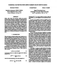
In a first experiment we demonstrate that the method is accurate on synthetic objects with varying degrees of texture (Figure 4). We have simulated the capture setup using a synthetic object texture mapped with two different textures. In each case the concavities of the object were accurately recovered. We have also computed the distance from the recovered displacements to the ground truth displacements (we used ray tracing to recover the ground truth displacements from a triangulated mesh). A color mapped version of this distance on the ground truth is also portrayed in Figure 4. The reconstruction is quite good with an average geometric error is about 0.0327 units on an object of size 2 units (1.6% accuracy). The results of the refinement on two real objects are shown in Figure 5 2 . Notice that in each case the base mesh and the initial displacements (using the method described in Section 4.4.1) are coarse approximations of the true object. After the displacements are refined, the fine scale detail of the 3D geometry becomes apparent. Notice the method performs well on the face sequence, which would be considered hard to capture with traditional methods. The face also exhibits a surface reflectance that deviates from the Lambertian model, but our Lambertian cost function is successful at recovering visually appealing displacements.

=0

pi01 pi11 pi21

pi02 pi12 pi22

for k 6= j

(11)

 pi03 pi13  pi23

(12)

∂ ˆ j )) = ∇Ii (Π(Pi p ˆ j )) · ∇Π(Pi p ˆj ) Ii (Π(Pi p ∂µk   i (p00 dj,x + pi01 dj,y + pi02 dj,z )/w = ∇Ii (pi10 dj,x + pi11 dj,y + pi12 dj,z )/w   u(pi20 dj,x + pi21 dj,y + pi22 dj,z )/w2 − ∇Ii v(pi20 dj,x + pi21 dj,y + pi22 dj,z )/w2 ˆ j . In practice a Gaussian blurred with [u, v, w]> = Pi p version of the image gradient is substituted for ∇Ii . ∂ ∂µk





n j · li |nj |

= =

1 ∂nj · li ∂ 1 + n j · li √ |nj | ∂µk ∂µk nj · nj

(∇µk nj ) · li n j · li − ((∇µk nj ) · nj ) |nj | |nj |3

Recall that: nj =

X

j,k,i∈∆(pj )

7 Conclusions

ˆ j ) × (ˆ ˆj ) (ˆ pk − p pi − p

ˆ j ) = (xk − xj , yk − yj , zk − zj ) and Letting e1 = (ˆ pk − p ˆ j ) = (xi − xj , yi − yj , zi − zj ), e2 = (ˆ pi − p   e1y e2z − e2y e1z e1 × e2 =  −e1x e2z + e2x e1z  e1x e2y − e2x e1y   yk zi − y k zj − y j zi − y i zk + y i zj + y j zk =  −(xk zi − xk zj − xj zi − xi zk + xi zj + xj zk )  xk y i − x k y j − x j y i − x i y k + x i y j + x j y k

We have presented a method for reconstructing the displacements from a base mesh using image data. The method couples the surface normals in the cost function, implying that surface shading cues influence the reconstruction. The experiments validated the effectiveness of this approach on objects with uniform and non-uniform Lambertian surface properties. Experimental evidence also suggests that our method is capable of dealing with slight reflectance deviations from the Lambertian model (e.g., the face example).

Therefore  (yi − yk )dj,z + (zk − zi )dj,y  (zi − zk )dj,x + (xk − xi )dj,z  ∇µ j n j = (xi − xk )dj,y + (yk − yi )dj,x j,k,i∈∆(pj )

2 The

human head data set was obtained by placing the calibration pattern upside down on the subject’s head while the subject rotated on an office chair.

X

6



Figure 4: A synthetic object with different textures used in the experiments. From left to right: an input image, the recovered shaded model, the recovered textured model, and distance to ground truth (dark means close, white means far). The average distance of the recovered displacement to the ground truth was 0.0381 and 0.0274 for the untextured and textured sequences respectively (the size of the whole object is around 2 units). The derivation of ∇µk nj and ∇µi nj are similar. Finally, using the definition of Aj ,Ij and αj from Equations 8 and 9, we have

[2] Neil Birkbeck, Dana Cobzas, Peter Sturm, and Martin Jagersand. Variational shape and reflectance estimation under changing light and viewpoints. In ECCV2006, 2006.

∂αj 1 ∂ = (Aj · Ij ) ∂µk Aj · Aj ∂µk Aj · I j ∂ − (Aj · Aj ) (Aj · Aj )2 ∂µk   ∂ X n j · li ∂ ˆ j )) (Aj · Ij ) = `i + ai Ii (Π(Pi p ∂µk ∂µk i |nj | X ˆ j )) = Ii (Π(Pi p

[3] Yuri Boykov, Olga Veksler, and Ramin Zabih. Fast approximate energy minimization via graph cuts. IEEE Trans. Pattern Anal. Mach. Intell., 23(11):1222–1239, 2001. [4] David Cohen-Steiner, Pierre Alliez, and Mathieu Desbrun. Variational shape approximation. ACM Trans. Graph., 23(3):905–914, 2004. [5] Robert L. Cook. Shade trees. In SIGGRAPH ’84: Proceedings of the 11th annual conference on Computer graphics and interactive techniques, pages 223–231, New York, NY, USA, 1984. ACM Press.

i





   n j · li ∂ ˆ j )) + `i + ai Ii (Π(Pi p |nj | ∂µk  2 X n j · li ∂ ∂ `i (Aj · Aj ) = + ai ∂µk ∂µk i |nj |     X n j · li n j · li ∂ = 2`i `i + ai |nj | ∂µk |nj | i `i

∂ ∂µk

n j · li |nj |



[6] Paul E. Debevec, Camillo J. Taylor, and Jitendra Malik. Modeling and rendering architecture from photographs. In SIGGRAPH, 1996. [7] Y. Duan, L. Yang, H. Qin, and D. Samaras. Shape reconstruction from 3d and 2d data using pde-based deformable surfaces. In ECCV, 2004. [8] O. Faugeras and R. Keriven. Variational principles, surface evolution, pde’s, level set methods and the stereo problem. IEEE Trans. Image Processing, 7(3):336–344, 1998.

References

[9] P. Fua. Reconstructing complex surfaces from multiple stereo views. In ICCV, pages 1078–1085, 1995.

[1] Adam Baumberg, Alex Lyons, and Richard Taylor. 3D S.O.M. - a commercial software solution to 3d scanning. In Vision, Video, and Graphics (VVG’03), pages 41–48, July 2003.

[10] P. Fua and Y. Leclerc. Object-centered surface reconstruction: combining multi-image stereo shading. In Image Understanding Workshop, pages 1097–1120, 1993.

7

Figure 5: The results of the displacement map estimation for a model house made from wood and bark and a human face. From left to right, an input image, the base mesh, the low-resolution starting point (using discrete optimization), two shaded views of the object, and a textured lit rendering of the recovered object. [11] Pau Gargallo and Peter Sturm. Bayesian 3d modeling from images using multiple depth maps. In CVPR, pages 885–891, 2005.

[19] S. Soatto, A. Yezzi, and H. Jin. Tales of shape and radiance in multi-view stereo. In ICCV, 2003. [20] C. Strecha, T. Tuytelaars, and L.J. Van Gool. Dense matching of multiple wide-baseline views. In ICCV, pages 1194–1200, 2003.

[12] C. Hern´andez and F. Schmitt. Silhouette and stereo fusion for 3d object modeling. Computer Vision and Image Understanding, special issue on ’Model-based and imagebased 3D Scene Representation for Interactive Visualization’, 96(3):367–392, December 2004.

[21] George Vogiatzis, Philip Torr, Steve Seitz, and Roberto Cipolla. Reconstructing relief surfaces. In BMVC, 2004. [22] Martin Weber, Andre Blake, and Roberto Cipolla. Towards a complete dense geometric and photometric reconstruction under varying pose and illumination. In BMVC, 2002.

[13] William A. Hoff and Narendra Ahuja. Surfaces from stereo: Integrating feature matching, disparity estimation, and contour detection. IEEE Trans. Pattern Anal. Mach. Intell., 11(2):121–136, 1989.

[23] G. Zeng, S. Paris, L. Quan, and M. Lhuillier. Surface reconstruction by propagating 3d stereo data in multiple 2d images. In ECCV, 2004.

[14] H. Jin, A. Yezzi, and S. Soatto. Stereoscopic shading: Integrating shape cues in a variational framework. In CVPR, pages 169–176, 2000.

[24] Gang Zeng, Sylvain Paris, Long Quan, and Francois Sillion. Progressive surface reconstruction from images using a local prior. In ICCV, pages 1230–1237, 2005.

[15] Jan Kautz and Hans-Peter Seidel. Hardware accelerated displacement mapping for image based rendering. In Proccedings of Graphics interface, pages 61–70, 2001.

[25] L. Zhang, B. Curless, A. Hertzmann, and S. M. Seitz. Shape and motion under varying illumination: Unifying structure from motion, photometric stereo, and multi-view stereo. In ICCV, 2003.

[16] J.-O. Lachaud and A. Montanvert. Deformable meshes with autom. topology changes for coarse-to-fine 3D surface extraction. Medical Im. Anal., 3(2):187–207, 1999. [17] Daniel Scharstein and Richard Szeliski. A taxonomy and evaluation of dense two-frame stereo correspondence algorithms. Int. J. Comput. Vision, 47(1-3):7–42, 2002. [18] Gregory G. Slabaugh, W. Bruce Culbertson, Thomas Malzbender, and Ronald W. Schafer. A survey of methods for volumetric scene reconstruction from photographs. In International Workshop on Volume Graphics, 2001.

8