Object-Oriented Classification of Forest Structure from Light Detection and Ranging Data for Stand Mapping
ABSTRACT
Alicia A. Sullivan, Robert J. McGaughey, Hans-Erik Andersen, and Peter Schiess Stand delineation is an important step in the process of establishing a forest inventory and provides the spatial framework for many forest management decisions. Many methods for extracting forest structure characteristics for stand delineation and other purposes have been researched in the past, primarily focusing on high-resolution imagery and satellite data. High-resolution airborne laser scanning offers new opportunities for evaluating forests and conducting forest inventory. This study investigates the use of information derived from light detection and ranging (LIDAR) data as a potential tool for delineation of forest structure to create stand maps. Delineation methods are developed and tested using data sets collected over the Blue Ridge study site near Olympia, Washington. The methodology developed delineates forest areas using LIDAR data and object-oriented image segmentation and supervised classification. Error matrices indicate classification accuracies with a kappa hat values of 78 and 84% for 1999 and 2003 data sets, respectively. Keywords: LIDAR, light detection and ranging, forest classification, object-oriented image segmentation, supervised classification, stand mapping
F
orest stand delineation is an integral process in forest inventory and forest management. Stands are the primary operational unit at which forest managers make silvicultural decisions and perform financial analysis. The definition of a forest stand varies greatly between disciplines, as well as landowners and their particular operational goals. For this study, stands are viewed from a perspective of active forest management for timber production. A general definition of a stand can therefore be defined as “a community, particularly of trees, possessing sufficient uniformity as regards to composition, age, spatial arrangement, or condition, to be distinguishable from adjacent communities, so forming a silvicultural or management entity.” (Ford-Robertson 1971). Stand delineation has generally been regarded as a subjective process dictated by the needs of the company, agency, or organization that is managing the land (Paine 1981). This research has produced a tool that can assist in delineation of forest stands by providing spatial information about variability in forest structure at a very fine resolution across an entire landscape. This spatial information can then be aggregated based on the needs of the forest landowner into forest stands. Current forest stand delineation techniques generally rely on aerial photography and local knowledge, which can be inconsistent and hard to reproduce (Chubey et al. 2006). The primary advantage of this method is that much of the process is automated, allowing for repeatability and more consistent results. A push toward deriving forest inventory and delineation of stands from remotely sensed data has been investigated for many years. A great body of research is available investigating the use of
various types of imagery to derive forest characteristics. Much of this research focuses on the use of high-resolution imagery to identify individual tree crowns and derive forest inventory information (Gougeon 1995, Brandtberg and Walter 1998, Leckie et al. 2003). The delineation of stands as a secondary step after crown delineation has also been explored with high-resolution imagery (Gougeon 1997, Leckie et al. 2003). Other research with high-resolution imagery has directly addressed the goal of stand delineation (Van Coillie et al. 2006, Warnick et al. 2006). The use of satellite imagery, such as Ikonos-2 and Landsat-TM, for stand characterization has also been explored (Waring and Running 1999, Bergen et al. 2000, Green 2000). However, this research has limited applicability to operational-level processes due to the complexity and costs associated with acquisition and processing of high-resolution imagery. Another technology, airborne light detection and ranging (LIDAR) has recently been intensively investigated for use in forestry applications. Although this type of sensor has been used for terrain mapping applications for many years (Reutebuch et al. 2003), it is still a relatively new tool for forest management. Research into the use of LIDAR for forest management has been investigated extensively in Scandinavia. This research has investigated the use of LIDAR for forest inventory and description of stand level metrics such as basal area, stem density, and volume (Naesset 2004, Magnusson 2006). Other research has been focused on measuring individual tree parameters and producing stand summaries (Naesset and Okland 2002, Andersen 2003, Holmgren and Persson 2004). With the exception of a recent study by Antonarakis et al. (2008),
Manuscript received August 7, 2008; accepted March 30, 2009. Alicia A. Sullivan (
[email protected]), College of Forest Resources, University of Washington, Precision Forestry Cooperative, P.O. Box 352100, Seattle, WA 98125. Robert J. McGaughey, US Forest Service, Pacific Northwest Research Station, Silviculture and Forest Models Team, 400 N 34th St., Suite 201, Seattle, WA 98103. Hans-Erik Andersen, US Forest Service, Pacific Northwest Research Station, Forest and Analysis, 3301 C Street, Suite 200, Anchorage, AK 99503-3954. Peter Schiess, College of Forest Resources, University of Washington, Precision Forestry Cooperative, P.O. Box 352100, Seattle, WA 98195. We thank the Bureau of Land Management for funding of this project, as well as the US Forest Service Pacific Northwest Research Station and Washington State Department of Natural Resources for use of the Blue Ridge study site data. Copyright © 2009 by the Society of American Foresters.
198
WEST. J. APPL. FOR. 24(4) 2009
Table 1. Specifications for light detection and ranging acquisitions at the Blue Ridge study site. Acquisition parameters
1999
2003
Acquisition date Laser scanner Flying height (m) Laser pulse density (pulses/m2) Maximum returns per pulse Platform
March Saab Topeye 200 3.1 4 Helicopter
August Terrapoint ALTMS 900 4.9 4 Fixed-wing aircraft
From Andersen et al. (2005).
Figure 1.
Location of the Blue Ridge study site.
little attention has been given to the use of LIDAR data for land classification. Background Like many forestland owners, the Bureau of Land Management (BLM) in Oregon has recognized the need for more accurate and timely information to meet the goals of its organization. LIDAR shows great potential to assist forest landowners in addressing this need and will become less prohibitive to attain as data acquisition costs decrease. This study was designed for the BLM as a proof of concept research project to investigate the ability of LIDAR-derived data to delineate forest areas. Therefore, the forest classes in the study are intentionally broad; further refinement of the classes will be necessary for each landowner. The method described in this article uses a technique called object-oriented image classification. This is a technique that was developed for classifying images into user-defined classes (Blaschke et al. 2000). This classification method works with image objects (aggregates of pixels) rather than on a pixel-by-pixel basis as used in traditional classification techniques (Chubey et al. 2006). This classification technique was chosen over pixel-by-pixel classification because it incorporates the spatial relation among pixels and their neighbors to segment the image (Camara et al. 1996). Object-oriented image classification has traditionally been performed on bands of spectral information collected by a sensor. In this study, we used LIDAR-derived metrics in place of spectral information as input bands for image segmentation and classification. Although our method requires supervised training to recognize the various classes and some skill in image interpretation, the advantage is automation of much of the manual work reducing the time and effort required to produce a classification of forest structure.
Methods Study Area The area chosen for this research was the Blue Ridge study site located in the Capitol State Forest, west of Olympia, Washington, as shown in Figure 1. LIDAR coverage of the site was obtained in 1999 and 2003. In addition, a series of field plots in the treatment areas were established in 1999 and remeasured in 2003 as part of a longterm silvicultural study, as described in Curtis et al. (2004). The site covers approximately 2 square miles, with a variety of terrain conditions and silvicultural treatments. Stand conditions range from mature to clearcut, along with a large-scale thinning treatment. The
area is representative of many of the managed second growth forests in western Washington and Oregon; a complete description of the Blue Ridge site is available in Curtis et al. (2004). Data Preparation The two LIDAR data sets used in this study were flown in 1999 and 2003 as part of a larger silvicultural study conducted by the Pacific Northwest Research Station of the US Forest Service (Curtis et al. 2004). The specifications for these acquisitions are listed in Table 1. The number of laser returns per square meter is approximately the same for both data sets. The two data sets allow us to investigate the potential to detect changes resulting from management activities or disturbances between two dates. The choice of stand metrics used in this analysis was based on a literature review of forest inventory and photo interpretation manuals. Percentage of canopy cover, stem density, and average height are common forest stand metrics used to delineate forest areas (Spurr 1948, Smelser and Patterson 1975, Franklin 2001). In addition to their use in traditional forest mapping procedures, these parameters were chosen because they can be reliably derived from LIDAR data using the FUSION software package. Although previous studies have shown the potential for using LIDAR intensity and structural information to classify species types (Holmgren and Persson 2004), individual tree species cannot be reliably and consistently derived from LIDAR data sets, and therefore species classification was omitted. Several steps were used to generate the data layers necessary for image segmentation. The raw LIDAR points were processed in FUSION, a LIDAR visualization and analysis program developed by the US Forest Service Pacific Northwest Research Station (McGaughey 2007). To create the percentage of canopy cover raster layer, the raw LIDAR points (georeferenced points collected by the LIDAR sensor) are used with the cover tool in FUSION. This tool calculates the number of LIDAR points above a user-defined height specification and divides by the total number of points in the pixel, resulting in a percentage of cover value for the pixel (McGaughey 2007). The raw LIDAR points along with the bare earth model are then used to create the canopy height model as an input for the canopy maxima tool. The importance of the canopy height model is to remove the effect of terrain on tree height for analysis. The canopy height model is then used in the canopy maxima tool, which identifies the highest LIDAR point in individual crown areas and generates a list of canopy maxima points (McGaughey 2007). Canopy maxima are used to estimate average tree height and stem density on a per-pixel basis. Detailed descriptions of the FUSION tools used in this method can be found in McGaughey (2007). A detailed description of our methodology and workflow are available in Appendix 1 of Sullivan (2008). WEST. J. APPL. FOR. 24(4) 2009
199
Figure 2.
Flow chart of data preparation and analysis.
The results from the data preparation process are raster layers with a pixel size of 29.5 ⫻ 29.5 ft to represent 871.2 ft2, or 1/50th ac. The choice of pixel size was based on the conditions present in the test site and standard conventions for forest inventory. The most important consideration for pixel size in this study was to ensure that the pixel size fell in a range that was large enough to encompass the complete canopy of a mature tree and small enough to detect variation of young stands. The data preparation for input into the image segmentation and classification software is described in Figure 2. Image Segmentation and Classification Object-oriented image classification was performed using SPRING, a program developed by Brazil’s National Institute for Space Research (Camara et al. 1996). The object-oriented image classification method in SPRING uses several steps to accomplish the final classification. First, image segmentation was performed using a region-growing approach, whereby spatially adjacent pixels are grouped to form discrete image objects or regions that are relatively homogeneous in the properties used to define them (Camara et al. 1996). In SPRING, segmentation parameters are set by the analyst and define the value at which adjacent pixels are considered to be different (and therefore not grouped), as well as a minimum object size defined by number of pixels. Once the segmentation is complete, the next step is supervised training of the segmented image. This involves selecting a set of training objects that are representative of each class. In this research, 10 training objects were selected for each class. On the completion of training, the classifier was run with the training objects to classify the rest of the study area. The classifier used in this research is a Battacharya classifier, which is a “distance measure classifier by regions, to measure the statistical separability between a pair of classes” (Camara et al. 1996). The final output from this process is a forest classification map. The classes for this project were determined by the available plot data and silvicultural history for the site. Six stand classes were 200
WEST. J. APPL. FOR. 24(4) 2009
Table 2. Description of stand classes based on study site plot information. Plot values Stand type/class
TPA Min
TPA Max
Mature Thinned Intermediate Young 1 Young 2 Clearcut/road
50 15 355 No data 222 0
210 20 755 No data 533 0
D40 Min
D40 Max
H40 Min
H40 Max
. . . . .(in.) . . . . . . . . . .(ft) . . . . . 26.7 31.2 141.2 152 21.9 24.1 134 150.3 4.6 7.1 45.6 49.2 No data No data No data No data 4.7 4.7 26.75 29.9 0 0 0 0
From Curtis et al. (2004). D40, average diameter of the largest 40 trees per acre; H40, average height of the largest 40 trees per acre; max, maximum; min, minimum; TPA, trees per acre.
identified on the basis of differences in stem density (total number of trees per acre), diameter (average diameter of the largest 40 trees per acre), height (average height of the largest 40 trees per acre), and silvicultural treatment. Species information was not included, as it was not available from LIDAR data at the time of the study. The six stand classes are mature, thinned, intermediate, young 1, young 2, and clearcut/road and are outlined by plot metrics in Table 2. Plot locations were established by survey-grade GPS. Plots that met class descriptions along with aerial photography were used as guides for selecting training objects during the supervised classification. Accuracy Assessment To evaluate the accuracy of the classification results, error matrices were generated for the 1999 and 2003 classifications. From the error matrix, producer accuracy, user accuracy, overall accuracy, and kappa hat (KHAT) were calculated for the classifications (Campbell 2007, Lillesand and Kiefer 2008). The producer accuracy indicates how many pixels of a class were correctly identified by the software and therefore describes the performance of the classifier. The user
Table 3.
Blue Ridge stand classification error matrices. Visual Classification
Spring classification
Mature
Thinned
Intermediate
1999 Classification error matrix and classification accuracies Mature 196 0 0 Thinned 16 27 2 Intermediate 5 0 66 Young 1 0 0 0 Young 2 0 0 14 Clearcut/road 4 5 1 Column total 221 32 83 Overall accuracy KHAT KHAT variance 2003 Classification error matrix and classification accuracies Mature 215 0 0 Thinned 2 16 0 Intermediate 11 0 62 Young 1 0 0 0 Young 2 2 0 3 Clearcut/road 4 8 0 Column total 234 24 65 Overall accuracy KHAT KHAT variance
Young 1
Young 2
Clearcut/road
Row total
Producers (%)
0 0 0 17 5 2 24
0 0 0 19 43 3 65
0 0 1 1 2 62 66
196 45 72 37 64 77 491
88.69 84.38 79.52 70.83 66.15 93.94
Users 100.00% 60.00% 91.67% 45.95% 67.19% 80.52% 83.71% 78.20% 0.0001088
0 0 0 13 5 4 22
0 0 2 7 52 0 61
0 0 0 5 0 68 73
215 18 75 25 62 84 479
91.88 66.67 95.38 59.09 85.25 93.15
100.00% 88.89% 82.67% 52.00% 83.87% 80.95% 88.49% 84.46% 0.0000878
Boldface numbers show the number of correctly classified pixels in both the Spring Classification and Visual Classification in each dataset. KHAT, kappa hat.
accuracy describes the accuracy users could expect if they went to a pixel of that classification on the ground. Overall accuracy reports the overall accuracy of the individual classification across all of the classes. To standardize the accuracy assessment between the two data sets, KHAT was calculated for each of the dates. This KHAT is an estimate of the kappa value and is a measure of agreement based on the difference between the actual agreement in the error matrix and the chance agreement (Congalton and Green 1999). It also allows for comparison of the overall accuracy between different classifications and is a useful tool for evaluating results across dates (Congalton and Green 1999, Lillesand and Kiefer 2008). Classification accuracy was assessed using a subsample of the classified pixels. A uniform grid of 600 points was generated through the Hawth’s Tools extension (Beyer 2004) in ArcMap at a spacing of 246 ⫻ 246 ft. This grid was overlaid on the classified images; pixels that contained points from the grid were evaluated for accuracy of classification by visual inspection of aerial photography and comparison to plot data where available. Any pixel with more than one structural classification was not considered in the accuracy assessment.
Results and Discussion Classification Accuracy The accuracy assessments show promising results for the method developed in this research. Landis and Koch (1977) characterize KHAT values greater than 80% as representing strong agreement and KHAT values between 40 and 80% as having moderate agreement. The KHAT value for 1999 is 78.20%, and the KHAT value for 2003 is 84.46%; these values represent a moderate agreement for 1999 and a strong agreement for 2003. The error matrices for the two dates depict the results of the accuracy assessment and also provide insight into confusion between classes. In both 1999 and 2003, the greatest amount of confusion occurred between the young 1 and young 2 classifications. The resulting low values for producer accuracy and user accuracy in these classes reflect this. The confusion between the young 1 and
young 2 most likely results from the similarity between the classes and the lack of plot data in the young 1 category to refine the class descriptions. The error matrix results for the thinned and clearcut/road classifications also reflect a fair amount of confusion. The accuracies of these classes are affected in both dates. The error matrices and classification accuracies by date are shown in Table 3. A z-statistic was calculated for both dates to test whether the classifications were significantly different from a random classification. The test used the KHAT value and the variance of the KHAT value for each classification to calculate the z-statistic (Congalton and Green 1999). Both classifications were tested at the 95% confidence level, with degrees of freedom assumed to be infinite and a critical value of 1.96 (Congalton and Green 1999). The 1999 classification had a z-value of 74.96 and the 2003 classification had a z-value of 90.13. Both z-values are highly significant, so both classifications are significantly different from a random classification. The intended application of this method is to generate stand type maps from the classification results for use in forest management. Therefore, the user accuracy will have the most impact on the quality and usefulness of the final product. In both classifications, there are specific classes with low user accuracies that are influenced by confusion between classifications and conditions present in the study area. For example, the relatively low user accuracy associated with the thinned class in the 1999 classification may be attributed to confusion with open areas within a mature stand. This confusion is apparent from the error matrix, as the greatest numbers of misclassified pixels in the thinned class were classified as mature in the visual classification, whereas at the pixel level, there is a gap or an obvious lower density of trees, so the surrounding stand is mature and was visually classified as such. In the case of the 2003 data, low user accuracy occurs in the young 1 class. In this case, areas on the edges of clear cuts were classified as young 1 because of the presence of brush and opportunistic vegetation entering these areas. Another area of confusion that affects the user accuracy of the young 1 class are areas of lower density, brush, or gaps in the young 2 stands that are classified as WEST. J. APPL. FOR. 24(4) 2009
201
Figure 3. Study area and classification results. (A) 1999 ortho photograph of the Blue Ridge study site. (B) stand map from the 1999 light detection and ranging (LIDAR) data. (C) stand map from the 2003 LIDAR data. The circled areas in C highlight the areas of operational activities between acquisitions detected in the 2003 classification. Heavy black lines in B and C represent possible stand boundaries based on the classifications.
202
WEST. J. APPL. FOR. 24(4) 2009
young 1. This may also represent areas of high seedling mortality due to poor planting techniques, overtopping by brush, or animal browse. This high level of confusion between the young 1 and young 2 classes may also suggest that these classes are too similar and that class definitions may need to be refined in a future study. In both cases, the aggregation of the smaller classification patches into the larger stand type may decrease the error associated with these misclassifications. The process of aggregating these smaller areas will be dependent on the analyst and the desired level of detail for the final stand map. An advantage of this method is that is does provide a great level of detail that can then be summarized into operational forest stands. Stand Classification As shown in the previous section, this method has produced moderate to highly accurate classification results. To produce stand maps, additional interpretation by an analyst may be required to meet the desired goals of the landowner. The classification maps are the final output from the segmentation and classification process. The results from the classifications are shown in Figure 3. Each class is uniquely colored and demonstrates the scale of detail possible from this method. Figure 3A is the 1999 orthorectified photograph of the study site, Figure 3B is the 1999 classification map, and Figure 3C is the 2003 classification map. As a final exercise for this project, potential forest stands were manually delineated from the classification maps. Multiple stand configurations would be possible from these classification results; therefore, the accuracy of the suggested stands was not examined. In Figure 3B and 3C, heavy black lines depict the potential stand boundaries. In some cases, stands represent the aggregation of several small regions based on object size and spatial position. Although an extra step is required to create operational stands, creation of them also provides a great benefit. The ability of the method to detect small differences within a stand may provide important information about small scale disturbances or detection of management activities. An example of this is given by red circles in Figure 3C showing a new harvest unit and road. The fine level of detail also allows for great flexibility and multiple stand delineations from one classification.
Conclusions The current study has shown that delineation of forest structure is possible from LIDAR data using object-oriented image segmentation and supervised classification. It has also been shown that a high level of structural variability, as well as operational activities such as road construction, can be detected. This method provides a tool for forest landowners with LIDAR coverage to automate delineation of forested landscapes into user-defined classes that can then be used as the basis for products such as stand maps. These classification maps provide another available product from the investment of LIDAR acquisition. In addition, this method uses free software packages (FUSION, SPRING) for the processing and analysis, reducing additional costs. The primary limitation of this research is the current cost of LIDAR data acquisition and processing. However, prices per acre of data acquisition continue to decrease, and organizations such as the Puget Sound LIDAR Consortium (Puget Sound LIDAR Consortium 2008) have begun providing access to LIDAR data at no charge to the public. Another limitation is the requirement to define the desired level of spatial detail and appropriate classification classes for
each landscape or study area. To improve on this technique, a variety of forest ecosystems, pixel sizes, and owner-specific classification classes should be investigated. As research into the application of LIDAR for forest management continues, new techniques for deriving information will be developed, and these new information layers may provide valuable information in the classification process. Information about species, diameter, crown height, and crown width may assist in distinguishing between the classes that are currently being confused during classification. The addition of high-resolution imagery to the classified results may also prove very useful for delineation of forest stands. Finally, investigation of the use of commercial image segmentation and classification software may provide greater accuracy in classification due to additional functionality to perform hierarchical classifications.
Literature Cited ANDERSEN, H.-E. 2003. Estimation of critical forest structure metrics through the spatial analysis of airborne laser scanner data. PhD dissertation, Univ. of Washington, Seattle, WA. ANDERSEN, H.-E., R.J. MCGAUGHEY, AND S.E. REUTEBUCH. 2005. Forest measurement and monitoring using high-resolution airborne LIDAR. In Productivity of Western Forests: A Forest Products Focus. Harrington, C.A., and S.H. Schoenholtz (eds.). US For. Serv. Pacific Northwest Res. Stn., Portland, OR. ANTONARAKIS, A.S., K.S. RICHARDS, AND J. BRASINGTON. 2008. Object-based land cover classification using airborne LIDAR. Remote Sens. Environ. 112(6): 2988 –2998. BERGEN, K., J. COLWELL, AND F. SAPIO. 2000. Remote sensing and forestry: Collaborative implementation for a new century of forest information solutions, J. For. 98(6):4 –9. BEYER, H.L. 2004. Hawth’s analysis tools for ArcGIS. Available online at www. spatialecology.com/htools; last accessed Feb. 15, 2008. BLASCHKE, T., S. LANG, E. LORUP, J. STROBL, AND P. ZEIL. 2000. Object-oriented image processing in an integrated GIS/remote sensing environment and perspectives for environmental applications. Umweltinformation Fu¨r Planung, ¨ ffentlichkeit/Environ. Inform. Plann. Politics Public 2:555–570. Politik Und O BRANDTBERG, T., AND F. WALTER. 1998. Automated delineation of individual tree crowns in high spatial resolution aerial images by multiple-scale analysis. Machine Vis. Appl. 11:64 –73. CAMARA, G., R.C.M. SOUZA, U.M. FREITAS, AND J. GARRIDO. 1996. SPRING: Integrating remote sensing and GIS by object-oriented data modeling. Comput. Graph. 20(3):395– 403. CAMPBELL, J.B. 2007. Introduction to remote sensing. Guildford Press, New York. 622 p. CHUBEY, M.S., S.E. FRANKLIN, AND M.A. WULDER. 2006. Object based analysis of Ikonos-2 imagery for extraction of forest inventory parameters. Photogramm. Eng. Remote Sens. 72(4):383–394. CONGALTON, R.G., AND K. GREEN. 1999. Assessing accuracy of remotely sensed data: Principles and practices. Lewis Publications, Boca Raton, FL. 137 p. CURTIS, R.O., D.D. MARSHALL, AND D.S. DEBELL. 2004. Silvicultural options for young-growth Douglas-fir forests the Capitol Forest study—Establishment and first results. US For. Serv. Gen. Tech. Rep. PNW-GTR-598. FORD-ROBERTSON, F.C. 1971. Terminology of forest science, technology, practice and products. The multilingual forest terminology, series 1. Society of American Foresters, Washington, DC. FRANKLIN, S.E. 2001. Remote sensing for sustainable forest management. Lewis Publications, Boca Raton, FL. 407 p. GOUGEON, F.A. 1995. A crown-following approach to the automatic delineation of individual tree crowns in high spatial resolution aerial images. Can. J. Remote Sens. 21(3):274 –284. GOUGEON, F.A. 1997. Recognizing the forest from the trees: individual tree crown delineation, classification and regrouping for inventory purposes. P. 807– 814 in Proc. third international airborne remote sensing conference and exhibition, vol. II. Copenhagen, Denmark, July 7–10, 1997. GREEN, K. 2000. Selecting and interpreting high-resolution images, J. For. 98(6):37–39. HOLMGREN, J., AND Å. PERSSON. 2004. Identifying species of individual trees using Airborne Laser Scanner. Remote Sens. Environ. 90(4):415– 423. LANDIS, J., AND G. KOCH. 1977. The measurement of observer agreement for categorical data. Biometrics 33:159 –174. LECKIE, D., F. GOUGEON, N. WALSWORTH, AND D. PARADINE. 2003. Stand delineation and composition estimation using semi-automated individual tree crown analysis. Remote Sens. Environ. 85:355–369. WEST. J. APPL. FOR. 24(4) 2009
203
LILLESAND, T.M., AND R.W. KIEFER. 2008. Remote sensing and image interpretation. John Wiley & Sons, Hoboken, NJ. 750 p. MAGNUSSON, M. 2006. Evaluation of remote sensing techniques for estimation of forest variables at stand level. PhD dissertation, Swedish Univ. of Agricultural Sciences, Umeå, Sweden. MCGAUGHEY, R.J. 2007. FUSION/LDV: Software for LIDAR data analysis and visualization. Electronic manual. US For. Serv. Available online at www.fs.fed.us/eng/rsac/fusion; last accessed June 29, 2008. NAESSET, E. 2004. Practical large-scale forest stand inventory using small-footprint airborne scanning laser. Scand. J. For. Res. 19(2):164 –179. NAESSET, E., AND T. OKLAND. 2002. Estimating tree height and tree crown properties using airborne scanning laser in boreal nature reserve. Remote Sens. Environ. 79:105–115. PAINE, D.P. 1981. Aerial photography and image interpretation for resource management. John Wiley & Sons, New York. PUGET SOUND LIDAR CONSORTIUM. 2008. Puget Sound Lidar Consortium: Public-domain high-resolution topography for western Washington. Available online at pugetsoundlidar.ess.washington.edu; last accessed Aug. 1, 2008. REUTEBUCH, S.E., R.J. MCGAUGHEY, H.-E. ANDERSEN, AND W.W. CARSON. 2003. Accuracy of high resolution LIDAR terrain model under a conifer forest canopy. Can. J. Remote Sens. 29(5):527–535.
204
WEST. J. APPL. FOR. 24(4) 2009
SMELSER, R.L., JR., AND A.W. PATTERSON. 1975. Photo interpretation guide for forest resource inventories. US Forest Service and National Aeronautics and Space Administration, Houston, TX. SPURR, S.H. 1948. Aerial photographs in forestry. Ronald Press Company, New York. SULLIVAN, A.A. 2008. LIDAR based forest stand delineation. M.Sc. thesis. University of Washington, Seattle, WA. VAN COILLIE, F.M.B., L.P.C. VERBEKE, AND R.R. DE WULF. 2006. Semi-automated forest stand delineation using wavelet-based segmentation of very high resolution optical imagery in Flanders, Belgium. In Proc. of 1st International conference on object-based image analysis (OBIA 2006). Lang, S., T. Blasche, and E. Scho¨pfer (Eds.). Available online at www.commission4.isprs.org/obia06/papers.htm; last accessed Aug. 2009. WARING, R.H., AND S.W. RUNNING. 1999. Remote sensing requirements to drive ecosystem models at the landscape and regional scale. P. 23–37 in Integrating hydrology, ecosystem dynamics, and biogeochemistry in complex landscapes. Tenhunen, J.D., and P. Kabat (eds.). John Wiley & Sons, New York. WARNICK, R.M., K. BREWER, M. FINCO, K. MEGOWN, B. SCHWIND, R. WARBINGTON, AND J. BARBER. 2006. Texture metric comparison of manual forest stand delineation and image segmentation. In Proc. of Eleventh biennial Forest Service remote sensing applications conference. April 24 –28, 2006. Salt Lake City, UT.