1
Object-oriented Implementation of a Constraint based geometric Modeling Manfred Rosendahl, University Koblenz, Institute for Computer-Science,
[email protected] Problem considered Modelling in CAD-applications demands to define not only the geometric objects, but rather also to define the functional dependences between the geometric objects and/or between other variables as dimensions or material constants. This is done with the help of Constraints. By this we can demand that the distance of 2 points should have a changeable dimension or that 2 lines are of equal length or have to be parallel. The technologies to the solution of these geometric Constraint systems can be divided in 3 classes: • Equation based methods. Here the Constraints are represented through non linear equations between the variables [Light, Gossard 1982]. • Rule bases methods. Here geometric reasoning mechanism in which the dimensions and geometric relationships are defined as either facts or rules are used [Verroust, Schonek, Roller, 1992] • Graph based methods In the Graph based technologies the Constraints are modelled as Hyper-edges between the points or other variables. Instead to use a Hyper- graph, one can work also with a bipartite graph, in which Variables and Constraints respectively are initially connected by not oriented edges. Depending on the number of Constraints, out of a given subset of the variables, the remaining variables can be calculated. The specific type of modelling makes it possible to use constructive operations, when evaluating the graph from any sufficient set of given variables. Therefore it is possible to select after the creation of the model, which variables are free and which are calculated. Not only a point can be calculated as an intersection by 2 lines, but rather if moving the intersection point, the lines appropriately move. To construct out of the model and the fixed variables a calculation sequence an analysis of the degrees of freedom (DOF) is used. The goal is to produce out of the non oriented Constraintgraph an oriented graph. If a sequential calculation is possible, an acyclic graph should result. In many cases where cyclic dependences exist, however only a graph with one or more cycles can be produced. If too many variables are fixed, the system is over constrained, and then no orientation is possible. Work in this direction is done by [Berling, 1996], [Fudos, Hoffmann, 1993], [Hsu, Brüderlin, 1997]. Results obtained The following paper work extends the approach of [Berling, 1996]. Richer classes of constraints are regarded. Furthermore it is considered in the analysis of the degree of freedom that many Constraints are not independent of one another. So a point in the 2D will have 2 degrees of freedom, but it is not possible to have 2 Constraints, which influence in only the X or only the Y coordinate. Furthermore the locus given by the Constraints may not be defined by 2 circles with the same midpoint or by 2 parallel lines. A goal was also that strongly underdetermined systems show a meaningful behavior. Therefore Constraints have effects not only on the directly adjacent points, but rather they are propagated onto indirectly connected points. Finally for some frequently occurring configurations, which have cycles and can normally only be solved by an equation system, with its well known problems, direct solutions are given. The methods described in this paper are implemented and used for an intelligent diagram editor (KOGGE= KOblenz Graph GEnerator). Geometric Modeling In the creation of a geometric 2D-Modells, one has per point 2 degrees of freedom and 1 degree of freedom per Scalar-value as for example the radius of a circle. These degrees of freedom are restricted by the Constraints to be fulfilled. The Constraint, distance of 2 points, reduces 1 degree of freedom. A construction can fulfill therefore maximally so many Constraints as degrees of freedom are available.
2
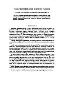
Furthermore one must consider that many Constraints influence position of the points among one another and other constraints influence the position and alignment of the total construction. So the distance of 2 points and the Constraint that demands, that 3 points form a right angle, only influence the position of the points to one another. For the relative position of the points, that is the congruent form; n points have only 2n-3 degrees of freedom. Therefore in a triangle, in which 3 side lengths are fixed, one cannot fix another angle. The points, Scalar variables and Constraint are the nodes of a bipartite graph. The points and the scalar variables make one class (this class is named in the following the variables), and the other class make the Constraints. The edges represent the relations between the Constraints and the variables. Example: 2 Points with distance and horizontal alignment: Horizontal P1
P2 Distance d
Figure 1 The variables are connected later in the arranged graph with maximally so many incoming edges as they have degrees of freedom. If the value of the variables is fixed, then the adjacent edges are oriented as out-going. If a scalar variable is used for several Constraints, only one edge can be oriented as incoming. The Constraint nodes have an edge connection to each variable, which is influenced by then. In the literature in most cases Constraints are considered, which bind a fix number of degrees of freedom. A Constraint, which determines the distance from 2 points, is connected to 2 points and 1 scalar value. Both the two points determine the distance or the distance and one point specify a locus for the other point. It is said then that the distance Constraint consumes 1 degree of freedom. In the modeling regarded here, some Constraints have a varying number of adjacent variables; therefore the Constraints have a given degree of freedom. The Constraint distance has 2 degrees of freedom; therefore 2 of the adjacent edges are oriented as incoming. This could by again: • Both points: Then the distance is fixed. • 1 Point and the distance d: Then for the other point a locus is fixed, here it is a circle with the first point as center and the distance d as radius. A Constraint consumes so many degrees of freedom of the variables, as it has out-going edges, (number of adjacent edges - degree of freedom). The Constraint horizontal for example specifies that all points on a set have the same Y-coordinate. One edge can be oriented incoming. The adjacent point determines the Y-coordinate of the other points. The same applies for the Constraint circle. Beside center and radius still a number of points, which are positioned on the circle, are adjacent to the constraint circle. Now either by 3 Points on the circle the center and the radius are fixed, or the center and the radius determine a locus for the points on the circle. Also all other combinations are possible, e.g. 2 points on the circle and the radius determines the center. In order to solve all cases for the different constraints, each constraint-class has a method compute, which determines for all adjacent variables, with out going edges, the value and/or a locus. During the evaluation, according to the fixed variables, out of the non- oriented graph an oriented graph is produced. This graph is, if possible, evaluated in the sequence of the topological order. It is however not always possible to orient the graph cycle-free. Then in the graph the strong components are computed. That is a partitioning of the node-set in subsets with the property that the cycles are all within the strong components. The strong components with more than one node are computed in general by iteration. This does not lead however always to a result. Therefore later in this paper procedures are introduced, which permit a direct solution for some frequently occurring cases. The computation of the strong components can be done according to the topological sorting. Description of some the Constraints
Thorizontal
Degree of freedom 1
Adjacent nodes Points,
which
Description are
One point determines the Y-
Fixed Coordinate Y
3
aligned horizontal Points, which are aligned vertical 2 points und one Scalar
Tvertical
1
Tdistance
2
Tangle
2
2 or more points and a scalar
Tangle3P
3
3 points and one scalar
Tcircle
3
Radius, 2 edges to the Center and further points on the circle
Tline
2
2 or more points, which are collinear
Tdistancelp
3
Tarc
3
Scalar (distance) und 2 Points, which define a straight line and one point, which distance is determined Radius, 2 edges to the center, starting point, endpoint of the arc and other points on the arc.
Toperator
2
2 Scalars as operands und one Scalar as result
Coordinate of the other points One point determines the XCoordinate of the other points 2 points determine a distance or the distance and one point determine a locus of the other point 2 points determine a angle or an angle and one point determine a locus for the other points 3 points determine a angle build by them or an angle and 2 points determine a locus for the third point The circle is fixed by 3 incoming edges. The outgoing edges determine the radius or locus for the center resp. for points on the circle. 2 incoming edges determine the straight line on which all points are positioned. The outgoing edges determine the locus for the other points. 3 points determine the distance or the distance and 2 points determine the 3. point
The circle is determined by 3 incoming edges. The outgoing edges determine the radius or locus for the center resp. for points on the circle. The operands determine the result or the result and one operand determine the other operand.
X XY
XY
XY
XY
XY
XY
XY
XY
Other Constraints can be built up from these. The constraint that 2 lines have same length is defined by 2 distance constraints, whose distance- value is unified. (Figure 2)
Figure 2
Figure 3
Similar 2 parallel lines can be defined (Figure 3)
4
An intersection-point can be defined by two line Constraints (Figure 4).
Figure 4 The intersection must be on the line of the points 1-2 and the line of the points 3-4. If the intersection is moved, then the points 1 and 4 move, since 2 and 3 are fixed. The orientation of the graph is then according to Figure 5. When moving the points 1-4 the intersection point is moved similarly.
Figure 5 Also a line, which goes from one point tangential to a circle, can be defined by a circle and a right-angle. Since the center of the circle fixes 2 degrees of freedom of the circle constraint and because only one edge between 2 nodes in the graph is allowed, sub-nodes must be inserted between the center-point and circleconstraint. To keep the graph bipartite, a Constraint node and a variable node must be inserted (Figure 6).
Figure 6
5
If 2 circles have to touch themselves tangential, then this can be defined by the distance of the center points. The distance must result in the sum and/or the difference of the radii. By appropriate orienting of the graph with a change of the radii the new centers can be computed, but also with a change of the centers new radii can be computed. The construction has altogether 7 degrees of freedom (2 points, 2 radii and a distance). In this case the circle-Constraint does not bind a degree of freedom, since it has 3 degrees of freedom and also only 3 adjacent variables. The distance-constraint has 2 degrees of freedom and 3 adjacent edges, though it binds one degree of freedom. To the sum the same applies. Altogether thus 5 degrees of freedom remain. They could be fixed by: • The coordinate of one center, 2 radii and the direction of the other center • The coordinates of 2 center-points and one radius. If an arc should connect tangential to a line, then the end point of the line and the starting point of the arc must be coincident, furthermore it must be tangential, i.e. the two points of line and the center point of the circle form a right angle (Figure 7).
Figure 7 Orientation of the Constraint graph The degree of freedom of the variables is reduced by incoming edges. If the degree of freedom is reduced to 0, all further edges must be oriented as outgoing edges. As shown some constraint affects however only the X and/or Y coordinate of a point. Therefore the degree of freedom cannot be simply down-counted, but the following transit ion matrix must be used:
Figure 8 A point has initially 2 degrees of freedom, which corresponds to the state isnot. If the x-coordinate is fixed by a Constraint, the state changes into isx. Now it can only fulfill yet another Constraint, which changes also the Y-coordinate. This can be either a Constraint, only affecting the Y-coordinate (isy) or a Constraint, which specifies a locus (isxy). Altogether one point can fulfill the following Constraint pairs: • Isx, isy • Isx, isxy • Isy, isxy • Isxy, isxy
6
Also the function, which for one point computes the still existing degrees of freedom, has a parameter, which specifies what additionally should be fixed. If it is possible to orient a Constraint graph cycle-free this orientation can be also found. A possible cycle-free orientation however cannot be computed always. Example: 3 points are given, which are connected by 2 lines with a distance constraint each (Figure 9).
Figure 9 If point 3 is moved so far that its distance from the point 1 is larger than the sum of the distances, one will find no more solution for the point 2. If the point 1 is not fixed, the moving of point 3 must be propagated to point 1, so that point 1 is pulled tight accordingly. The oriented Constraint graph then has the following form:
Figure 10 For the point 2 there is then only the locus circle around 3 with radius d2. From the current position of point 2 a perpendicular to this circle is placed. The same is done at point 1. If point 3 is shifted, the points 2 and 1 are pulled tight, whereby the arrangement approaches ever more a straight line. Algorithm to Orient the Constraint graph Before it is tried to orient the non directional graphs, first it is tested whether the construction is not overconstrained. For the individual Constraints it must be examined whether they determine the form, the position or the adjustment. The Constraints tdistance, tangle3p, tdistancelp reduce always the form degree of freedom by one, if its value is given, and/or if the same value was already used in another Constraint. Trightangle reduces the form degree of freedom by one, whereas tline reduces it by the number of points-2. The Constraints tcircle and tarc reduce the form degree of freedom for each point, which must be on the circle. With the Constraints thorizontal, tvertical, tangle the first Constraint and the first two points determine the adjustment, all further points and all further Constraints reduce the form degree of freedom. The first fixed point determines the position of the construction. Further fixing of points reduces the form degree of freedom. Furthermore fixing of points and further Constraints, e.g. distances, can lead to dependencies, which can make the construction even over-constrained. To the distances between points applies:
dx(P1-P2) , dx(P2-P3) -> dx(P1,P3) dy(P1-P2) , dy(P2-P3) -> dy(P1,P3) dx(P1-P2) , dy(P1,P2) -> d(P1,P2) If points are fixed:
Fixx(P1) , Fixx(P2) -> dx(P1,P2) Fixy(P1) , Fixy(P2) -> dy(P1,P2) Fixx(P1),Fixy(P1),Fixx(P2),Fixy(P2)-> d(P1,P2) These conditions are proved by matrices
7
Md[n,m]=true Mdx[n,m]=true Mdy[n,m]=true Fixx[n]=true Fixy[n]=true
d(Pn,Pm) fixed dx(Pn,Pm) fixed dy(Pn,Pm) fixed x Coordinate of Pn fixed y Coordinate of Pn fixed
For Mdx und Mdy the hull is constructed
Md := Md + Mdx*Mdy Fixx[n] and Fixx[m] -> Mdx[n,m]=true Fixy[n] and Fixy[m] -> Mdy[n,m]=true Fixx[n] and Fixy[n] and Fixx[m] and Fixy[m] -> Md[n,m]=true If the appropriate position is already set in the matrix, the construction is over-constrained. Finally it must be examined whether Constraints of angle between 3 points (trightangle or tangle3p) form a closed polygon with n points. Then the construction is over-constrained, because in a closed polygon of n points there are only n-1 independent angles. If the analysis of the degree of freedom does not result in the fact that the construction is over-constrained it is searched for an orientation of the graph, which is as cycle-free as possible. If the graph can be oriented cycle-free, this orientation is used later. If there still remain non directed edges, or if the solution contains cycles, the solution with the minimum number a cycles is searched for. There are 2 methods: 1. Method: Matching expansion If an edge cannot be oriented, then no degree of freedom is still available at both adjacent nodes. In order to orient the edge, thus an incoming edge must be transformed into an outgoing at an adjacent node. However a third node, which is adjacent with this edge, must have still another degree of freedom available. If this is not the case, one must change an edge direction in this node also. This is repeated until one reaches to a node with a still existing degree of freedom, or to a node which was already on the way. If a node with a degree of freedom is found, all edges on the way are reoriented; otherwise the search is broken off. This search, which is known also as the determination of a maximum Matching in bipartite graph (McHugh, 1990, side 200ff), is realized by a recursive function search. If at all adjacent nodes, which are still connected by non oriented edges, no way to a node with a remaining degree of freedom is found, the Constraint system is over-constrained and no solution exists. 2. Method: Brute Force: Systematically all possible orientations are examined, and the solution is selected, which has the fewest number of nodes on a cycle. By previous examination of the degrees of freedom the case that no solution exists, and thus to in any case the whole solution tree must be traversed, is excluded. Evaluating the Constraint- Graph The graph received after the orientation, now can contain still cycles. Therefore first the strong components are determined. Here nodes between a cycle exists are combined into a component. If the graph does not have cycles each component exists of exactly one node. The determination of the strong components is done by a recursive depth-first- search. The graph of the strong components forms a DAG. Therefore the strong components can be evaluated in the order of the topological sorting. The evaluation of a strong component with more than one node is not sequentially possible. Here an iterative method can be used. However a set of equations does not have to be solved over all nodes in the strong component. Rather a set of variables V is determined, which dominates all cycles of the component. This is called the feedback Vertex set F. It is searched for a minimal set F. During the iteration the nodes of F are computed in a loop in the order of the topological sorting. Thereby if another node from F or the same node is used, the old value is taken. This is made until the values of the nodes of F do not change or a maximum number of runs is reached. If the evaluation for the total graph is not successful, first the longest cycle in the oriented graph is determined. On this circle all edges are turned. Thereby the number of incoming and outgoing edges remains the same for each node. To the in such a way changed graph the same procedure is applied. During the evaluation of the cycle-free graph of the strong components, each component, which has only one node, is computed after all nodes, from which edges are incoming. To do this the method compute is called for the node.
8
With the variable-nodes (tv and tnod) we will proceed as follows: tv.compute: no action. The value is already computed by the Constraint node connected with an incoming edge. Tnod.compute: By the Constraint nodes connected with an incoming edge maximally 2 loci are fixed for the point node. This can be: • X-coordinate • Y-coordinate • Line • Circle A function computexy computes the new coordinates from the past coordinates and the demanded loci, if this is possible. The computation cannot be possible e.g., if a circle does not have an intersection with the other locus. If there is one locus for one point only, the perpendicular line is constructed from the past position on this circle and/or this line.
Figure 11 For each class of the Constraint nodes exists a special method. These methods are to be described for some classes: Thorizontal: The node has an incoming edge. Y coordinate of this point determines the Y coordinate of the other points. Tline: The 2 points at the incoming edges, determine the Hessian standard format (A, B, C) of the defined line. This line defines for the points of the out going edges a locus. Tdistance: This node has 3 adjacent variable nodes. The value node contains the distance of the two point nodes. If the value node is outgoing, then out of the two points the distance is computed. This is called a steered measure. The value of the measure is adjusted each time the points change. If the value is incoming, it determines together with one point a circle, as the locus for the other point. Then it is called a steering measure. Tangle3P: This node has 4 adjacent variable nodes. The value node contains the angle, which is spanned by the 3 point nodes. If the value node is outgoing, from the 3 points of the angles is computed. If it is incoming, it determines together with two points a locus for the third point. Tdistancelp: This node has 4 adjacent variable nodes. The value node contains the distance of the line, made by 2 points, and the third point. If the value node is outgoing, from the 3 points the distance is computed. If it is incoming, it determines with two points a locus for the other point. Tcircle: If the points, which must be positioned on the circle, are all connected by outgoing edges, center and radius of the circle define a locus for the points on the circle. If 3 points are connected by incoming edges, center (2x) and radius must by oriented as outgoing. The center and the radius are computed from the 3 points. If 1 or 2 points of the circle are oriented as incoming, for the radius and/or the center point a locus is given. Direct solutions for some configuration with cycles If there is a cycle, the iteration frequently does not converge. Therefore for some frequently occurring cases a direct solution defined.
1. Circle and its center point (Figure 12) The Circle (3 DOG) is given by: • A locus for the center point • A point an the circle • The radius. The second locus for the center is given by the circle. This situation can be computed directly.
9
Figure 12
2. Angle-chain E.g. the distance D-E is changed: The angle relation between D-E-A does not change. Therefore the locus for the line from E to A can be computed directly.
Figure 13
3. Rigid A figure is called a rigid, if its form is fixed. Form a set of nodes a Rigid, they can be shifted or turned only as a whole. Example: Moving E
Figure 14 Cycles: E, D form a Rigid C, B, A must not change their form = > A, B, C, D, E can only turned around X together.
10
4. Temporarily removing the fixing of points
Figure 15 The distance of DE is to be changed. If the fixing of A is removed an orientation can be found. After the computation all points are shifted by a vector in such a way that A gets its old position. If two points are fixed, then between them a new distance Constraint is introduced. After the computation the figure must be turned and shifted in such a way that both points get the old position. In this case there may not be a Constraint, which fixes a direction. Literature [Berling96] Berling R. 'Eine Constraint-basierte Modellierung für Geometrische Objekte', Dissertation. [Fudos, Hoffman, 1993] I. Fudos and C. M. Hoffmann. Correctness proof of a geometric constraint solver. Technical Report 93-076, Purdue University, Computer Science, 1993. [Hsu, Brüderlin 1997] C. Hsu, B. Brüderlin. "A Hybrid Constraint Solver Using Exact and Iterative Geometric Constructions," in CAD Systems Development -- Tools and Methods, D. Roller, P. Brunet, eds., Springer Verlag, 1997. [Kondo, 1992] K. Kondo. Algebraic method for manipulation of dimensional relationships in geometric models. Computer Aided Design, 24(3):141--147, March 1992. [Light, Gossard 1982] R. Light and D. Gossard. Modification of geometric models through variational geometry. Computer Aided Design, 14:209--214, July 1982 [McHugh 1990] McHugh J., ‘Algorithmic Graph Theory’, Prentice-Hall, New Jersey 1990. [Verroust, Schonek, Roller, 1992] A. Verroust, F. Schonek, and D. Roller. Rule-oriented method for parameterized Computer-aided design. Computer Aided Design, 24 (10):531-540, October 1992.