Field Recovery and Error Estimation in FEM ... The computational intensive parts of such programs, ... Object-oriented programming techniques have therefore.
Object-Oriented Implementation of Field Recovery and Error Estimation in FEM Knut Morten OKSTAD and Trond KVAMSDAL SINTEF Applied Mathematics, N{7034 Trondheim, Norway 1. INTRODUCTION Computer programs for numerical solution of partial di�erential equations are traditionally coded in the FORTRAN programming language. The computational intensive parts of such programs, either they are based on the nite element (FE) method or some other numerical procedure, consist mainly of various vector and matrix operations. FORTRAN has therefore been regarded as the best computer language for implementing these programs since it is particularly suitable for manipulation of large arrays. However, as the computers of today become more and more powerful and the compilers more and more e�cient, the advantage of FORTRAN over alternative languages such as C and C++ are shrinking. Object-oriented programming techniques have therefore attracted an increasing popularity within the eld of numerical computing during the 90's, as such languages have prede ned mechanisms for modular design, re-use of code and for creation of exible applications, etc. The present work is concerned with the use of object-oriented techniques in the development of a generic program module for a posteriori error estimation of FE computations. The program is written in C++ based on the Di�pack framework [1]. The current version features recovery-based error estimation based on the superconvergent patch recovery (SPR) method [2]. The program is demonstrated on a two-dimensional linear elasticity problem. Since the SPR-method is well-known, the main focus is here put on the computational e�ciency of the present implementation. 2. RECOVERY-BASED ERROR ESTIMATION USING OOP 2.1. Field recovery by means of SPR Let vh denote a piece-wise continuous eld that we want to recover an improved version of, i.e., vh 62 C 0 ( ) but vh j e 2 C 0 ( e ), where and e denote the whole domain and the element domain, respectively. This is usually some derivatives of the primary solution eld, e.g., the computed FE stress (or strain) eld in elasticity problems. The corresponding recovered eld, v� , is expressed as a polynomial v� (x) = P(x) a (1) where P is a matrix of polynomial terms and a is an associated vector of unknown coe�cients. The polynomial (1) is de ned over small patches of elements surrounding each nodal point. The coe�cients a are then determined from a least-squares t of the eld v� to the values of vh at the superconvergent points within the elements in the patch. This results in the following linear system of equations to be assembled and solved for each patch " nsp X
i=1
#
P T (xi ) P(xi ) a =
( nsp X
i=1
P T (xi ) vhi
)
(2)
where xi is the coordinates of the i'th superconvergent point and vhi denotes the computed value of the eld vh at that point. In order to construct a unique global recovered eld, the local polynomial expansions (1) are conjoined for all patches containing a particular element e using nodal shape functions as weights, viz. nen X � ve (x) = N a (x) v �a (x) (3) a=1
where nen denotes the number of element (corner) nodes, N a (x) is the shape function associated with element node a and v�a (x) is a local recovered eld on the form (1). 1
2.2. Object-Oriented implementation of SPR Our implementation is based on the ve C++ classes depicted in Figure 1a). A more detailed discussion of the classes are found in [3]. The class Polynom is a general representation of the matrix of polynomial terms P in Equation (1). The matrix P itself is not stored within this class. Instead, the class has a public member function that evaluates the matrix at a given point. This function is declared virtual such that di�erent types of polynomials may be implemented as sub-classes of Polynom. The next class, SPREquation, represents the linear system of equations (2) and has both the coe�cient matrix and the right-hand-side vector as data members. The class handles the assembly and solution of the patch equation system. The class SPRPatch administers all the operations performed on a single patch. It contains a list of elements that form the patch and a pointer to the FE mesh on which the patch is de ned. The class has also the patch polynomial, the associated list of coe�cient vectors as well as the patch equation system as data members. Finally, the classes SPR and FieldsSPR administer all patches created for a given FE mesh. The patches are stored within the SPR-class as a list of pointers to SPRPatch-objects. Thus, each pointer may be assigned to a dynamically allocated SPRPatch-object, or to an object of a derived sub-class. The top class FieldsSPR is a sub-class of the Di�pack class Fields and is used to evaluate the recovered eld (3) in an application program, e.g., in a recovery-based error estimator. 2.3. Recovery-based Error Estimation In recovery-based error estimation, the error in the FE solution is assessed through some norm of the di�erence between the computed FE solution and a corresponding higher-order solution, which has been recovered from the FE solution by means of some post-processing technique, such as SPR. In the design of a class hierarchy for representing norms of di�erent type one should aim to identify the data and operations that are common for all kinds of norms and put those into a general base class. The problem-speci c norms should then be implemented as derived sub-classes that inherit the common features from the base class. The common feature may be that all norms are evaluated by numerical integration over a given FE discretization of the domain by means of some given quadrature rule. The di�erences between the various norms are only the integrands. An implementation that re ects this philosophy is illustrated schematically in Figure 1b). A class representing the energy norm of linear elasticity, ElastNorm, is here implemented as a subclass of Norm, which contains general member functions that do the numerical integration. These member functions take any vector eld object as arguments (through the Di�pack class Fields). Thus, the class does not need to know whether the eld is a traditional FE eld (FieldsFE) an analytical function (FieldsFunc), or a recovered eld (FieldsSPR), etc. When the class Norm need to access the norm integrand, this is done through the nested base class Norm::Integrand. The actual integrand of the elasticity norm is then implemented by a derived sub-class ElastNorm::A. Further details on this implementation is provided in [3]. FieldsSPR
?
SPR
�A ��� ?AAU
Norm
-
Norm::Integrand
-
ElastNorm::A
SPRPatch
a)
+� �
�
�Q
SPREquation
Q QQ s
Polynom
?
b)
ElastNorm
?
Figure 1: Overview of classes used in our OO-implementation. The solid arrows indicate `has-a' relations whereas the dashed arrows indicate sub-class relations. a) Base classes of the SPRprocedure. b) Classes for error estimation. 2
3. NUMERICAL EXAMPLE To investigate numerically the object-oriented program module discussed above, we consider the example problem depicted in Figure 2a). It is a nite quarter portion of an in nite isotropic linearelastic membrane with a circular hole subjected to unidirectional unit tension. The analytical stress distribution (see, e.g. [2]) is applied as Neumann boundary conditions on the boundaries x = 4:0 and y = 4:0 whereas symmetry conditions are applied on the boundaries x = 0 and y = 0, as indicated by the Figure. Plane strain conditions are assumed. The problem is analysed using a series of uniformly re ned meshes (Figure 2c), and a series of unstructured meshes (Figure 2d) created based on adaptive re nement where the estimated local error in one mesh is used to indicate the desired element size in the subsequent mesh [4]. To assess the quality of the error estimator we study the convergence of the estimated relative energy norm error, i.e. k�� ? �h kE � 100% (4) �� = p h k� k2E + k�� ? �h k2E
The denominator of (4) represents an estimate for k�kE ; the energy norm of the exact stress eld. It is here assumed that the FE solution always underestimates the exact solution in terms of total energy, which is true when standard displacement-based nite elements are used. In the present work we use the standard bi-linear quadrilateral element with full 2 � 2 Gauss integration of all sti�ness terms. The convergence of the estimated relative error (4) is shown in Figure 2b) for the uniform and adapted mesh sequences. We see that the convergence rate is considerably higher for the adapted mesh sequence than for the uniform one and approaches the theoretical rate of 1.0. In Figure 2e) we have plotted as functions of mesh size the computational cost in terms of consumed CPU-time for various parts of the post-processing module. The total time of the three steps (Total) and the time consumed by the FE analysis itself (FEA) is also plotted. Comparing the Total time and the FEA time, we see that the FEA has a considerably higher growth rate than the post-processing steps and for the nest mesh the post-processing consumes less than 10% of the time spent by the FEA. The reason for this di�erence is that the FEA involves the solution of a global system of equations whereas the post-processing steps consists of local computations only (linear growth rate). Of the three post-processing steps, the error estimation consumes most CPU-time. This is mainly due to the large amount of eld evaluations involved in this step. Note also that the initialisation step is more costly than the eld recovery itself for all meshes and its growth rate appears also to be slightly higher. This is due to the construction of a set of global connectivity arrays relating nodes, elements and element boundaries involved in this step. In Figure 2f) we have plotted the ratio of the CPU-time consumed by the present C++ program and by a similar program written in FORTRAN. The FORTRAN program performs the same three steps as the C++ program but the implementation is somewhat di�erent. The main di�erence is that the evaluation of the recovered eld now is performed during the recovery step and the eld values are stored in a global array to be used in the error estimation step. This is why the error estimation ratio in Figure 2f) is so high (it is approximately 7.5 for the nest mesh); it corresponds to a very low time consumption of the error estimation step of the FORTRAN program. However, studying the curve for the total time (which is the most important one) we see that this ratio decreases as the mesh size increases, starting from � 2 for the coarse mesh, and from � 500 elements the C++ program uses less time than the FORTRAN implementation. 4. REFERENCES
[1] A. M. Bruaset and H. P. Langtangen. A Comprehensive Set of Tools for Solving Partial Di�erential Equations; Di�pack. In M. D�hlen and A. Tveito, editors, Numerical Methods and Software Tools in Industrial Mathematics. Birkhauser Boston, 1997. [2] O. C. Zienkiewicz and J. Z. Zhu. The superconvergent patch recovery and a posteriori error estimates. Part 1: The recovery technique. International Journal for Numerical Methods in Engineering, 33:1331{1364, 1992. [3] K. M. Okstad and T. Kvamsdal. Object-Oriented Programming in Field Recovery and Error Estimation. SINTEF Applied Mathematics, Trondheim, Norway, July 1998. Submitted to Engineering with Computers. [4] T. Kvamsdal and K. M. Okstad. Error Estimation based on Superconvergent Patch Recovery using Statically Admissible Stress Fields. International Journal for Numerical Methods in Engineering, 42:443{472, 1998.
3
10⋅τyx
Hole radius
:
Thickness
:
Elasticity
:
a t E �
10
σxx
=
1.0
=
1.0
=
1000
=
0.3
Uniform mesh sequence Adapted mesh sequence
10⋅τxy Estimated relative error (%)
3.0
10⋅σyy
1.0 1
r y
1
θ
a)
a
10
b)
x
100
1000
Number of elements
3.0
c)
d) 5
10
Initialization Field recovery Error estimator Total FEA
Initialization Field recovery Error estimator Total
4.5 C++/FORTRAN ratio
CPU Time [s]
100
1
0.1
4 3.5 3 2.5 2 1.5 1 0.5
e)
0.01 10
0 100
1000
f)
Number of elements
10
100
1000
Number of elements
Figure 2: The Hole problem: a) Geometry and properties. b) Estimated relative global errors. c) Uniform regular nite element mesh sequence. d) Adapted irregular nite element mesh sequence. e) Absolute CPU-time consumption in the various parts of the error estimation module for the uniform meshes. (computations only, le-I/O is not included). f) Relative CPU-time compared with the FORTRAN module. 4