Jun 29, 2005 - s = x = Cx. It is evident that in such a case the observability matrix (8) will be full ..... + bx â 3cxz + zx2) + y(â3b + 3cz â az) + z(4cz â 2b â c3),.
INSTITUTE OF PHYSICS PUBLISHING J. Phys. A: Math. Gen. 38 (2005) 6311–6326
JOURNAL OF PHYSICS A: MATHEMATICAL AND GENERAL
doi:10.1088/0305-4470/38/28/004
Observability of multivariate differential embeddings Luis Antonio Aguirre1 and Christophe Letellier2 1
Laborat´orio de Modelagem, An´alise e Controle de Sistemas N˜ao Lineares, Departamento de Engenharia Eletrˆonica, Universidade Federeal de Minas Gerais, Av. Antˆonio Carlos 6627, 31270-901 Belo Horizonte, MG, Brazil 2 Universit´ e de Rouen—CORIA UMR 6614, Av. de l’Universit´e, BP 12, F-76801 Saint-Etienne du Rouvray Cedex, France
Received 5 April 2005, in final form 7 June 2005 Published 29 June 2005 Online at stacks.iop.org/JPhysA/38/6311 Abstract The present paper extends some results recently developed for the analysis of observability in nonlinear dynamical systems. The aim of the paper is to address the problem of embedding an attractor using more than one observable. A multivariate nonlinear observability matrix is proposed which includes the monovariable nonlinear and linear observability matrices as particular cases. Using the developed framework and a number of worked examples, it is shown that the choice of embedding coordinates is critical. Moreover, in some cases, to reconstruct the dynamics using more than one observable could be worse than to reconstruct using a scalar measurement. Finally, using the developed framework it is shown that increasing the embedding dimension, observability problems diminish and can even be eliminated. This seems to be a physically meaningful interpretation of the Takens embedding theorem. PACS number: 05.45.−a
1. Introduction At the beginning of the 1980s, Packard and colleagues showed that—using a set of coordinates that included an observed variable and successive derivatives of it (s, s˙ , s¨ , . . .)—the resulting phase portrait was equivalent to the original phase portrait [1]. Such set of coordinates has been termed derivative coordinates. In the same paper, the authors mentioned the well-known delay coordinates s(t − τ ), s(t − 2τ ), . . . . Although such coordinate systems have been extensively used in the context of nonlinear dynamics, say, for instance, in modelling problems [2–7], other less commonly used sets of coordinates can be found, such as principal components [8]. The three sets of coordinates—namely derivatives, delays and principal components—have been investigated and compared in [9]. Let x ∈ Rm be the state vector of the original system. The fundamental problem is to observe a scalar from the original system by means of a measuring function h, that is 0305-4470/05/286311+16$30.00 © 2005 IOP Publishing Ltd Printed in the UK
6311
6312
L A Aguirre and C Letellier
s(t) = h(x) ∈ R and to form a second space only using coordinates based on s(t), such as the aforementioned derivative or delay coordinates. Let us denote by �s the map that takes the original m-dimensional phase space to the de -dimensional embedding space formed by the derivative coordinates. A key issue is to establish under which conditions on de can the reconstructed phase space be considered equivalent to the original space. Takens has shown that a sufficient condition is that de � 2d + 1, where d is the box-counting dimension of the attractor [10]. Other references that deal with the problem of monovariable embeddings can be found in the literature [9, 11, 12], whereas the problem of multivariate embeddings has received much less attention [13]. In the context of clean and infinite data, Takens’ result holds for a generic choice of the measuring function h. In practice, the choice of the observable s(t) turns out to greatly influence our ability to reconstruct a phase space which is equivalent to the original space at least in some sense [14]. In fact, the theory of observability, quite well developed in the control community, addresses the issue of being able to reconstruct the original phase space from s(t). Casdagli and colleagues have considered using an observability matrix in the context of monovariate delay coordinates in the presence of noise [12]. By monovariate it is meant that the whole set of delay coordinates is built from a single scalar variable. In a recent paper, it has been shown that the observability matrix computed using Lie derivatives is equal to the Jacobian matrix of the differential coordinate transformation map, that is Os = J (�s ) [15]. Moreover, it was shown that unobservable regions in space correspond to regions in which Os becomes singular, reflecting, as expected, the fact that over such regions there is no inverse from the reconstructed space back to the original phase space. In other words, no diffeomorphism is defined over such regions [15]. The present paper will extend the framework developed in [15] in order to address the problem of embedding the original phase space using more than one observable, that is, in this paper s(t) = h(x) ∈ Rr , r > 1. This is what is referred to as multivariate embedding. A multivariate nonlinear observability matrix will be proposed and it will be shown that the monovariable nonlinear and linear observability matrices are particular cases of the new definition. Using the developed framework and a number of worked examples, it is shown that the choice of embedding coordinates is critical. Moreover, in some cases, to reconstruct the dynamics using more than one observable is clearly worse than to reconstruct using a scalar measurement, contradicting the intuition that the more we measure, the better it is. Finally, the new framework is useful to show that singularities in the Jacobian of the coordinate transformation map can be avoided in higher dimensions. This provides practical insights to the results by Takens [10]. The present paper is quite related to [12] in the sense that it endeavours to investigate the quality of embeddings in nonideal cases. Some important differences with respect to [12] seem to be: (i) the present paper is concerned solely with deterministic phenomena whereas one of the key points in [12] was the presence of noise; in other words, the analysis in [12] is carried out in a stochastic setting; (ii) the present paper deals with differential embeddings in contrast to delay coordinates in [12] but this is not so important since Gibson and co-workers [9] showed that these two sets of coordinates are equivalent; and (iii) most importantly, the present paper addresses the case of multivariate embeddings whereas [12] only considered the monovariate case. Section 2 provides background concepts that are important to understand the paper. In order to help the reader, the concepts are reviewed in the context of examples that use the R¨ossler system. The main results of the paper are described in section 3. Some of the new ideas are illustrated using the R¨ossler and Lorenz systems, in section 4. In particular, section 4.3 addresses the case of multivariate differential embeddings with dimension higher than the
Observability of multivariate differential embeddings
6313
dimension of the original phase space. Finally, a discussion and conclusions are provided in section 5. 2. Background 2.1. Observability for nonlinear systems Assume that the dynamical system under study is x(t) ˙ = f (x(t)), where t is the time, x ∈ Rm is the state vector and f is the nonlinear vector field. For a three-dimensional system (m = 3), the system can be detailed as x˙ = f1 (x), y˙ = f2 (x), (1) z˙ = f3 (x). It is usually assumed that the scalar recorded time series {s(t)}tt=0 is obtained using a measurement function h : Rm → R, that is s(t) = h(x(t)). Equivalent phase portraits can be reconstructed using, for instance, the derivative coordinates as X = s, � = Y = s˙ , (2) Z = s¨ . Therefore, � in (2) defines a coordinate transformation between the original dynamical variables (x, y, z) and the derivative coordinates (X, Y, Z), that is � : R3 (x, y, z) → R3 (X, Y, Z). If the observable is s = x, the transformation � becomes X = s, Y = f , s �s = (3) ∂fs ∂fs ∂fs Z = f1 + f2 + f3 , ∂x ∂y ∂z where fx = f1 , fy = f2 and fz = f3 are the components of f , and in this case it can be written that �s : R3 (x, y, z) → R3s (X, Y, Z), where X, Y and Z are given in (3). Example 1. Consider the R¨ossler system [16] x˙ = −y − z, y˙ = x + ay, z˙ = b + z(x − c), where (a, b, c) are parameters. If only the y-variable is measured, that is s = y, then � �X = y, � �y = ��Y = y˙ = x + ay, �Z = y¨ = ax + (a 2 − 1)y − z,
(4)
(5)
˙ y). ¨ The Jacobian matrix where �y : R3 (x, y, z) → R3y (X, Y, Z) and (X, Y, Z) = (y, y, J (�y ) never becomes singular. It can be easily shown that �y is injective. Therefore, the coordinate transformation �y defines a diffeomorphism from the original phase space to the reconstructed one. A much harder case happens when trying to reconstruct the R¨ossler dynamics from a single recording of the z-variable. In that case, the coordinate transformation is � �X = z, � (6) �z = ��Y = z˙ = b + z(x − c), �Z = z¨ = −b(c − x) + (x − c)2 z − yz − z2 .
6314
L A Aguirre and C Letellier
Clearly, the Jacobian matrix
0 z J (�z ) = b + 2z(x − c)
0 0 −z
1 x−c 2 (x − c) − y − 2z
(7)
becomes rank deficient at z = 0. This, in fact, is a great hindrance to any approach that requires an embedding from the z-variable, especially because the system evolves in the vicinity of the plane z = 0 most of the time. It should become apparent that depending on the variable chosen to observe the system, the space reconstructed using the selected scalar time series could become singular over some regions. Such ‘blind’ regions in space correspond to the singular set of the respective embedding at which the system is unobservable. A well-known way of testing for observability of an m-dimensional system observed by a scalar time series s is to build the observability matrix C C A˜ 2 (8) Os = C A˜ , .. . C A˜ m−1 where s = Cx and A˜ n+1 =
∂ Lnfi fi ∂x
,
i = 1, 2, . . . , m
(9)
for n = 0, . . . , m − 2, where � ∂fi (x) ∂fi (x) f (x) = fk ∂x ∂x k=1 m
Lf fi (x) =
(10)
is the Lie derivative of the ith component of the vector field f and the higher order derivatives can be recursively determined as � � Lnf fi (x) = Lf Ln−1 (11) f fi (x) . Finally, the system is observable at point (s, s˙ , . . . , s (m−1) ) if Os is full rank (rank equal to m), that is, if QTs Qs is nonsingular. From (9) it is seen that for n = 0, A˜ = ∂f /∂x, which is the Jacobian matrix of the system, that is, A˜ = J (f ). As suggested in [15], the observability matrix Os can be interpreted as the Jacobian matrix of the coordinate transformation map �s ; in other words, Os in (8) is the same as J (�s ). Example 2. For the R¨ossler system (4), equation (10) yields ∂f1 (x) ∂f1 (x) ∂f1 (x) f1 + f2 + f3 ∂x ∂y ∂z = −x(1 + z) − ay + cz − b, ∂f2 (x) ∂f2 (x) ∂f2 (x) f1 + f2 + f3 Lf f2 (x) = ∂x ∂y ∂z = ax + (a 2 − 1)y − z, ∂f3 (x) ∂f3 (x) ∂f3 (x) Lf f3 (x) = f1 + f2 + f3 ∂x ∂y ∂z = (b + zx − 2cz)x − yz + (c2 − z)z − bc. Lf f1 (x) =
Observability of multivariate differential embeddings
6315
Therefore, taking the derivatives of Lf1 (x), Lf2 (x) and Lf3 (x) with respect to x, y and z (see equation (9)) yields the matrix −(1 + z) −a c−x . −1 a a2 − 1 A˜ 2 = (12) b + 2z(x − c) −z (x − c)2 − y − 2z Finally, the observability matrix (8) for the R¨ossler system observed from the z-variable (C = [0 0 1]) can be written as Oz = [C T A˜ T C T (A˜ 2 )T C T ]T , which is also Oz = [C T J (f )T C T (A˜ 2 )T C T ]T and it can be readily seen that Oz = J (�z ), see (7). The standard definition of observability for linear systems is a ‘yes’ or ‘no’ measure, that is, the system is either observable or not [17]. This is because a system is said to be observable if the observability matrix is full rank or, in other words, if OT O is nonsingular3 . In practice, however, a system may gradually become unobservable as a parameter is varied or, for nonlinear systems, it seems reasonable to suppose that there are regions in phase space that are less observable than others. We quantify the degree of observability with the observability index, defined as |λmin [OT O, x(t)]| , (13) δ(x) = |λmax [OT O, x(t)]| where λmax [OT O, x(t)] indicates the maximum eigenvalue of matrix OT O estimated at point x(t) (likewise for λmin ). Then, 0 � δ(x) � 1, and the lower bound is reached when the system is unobservable at point x. It should be noticed that index (13) is a type of condition number of the observability matrix O. From the definition, it becomes clear that δ(x) is a local measure, which obviously depends on the point x in state space where the system is. It will be convenient to summarize the observability attained from a given variable using a value averaged along an orbit. In this respect, the following definition is considered: δ=
T 1 � δ(x(t)), T t=0
(14)
where T is the final time considered and, without loss of generality, the initial time was set to be t = 0. Several numerical issues concerning the calculation of the observability indices (14) have been discussed in [14]. 2.2. Modelling When the derivative coordinates are used, a differential model may be written under the form ˙ = Y, X ˙ Y = Z, (15) ˙ Z = Fs (X, Y, Z), where Fs (X, Y, Z) has been called the model function [18]. A great advantage of a model built on the derivative coordinates is that, when the original system is known, the model function Fs —which contains information about the dynamical coupling among variables—can be analytically derived using the coordinate transformation � [19]. Example 3. In the case of the R¨ossler system observed from variable y, the analytical model function is Fy = −b − cX + (ac − 1)Y + (a − c)Z − aX2 + (a 2 + 1)XY − aXZ − aY 2 + Y Z, 3
The inverse of matrix
OT O
has been called the distortion matrix in [12].
(16)
6316
L A Aguirre and C Letellier
which is clearly polynomial and has no singularities. This means that anywhere in the space reconstructed using the y-variable, the flow of the R¨ossler system can be perfectly described by a polynomial function. This result is not only confirmed by previous results on observability but also by the readiness with which good polynomial models can be built from records of the y-variable. When only the z-variable is recorded, X = z, the coordinate transformation map is given by (6) and the following model function can be analytically obtained: Fz = b − cX − Y + aZ + aX2 − XY +
(ab + 3Z)Y − aY 2 − bZ 2bY 2 − 2Y 3 + , X X2
which has an order-2 singularity at z2 = 0. This feature poses major problems for model building from observations of the z-variable alone. This can be solved by using a higher dimensional reconstructed space [19] (as discussed later) or using a powerful structure selection as the ansatz library [7]. 3. Observability of multivariate embeddings As far as observability is concerned, there is little doubt that the ideal case is to observe all the state variables. In that case, vector C becomes an m-dimensional identity matrix such that s = x = Cx. It is evident that in such a case the observability matrix (8) will be full rank ˜ irrespective of matrix A. The previous remark could lead us to believe that the more variables are measured, the better the chances to correctly reconstruct the original dynamics by means of an embedding. In order to investigate this issue, the following definitions are needed. Definition 1. Given the system x(t) ˙ = f (x(t)), x ∈ Rm for which r < m state variables are recorded such that s = Cx, where [s1 . . . sr ]T = s ∈ Rr is the vector of recorded variables and C ∈ Rr×m . The set of multivariate embedding coordinates is not unique and can take the general form (s1 , . . . , sr , s∗ ), where s∗ will be referred to as the complementary set of coordinates. In the case of differential embeddings, s∗ is composed of some derivatives of the measured set (s1 , . . . , sr ) such that dim[s] + dim[s∗ ] � m and s ∩ s∗ = ∅. According to Takens’ theorem, the dimensionality of the reconstructed phase space can be greater than m. This will be discussed in section 4.3. Example 4. Consider a three-dimensional system for which x = [x y z]T and two variables are recorded (r = 2), say x and y. In this case,
x 1 0 0 s= = x. y 0 1 0 In this situation, it is possible to unfold the dynamics onto the third dimension either with x or with y and the complementary set of coordinates is just a scalar. If x is used, s∗ = x˙ and ˙ Conversely, if the y-variable is used to unfold the dynamics, then s∗ = y˙ and the (x, y, x). ˙ embedded coordinates would be (x, y, y). Example 5. This example considers a four-dimensional system x = [x y z w]T for which only y and w are recorded. In this case, m = 4, r = 2 and there are three possible4 4 In principle, other alternatives could be thought of as, for instance, (y, w, y, ¨ w), ¨ but we shall not consider using higher order derivatives of a variable unless the lower order time derivatives have been employed.
Observability of multivariate differential embeddings
6317
four-dimensional embedding coordinates, namely ˙ y), ¨ (y, w, y, (y, w, w, ˙ w), ¨ ˙ w), (y, w, y, ˙
˙ y), ¨ for which s∗ = (y, ∗ for which s = (w, ˙ w), ¨ ∗ ˙ w). for which s = (y, ˙
Definition 2. G ∈ Rp×m is a matrix of zeros and ones where the ones indicate which measured variables are used to compose the complementary set of coordinates, s∗, and p is the number of such variables. Example 6. In each of the two alternatives pointed out in example 4, p = 1 because only one variable (either x or y) was used to compose s ∗ . In example 5, the three possible embeddings ˙ y), ¨ p = 1 because only y had a different set of complementary coordinates, s∗ . For s∗ = (y, ˙ w), ˙ w), ¨ p = 1, and for s∗ = (y, ˙ p = 2. In is used to compose s∗ . Similarly, for s∗ = (w, such cases, the respective G matrices are Gy = [0 1 0 0], Gw = [0 0 0 1] and
0 1 0 0 Gy,w = . 0 0 0 1 ˙ = f (x(t)), for which the Definition 3. The observability matrix Os of the system x(t) variables in s = Cx are recorded and used to compose the set of multivariate embedding coordinates (s1 , . . . , sr , s∗ ), is given by C GA˜ (17) Os = GA˜ 2 . .. . GA˜ m−r Example 7. Let us consider anew the four-dimensional system with x = [x y z w]T for which s = [y w]T . The observability matrix of this system with respect to the set of multivariate ˙ y) ¨ is embedding coordinates (y, w, y, 0100 0001 ......... (18) Oy 3 ,w = , [0 1 0 0]A˜ ......... [0 1 0 0]A˜ 2 where the dotted lines separate what corresponds to the first three components in equation (17). ¨ Since A˜ ∈ R4×4 , then Oy 3 ,w ∈ R4×4 and Oy 3 ,w indicates that three coordinates (y, y˙ and y) based on the y-variable and one (w) based on the w-variable are used in the embedding. Property 1. If only one state variable is recorded r = 1, then s = Cx, and the set of (monovariate) embedding coordinates is (s, s∗ ) where s∗ = (˙s , s¨ , . . .). Clearly, in this case p = 1, G = C ∈ R1×m , s ∈ R, s∗ ∈ Rm−1 and the new observability matrix (17) coincides with the standard monovariable definition (8). Property 2. If the system is linear, then A˜ = J (f ) and definition (8) reduces to the standard definition for linear systems [20].
6318
L A Aguirre and C Letellier
Property 3. If all the state variables are recorded, then s = x and C = I ∈ Rm×m , where I is the identity matrix. In this case, the set of complementary coordinates is empty, s∗ = ∅, since there is obviously no need to span the embedding space beyond the original state space. In such an ideal case, the observability matrix O is an identity matrix, constant over the entire phase space. It is therefore seen that the definition proposed in this paper for the observability matrix of nonlinear multivariable embeddings, see equation (17), includes the nonlinear monovariable embedding and the linear embedding as special cases, see properties 1 and 2. Also, the case in which all the state variables are measured r = m is also a special case, as detailed by property 3. Therefore, the aforementioned properties show that the results concerning observability reached at with the new definition (17) are consistent with previously established knowledge. An interesting remark is that in the case of a multivariable embedding, the observability matrix will depend on which of the recorded variables is used to span the embedding space. For instance, in example 5 it was seen that three different sets of embedding coordinates are possible when two variables are measured. Hence, the original four-dimensional system can be, at least in principle, reconstructed using variables y and w in the following spaces: ˙ y), ¨ (y, w, w, ˙ w). (y, w, y, ˙ w) ¨ and (y, w, y, ˙ It is natural to enquire if any of these options is more adequate to reconstruct the dynamics of the original system by means of multivariate differential embeddings. It will be argued that the new definition of the observability matrix, which for each case is different, since the G matrix is different (see example 6), will provide a means to investigate this issue. One of the aims of this paper is to investigate how the choice of observables, not only to compose s but also s∗ , influences multivariate embeddings of nonlinear dynamics. A few examples are considered in more detail in the following section. 4. Numerical results In this section the observability matrix presented in definition 3 will be used to analyse a number of alternative embeddings of the R¨ossler and Lorenz attractors using more than a single variable. As it will be shown, many subtle factors are involved, and the observability matrix in (17) turns out to be a useful tool to aid in the analysis. 4.1. R¨ossler system Example 8. Suppose that only x and y are recorded from the R¨ossler system, hence s = [x, y]T ˙ in which case Gx = [1 0 0] (see example 4). Choosing s∗ = x˙ yields the embedding (x, y, x), and
1 0 0 C= . 0 1 0 From (17), the observability matrix in this case is
1 0 0 C 0 , = 0 1 Ox 2 ,y = Gx A˜ 0 −1 −1 where A˜ is the Jacobian matrix of the system (4). Because Ox 2 ,y is constant, the dynamics of the R¨ossler system can be reconstructed with ease over all the phase space in the multivariate
Observability of multivariate differential embeddings
6319
˙ embedding (x, y, x). In this case, the index (14), which is a condition number of the observability matrix, is δx 2 ,y = 0.146. Note that δx 2 ,y is greater than δy 3 = 0.133 which was the best situation in the monovariate case because it results in a global diffeomorphism between the original and reconstructed phase spaces. As intuitively expected, recording two variables helps, in this case, to improve the knowledge of the investigated system. ˙ unto the embedding On the other hand, if y is used to unfold the dynamics (s∗ = y) ˙ for which Gy = [0 1 0], the observability matrix (x, y, y),
1 0 0 C = 0 1 0 Ox,y 2 = Gy A˜ 1 a 0 is rank deficient over all the phase space. This clearly shows that the R¨ossler system cannot ˙ at all. In fact, δx,y 2 = 0. be observed from s = [x, y]T and reconstructed in (x, y, y) The previous example points out that the choice of which variable should be used to unfold the dynamics could be crucial. Here, having recorded x and y, the choice of x˙ to compose the third dimension is very successful whereas the choice of y˙ precludes any possibility of reconstruction. In the case of the R¨ossler system, this can be understood from the system ˙ which is the first equation, includes information about z whereas equations (4). Note that x, y˙ only includes information of x and y which, in this case, is totally redundant. It is crucial to note that what matters is the multivariable embedding set of coordinates [sT s∗T ]T ∈ Rm and not one particular coordinate. To see this, consider the example just mentioned. Having measured x and y (s = [xy]T ), the choice of y˙ to unfold the dynamics ˙ is inefficient, for the reasons put forward in the previous paragraph. On the (s ∗ = y) other hand, if only y has been measured (s = y), then the choice of y˙ and y¨ to unfold ¨ T ) is excellent, because it defines a global diffeomorphism. Also, the dynamics (s∗ = [y˙ y] ∗ (s = [y˙ z]) is clearly better than (s∗ = [y˙ x]) to unfold the dynamics because the latter results in an unobservable reconstructed phase space. In fact, it was verified that a global model is ˙ x) while it is very easy to get one global model when impossible to obtain in the space (y, y, ˙ z) is used. the space (y, y, This discussion brings to light that there are many subtleties in the choice of multivariable embeddings and an analysis tool is desirable. It is argued that definition 3 (see equation (17)) is a helpful analysis tool for investigating multivariable nonlinear embeddings. This will be discussed further in the following examples, where the choice of which variable should be used to unfold the dynamics is probably not so clear due to a number of factors such as dimensionality or even numerical aspects. Example 9. Assuming s = [y, z]T , the observability matrices for the multivariate embeddings ˙ and (y, z, z˙ ) are, respectively, (y, z, y) 0 1 0 0 1 0 1 . Oy 2 ,z = 0 0 1 , Oy,z2 = 0 0 1 a 0 z 0 (x − c) Clearly, Oy 2 ,z is not only constant but also is full rank. This favourable situation, at least from an observability/reconstruction point of view, is confirmed by δy 2 ,z = 0.454 which shows that Oy 2 ,z is quite far from singularity, on average. On the other hand, Oy,z2 is not constant and will become singular for z = 0, that is, on the xy-plane. For the present example, δy,z2 = 0.046 which is an order of magnitude smaller than δy 2 ,z . The observability indices in this example were computed by averaging (see equations (13) and (14)) along an orbit obtained for (a, b, c) = (0.398, 2.0, 4.0).
6320
L A Aguirre and C Letellier
Finally, it is pointed out that the other two options of two-variable embeddings for the R¨ossler system yield δx 2 ,z = 0.146 and δx,z2 = 0. 4.2. Lorenz system This section will investigate multivariate differential embeddings for the Lorenz system [21] x˙ = σ (y − x), y˙ = −xz + rx − y, (19) z˙ = xy − bz, where (σ, r, b) are constant parameters and the Jacobian matrix is −σ σ 0 A˜ = −z + r −1 −x . y x −b
(20)
An interesting property of the Lorenz system is that the set of equations (19) is equivariant under a rotation symmetry Rz (π ) around the z-axis, that is, f (�Rz · x) = �Rz · f (x), where �Rz is the matrix that defines the rotation and is −1 0 0 �Rz = 0 −1 0 . (21) 0 0 1 Matrix �Rz in (21) shows that under the rotation symmetry Rz (π ), variables x and y are mapped unto −x and −y, respectively, whereas the z-variable remains invariant. This investigation is relevant because the symmetry present in the Lorenz system provides important a priori knowledge [14] that will turn out to be helpful to interpret the new definition of the observability matrix. As before, the material will be presented in the form of worked examples. ˙ in Example 10. Suppose that s = [x, y]T . Choosing s∗ = x˙ yields the embedding (x, y, x), which case Gx = [1 0 0] and
1 0 0 C= . 0 1 0 From (17), the observability matrix in this case is
1 0 0 C 1 0 , = 0 Ox 2 ,y = Gx A˜ −σ σ 0 which is clearly rank deficient. If instead y˙ observability matrix becomes
1 C 0 = Ox,y 2 = Gy A˜ −z + r
˙ the is chosen to unfold the dynamics, s∗ = y, 0 1 −1
0 0 , −x
which will only become rank deficient at x = 0. These results seem to suggest that using s = [x, y]T , irrespective of using x˙ or y˙ as the third coordinate, is not a good choice to ˙ is nowhere an embedding and (x, y, y) ˙ is not an embed the Lorenz attractor. In fact, (x, y, x) embedding at x = 0.
Observability of multivariate differential embeddings
6321
In fact, another way of seeing this problem is to note that in either case the embedded attractor has the wrong type of symmetry, namely an inversion symmetry rather than a rotation, as is the case for the original system. The � matrix that defines the inversion symmetry is −1 0 0 �P = 0 −1 0 . (22) 0 0 −1 In the case of the Lorenz system, the rotation symmetry is related to the z-axis, which is a singular set. The existence of such a singularity in the original phase space permits the change in the symmetry properties—from rotation to inversion—without altering the local dynamics. The inversion symmetry also is associated with a singular set, which in the present example is the trivial fixed point. The flow around such a singular fixed point is much more complicated than the flow in the vicinity of the singular axis related to the rotation symmetry. This is a consequence of the strong stirring necessary in the neighbourhood of the origin of the phase space [22]. The dynamics is thus stiff and is therefore very difficult to quantify from data by any global modelling technique. Continuous systems with an inversion symmetry are not so common in the zoo of chaotic systems. Example 11. Suppose that s = [x, z]T . Choosing the multivariable embedding coordinates ˙ and (x, z, z˙ ) yields the following observability matrices, respectively: (x, z, x)
1 0 0 C 0 1 , = 0 Ox 2 ,z = Gx A˜ −σ σ 0
1 C 0 = = Gz A˜ y
Ox,z2
0 0 x
0 1 . −b
It should be clear that because the measuring function in this example is different from that in example 10, the C matrix in each case is also different. It is seen that whereas det(Ox 2 ,z ) = constant �= 0, det(Ox,z2 ) = 0 at x = 0. Therefore, ˙ is an adequate embedding space whereas (x, z, z˙ ) will not qualify as an embedding (x, z, x) because at x = 0 the diffeomorphism between the original space and the embedding space is not defined. Again, such analysis is confirmed by symmetry properties because in this case only ˙ will provide the right type of symmetry, since (x, x, ˙ z) are mapped unto (−x, −x, ˙ z), (x, z, x) ˙ z) has a rotation symmetry as the original space. On the that is to say, that the space (x, x, other hand, in the case of the space (x, z, z˙ ), the coordinates are mapped unto (−x, z, z˙ ) (this is a reflection symmetry) under the action of the rotation symmetry over the original phase space. When a reflection symmetry is involved, the phase space is composed by two mirror images. Between such images there is a singular plane, that plays the role of a mirror. In the case of the reconstructed space (x, z, z˙ ), such a plane is x = 0. This plane is a singular set where the map between the original phase space (x, y, z) and the reconstructed space (x, z, z˙ ) is not defined, and therefore it is a non-observable set. Because the trajectories in the reconstructed space cannot cross the singular set, it is impossible to have a single connected attractor globally invariant under a reflection symmetry [22]. In the present case, the trajectory would cross itself at the singular plane (figure 1). It is therefore obvious that no global model can be obtained in the reconstructed space (x, z, z˙ ).
6322
L A Aguirre and C Letellier 150
z cos(θ) + (dz/dt) sin(θ)
125 100 75 50 25 0 -25 -20
-15
-10
-5
0
5
10
15
20
x Figure 1. Plane projection of the Lorenz attractor reconstructed in the space (x, z, z˙ ). The reflection symmetry with respect to the singular plane x = 0 is observed. Here θ = 0.111π is chosen to show how the trajectory crosses itself. Parameter values: R = 28, b = 8/3 and σ = 10.
Increasing the dimension will be ineffective unless derivatives of x are included. In fact, increasing the embedding dimension using derivatives of z will continue to yield a mirror-type symmetry and, consequently, it remains impossible to obtain a global model in such a space.
Example 12. Finally, in this example, it is considered that the recorded variables are ˙ and (y, z, z˙ ) yields s = [y, z]T . Choosing the multivariable embedding coordinates (y, z, y) the following observability matrices, respectively:
0 1 0 C 0 1 , = 0 Oy 2 ,z = Gy A˜ r − z −1 −x
Oy,z2
0 C 0 = = Gz A˜ y
1 0 x
0 1 . −b
Such matrices become rank deficient, respectively, at z = r and y = 0. These cases are quite similar to those involving s = [x, z]T . 4.3. Embedding in higher dimensions So far, this paper has considered embeddings for which the dimension coincided with the dimension of the original space, that is dim([sT s∗T ]T ) = m. However, in the realm of nonlinear dynamics, especially after the work by Takens [10], the embedding of a time series in a space of dimension higher than that of the original system is commonplace. This section aims at discussing the well-known effect of increasing the embedding dimension in the context of the framework presented in the paper. The main aim is to consider what happens to the singular sets related to the Jacobian matrices of the coordinate transformation maps when dim([sT s∗T ]T ) > m. To start with, the case of a monovariable embedding will be considered.
Observability of multivariate differential embeddings
6323
Example 13. The R¨ossler system is considered anew and the embedding will be accomplished by means of successive derivatives of the z-variable. In fact, the following embedding coordinate system is investigated: (z, z(1) , z(2) , z(3) ), where z(i) is the ith derivative of z. In this case, the following can be written (see equation (6)): � �X = z, � �Y = z˙ = b + z(x − c), � 4 �z = ��Z = z¨ = −b(c − x) + (x − c)2 z − yz − z2 , �W =... z = bc2 + x(−2bc − 3yz − 4z2 + 3c2 z − z � � + bx − 3cxz + zx 2 ) + y(−3b + 3cz − az) + z(4cz − 2b − c3 ), where the superscript 4 in �4z indicates the embedding dimension. As shown in example 1, embedding the R¨ossler system using the set of coordinates (z, z(1) , z(2) ) ∈ R3 poses observability problems since the system is not observable at z = 0. This is quantified by the fact that the Jacobian matrix of the mapping function in dimension 3, �3z in (6), becomes singular at z = 0 (note that for z = 0 the last element of the second column of the Jacobian in (7) vanishes). The question is what happens to the Jacobian matrix of the coordinate transformation map � � as the embedding is increased from 3 to 4. In other words, what happens to J �4z ? The last line of this matrix is composed by the partial derivatives ∂W = −2bc − 3yz − 4z2 + (3c2 − 1)z + 2bx − 6cxz + 3zx 2 , ∂x ∂W = z(−3x + 3c − a) − 3b, ∂y ∂W = −3xy − 8xz + 3c2 x − x − 3cx 2 + x 3 + 3cy − ay + 8cz − 2b − c3 . ∂z Clearly, for z = 0, 0 0 1 � �� 0 0 x−c , J �4z �z=0 = 2 2 b 0 (x − c) − y3x(c − y − cx) 2 3 3 2b(x − c) −3b −3xy + 3c − x + x + (3c − a)y − 2b − c which is a full column rank matrix. This illustrates that increasing the embedding dimension removes singularity problems in the Jacobian matrix of the coordinate transformation. This feature explains why it was possible to obtain a model using a 4D phase space reconstructed using derivative coordinates from the z-variable [19]. Similarly to what happens for the monovariable embeddings, in the case of multivariable embeddings, the increase in the embedding dimension also has the same effect of eliminating singularities, as shown in the next example. Example 14. Consider the Lorenz system for which σ (σ + α) −σ 2 − σ A˜ 2 = βz−r(1−σ )−2xy σ α+1−x 2 −yβ + 2xα 2σy − xβ
−σ x βx − σy , −x 2 + b2
(23)
where α = r − z and β = σ + 1 + b. Let us consider again the results shown in example 12. It was seen that both observability matrices Oy 2 ,z and Oy,z2 became singular, the former at z = r and the latter at y = 0.
6324
L A Aguirre and C Letellier
˙ y), ¨ in this case the Let us consider the embedding set of multivariate coordinates (y, z, y, observability matrix is 0 1 0 C 0 0 1 . Oy 3 ,z = Gy A˜ = r −z −1 −x 2 ˜ Gy A βz−r(1−σ )−2xy σ α+1−x 2 βx − σy In this case, even for z = r (α = 0), the observability Oy 3 ,z is now full column rank over all the state space. Now, if (y, z, z˙ , z¨ ), the observability matrix is 0 1 0 C 0 0 1 , Oy,z3 = Gz A˜ = y x −b Gz A˜ 2 −yβ + 2xα 2σy − xβ −x 2 + b2 which only become rank deficient at {y = 0} ∩ {z = r} or at {y = 0} ∩ {x = 0}. Such spaces are lines rather than planes, as before. ˙ z˙ ). Finally, we consider the case for which the embedding set of coordinates is (y, z, y, The observability matrix is now given by 0 1 0 C 0 0 1 Oy 2 ,z2 = Gy ˜ = r − z −1 −x , A Gz y x −b which still has a singular set at the intersection of the planes z = r and y = 0. Such a singular set in R4 is a line. Since increasing by 1 the dimensionality of the phase space reduces the dimension of the singularity, we still need to increase the dimension of the reconstructed space to remove the singularity. Starting from ... (y, z, z˙ , z¨ ), there are two possible choices in five ˙ y, ¨ z˙ ) and (y, z, y, ˙ y, ¨ y ). dimensions: (y, z, y, ˙ y, ¨ z˙ ), the observability matrix becomes Taking (y, z, y, 0 1 0 0 0 1 R−z −1 −x Oy 3 ,z2 = . −R(σ + 1) 1 + Rσ − σ z − x 2 (σ + b + 1)x − σy +(σ + b + 1)z − 2xy y x −b The only way in which this coordinate system would be unobservable is for y = 0, z = R ˙ y, ¨ z˙ ) is globally and b = 0. But b = 0 results in a different system. Therefore, (y, z, y, observable. ... ˙ y, ¨ y ). For this embedding, the observability The second case with r = 5 is (y, z, y, matrix is singular at two points (see below). Indeed, using s = [y, z] and taking higher order derivatives of y to compose the complementary set of coordinates, s∗ —in order to unfold the dynamics—the following results are attained: ˙ r=3 (y, z, y) z=R singular plane, bR ˙ y) ¨ r=4 (y, z, y, y= singular line, 2x √ ... ± 3(σ + 1)σ bR ˙ y, ¨ y) r=5 (y, z, y, x= singular points, 2(σ + 1) ... .... ˙ y, ¨ y, y ) r = 6 (y, z, y, no real solution singularity removed. for the used parameter values
Observability of multivariate differential embeddings
6325
Thus, increasing the dimensionality of the reconstructed phase space helps to reduce the impact of the singularity involved in the coordinate transformation between the original and the reconstructed phase spaces. In the last case, the global diffeomorphism is only obtained when a 6D space is reconstructed, that is, when the dimension is greater than the Takens criterion leading to 5 for the Lorenz system and with the usual parameter values. This example shows that the embedding dimension required to have a global diffeomorphism can be larger for the multivariate case when compared to a monovariable embedding. This confirms the fact that appropriate multivariate embeddings are much more difficult to obtain than monovariable embeddings.
5. Discussion and conclusions This paper has investigated some aspects of multivariate differential embeddings. The framework developed to do so was based on observability theory. In order to address the issue of multivariate nonlinear embeddings, the definition of monovariate nonlinear embeddings has been generalized. The theoretical motivation to accomplish such a generalization is to be found in the links between the observability matrix and the coordinate transformation map. A more general definition of the observability matrix has been suggested (see definition 3 and equation (17)), which now has, as particular cases, the following situations: the monovariable nonlinear embedding (see property 1), the linear case (see property 2) and the trivial case in which all the state variables are measured (see property 3). Having defined the new observability matrix, several worked examples were considered using two well-known systems, namely R¨ossler and Lorenz. As discussed, the new observability matrix furnishes a framework in which multivariate nonlinear differential embeddings can be analysed. The results for these two systems are generally coherent with knowledge about the dynamics that arises from other sources. This overall coherence was taken to be an indication that the tools developed and presented in this paper are valid. In particular, it was possible to show that embedding an attractor with two observables is not necessarily better than with one, especially in the noise-free case, which was investigated. ˙ y) ¨ provide an embedding In fact, for the R¨ossler system, the monovariate coordinates (y, y, ˙ x) renders the system over all the phase space whereas the multivariate set of coordinates (y, y, unobservable over all the phase space. On the other hand, there are intermediate situations, such as (y, z, z˙ ) which become unobservable only on a plane in phase space. The various alternatives of how to compose the set of embedding coordinates can be readily analysed using the observability matrix defined in this paper. The analysis of such results show that the choice of which variables to measure is critical and that to use a greater number of measurands to embed the original dynamics is not necessarily better. Therefore, in a particular practical situation in which more than one variables are recorded, monovariable embeddings should also be considered in the analysis and modelling. Another interesting result that has been shown in this paper is that observability problems of some embedding coordinates can be reduced or even avoided by increasing the embedding dimension. This result is expected from Takens’ theorem [10], but a physically meaningful interpretation is now readily available by using the defined observability matrix. The discussions in this paper are of a theoretical character. However, it is hoped that the tools developed herein will be useful to analyse multivariate embeddings of other systems and to provide further insights into this relevant problem. In turn, it is believed and hoped that such insights will have an important bearing on a number of practical problems in nonlinear dynamics.
6326
L A Aguirre and C Letellier
Acknowledgment This work has been partially supported by CNPq and CNRS. References [1] Packard N H, Crutchfield J P, Farmer J D and Shaw R S 1980 Geometry from a time series Phys. Rev. Lett. 45 712–6 [2] Giona M, Lentini F and Cimagalli V 1991 Functional reconstruction and local prediction of chaotic time series Phys. Rev. A 44 3496–502 [3] Gouesbet G and Letellier C 1994 Global vector field reconstruction by using a multivariate polynomial L2 approximation on nets Phys. Rev. E 49 4955–72 [4] Aguirre L A and Billings S A 1995 Retrieving dynamical invariants from chaotic data using NARMAX models Int. J. Bifurcation Chaos 5 449–74 [5] Brown R, Rul’kov N F and Tracy E R 1994 Modeling and synchronizing chaotic systems from time-series data Phys. Rev. E 49 3784–800 [6] Judd K and Mees A I 1998 Embedding as a modeling problem Physica D 120 273–86 [7] Lainscsek C, Letellier C and Gorodnitsky I 2003 Global modeling of the R¨ossler system from the z-variable Phys. Lett. A 314 409 [8] Broomhead D S and King G P 1986 Extracting qualitative dynamics from experimental data Physica D 20 217–36 [9] Gibson J F, Farmer J D, Casdagli M and Eubank S 1992 An analytic approach to practical state space reconstruction Physica D 57 1–30 [10] Takens F 1981 Detecting strange attractors in turbulence Lect. Notes Math. 898 366–81 [11] Sauer T, Yorke J and Casdagli M 1991 Embeddology J. Stat. Phys. 65 579–616 [12] Casdagli M, Eubank S, Farmer J D and Gibson J 1991 State space reconstruction in the presence of noise Physica D 51 52–98 [13] Cao L, Mees A and Judd K 1998 Dynamics from multivariate time series Physica D 121 75–88 [14] Letellier C and Aguirre L A 2002 Investigating nonlinear dynamics from time series: the influence of symmetries and the choice of observables Chaos 12 549–58 [15] Letellier C, Aguirre L A and Maquet J 2005 How the choice of the observable may influence the analysis of nonlinear dynamical systems Commun. Nonlinear Sci. Numer. Simul. at press [16] R¨ossler O E 1976 An equation for continuous chaos Phys. Lett. A 57 397–8 [17] Aguirre L A 1995 Controllability and observability of linear systems: some noninvariant aspects IEEE Trans. Educ. 38 33–9 [18] Gouesbet G and Maquet J 1992 Construction of phenomenological models from numerical scalar time series Physica D 58 202–15 [19] Letellier C, Maquet J, Le Sceller L, Gouesbet G and Aguirre L A 1998 On the non-equivalence of observables in phase space reconstructions from recorded time series J. Phys. A: Math. Gen. 31 7913–27 [20] Kailath T 1980 Linear Systems (Englewood Cliffs, NJ: Prentice-Hall) [21] Lorenz E N 1963 Deterministic nonperiodic flow J. Atmos. Sci. 20 130–41 [22] Letellier C and Gilmore R 2001 Covering dynamical systems: two-fold covers Phys. Rev. E 63 16206