International Journal of Automation and Computing
7(4), November 2010, 438-446 DOI: 10.1007/s11633-010-0525-5
Observer-based Adaptive Iterative Learning Control for Nonlinear Systems with Time-varying Delays Wei-Sheng Chen
Rui-Hong Li
Jing Li 0
Department of Applied Mathematics, Xidian University, Xi an 710071, PRC
Abstract: An observer-based adaptive iterative learning control (AILC) scheme is developed for a class of nonlinear systems with unknown time-varying parameters and unknown time-varying delays. The linear matrix inequality (LMI) method is employed to design the nonlinear observer. The designed controller contains a proportional-integral-derivative (PID) feedback term in time domain. The learning law of unknown constant parameter is differential-difference-type, and the learning law of unknown time-varying parameter is difference-type. It is assumed that the unknown delay-dependent uncertainty is nonlinearly parameterized. By constructing a Lyapunov-Krasovskii-like composite energy function (CEF), we prove the boundedness of all closed-loop signals and the convergence of tracking error. A simulation example is provided to illustrate the effectiveness of the control algorithm proposed in this paper. Keywords: Adaptive iterative learning control (AILC), nonlinearly parameterized systems, time-varying delays, LyapunovKrasovskii-like composite energy function.
1
Introduction
Iterative learning control (ILC) and repetitive control (RC) have become two of the main control strategies in dealing with repeated tracking problems or periodic disturbance rejection problems for systems. Generally speaking, ILC deals with tracking tasks that repeat in a finite time interval and require identical initial condition (i.i.c.), whereas RC copes with periodic tracking tasks over an infinite time interval without requirement of i.i.c. Although there exist some differences between ILC and RC, they are identical in basic idea, i.e., both of them use the information obtained from a previous trial or period to improve the control for the current trial or period. In the last two decades, both control strategies have made much progress[1−27] . The classical ILC and RC are usually designed based on contraction mapping theory[1−3, 17] , where the current control input is computed simply by adding the information of errors from the preceding trial or period. Thus, on one hand, it achieves geometric convergence speed with very little system knowledge; on the other hand, it is hard to make full use of any available system information, whether parametric or structural, which is different from adaptive control approaches. Recently, by combining adaptive control techniques into ILC and RC, a kind of so-called adaptive iterative learning control (AILC)[4−16, 22−24] and the adaptive repetitive control (ARC)[18−20, 25, 26] , have been developed, where the uncertain parameters are estimated by various ways to generate the current control input. For instance, the unknown parameters are estimated along time axis[8−9] or iteration axis[4−7,10−13] , or both of them[14, 28] . It should be mentioned that the composite energy function (CEF)-based AILC or ARC plays an important role in dealing with periodic time-varying parameters. This control method was originally proposed in [13], and then successfully applied to Manuscript received February 24, 2009; revised August 10, 2009 This work was supported by National Natural Science Foundation of China (No. 60804021, No. 60702063).
periodic adaptive control[28, 29] , where the unknown timevarying parameters are periodic, but the reference signals may be nonperiodic. Although so many approaches have been developed in the field of AILC and ARC, only a few of them are concerning time-delay systems[30−32] , and they are investigated only within the framework of classical ILC. To the best of our knowledge, up to now no work has been reported from the viewpoint of AILC or ARC to deal with nonlinear time-delay systems, especially in the case when unknown time-varying parameters and unknown time-varying delays appear in systems. In fact, delay often exists in various engineering systems, such as electrical networks, microwave oscillators, nuclear reactor, etc. The existence of delay is a source of instability and poor performance[33] . Therefore, the controller design and stability analysis for time-delay systems, especially for uncertain nonlinear time-delay systems, have attracted a number of researchers over the past years, and some interesting results have been obtained (see [34–42], and the references therein). Motivated by the aforementioned discussion, instead of considering ARC problem for linearly parameterized systems addressed in [29], we will focus in this paper the observer-based AILC problem for nonlinearly parameterized systems with unknown time-varying parameters and unknown time-varying delays. Our work is a further extension of the results obtained in [29]. The main design idea is partly inspired by [29], but this paper is different from [29] in the following aspects: 1) From the viewpoint of system structure, the system studied in [29] is a special case of the system addressed in this paper. For the first time, the additional mismatched nonlinear term and the matched uncertain time-varying time-delay term are considered in this paper. 2) As far as the observer design is concerned, due to the mismatched nonlinear term, we develop a nonlinear observer based on linear matrix inequality (LMI), which is different from [29], where the designed observer is linear. 3) As far as the control design is concerned, different
439
W. S. Chen et al. / Observer-based Adaptive Iterative Learning Control for Nonlinear Systems with · · ·
from [29], our control law contains a proportional-integralderivative (PID) feedback term, and the constant learning law is differential-difference-type, which is helpful to improve the control performance of closed-loop systems. 4) From the viewpoint of stability analysis, due to the uncertain time-delay terms, we construct a LyapunovKrasovskii-like CEF to analyze the closed-loop stability, which is also different from [29]. The rest of this paper is organized as follows. The system description and problem formulation are given in Section 2. In Section 3, the observer and controller are designed, and the stability of the closed-loop system is analyzed. In Section 4, a simulation example is provided to verify the feasibility of control approach. Finally, we conclude the work of this paper in Section 5. Throughout this paper, N denotes the set of nonnegative integers, k · k denotes Euclidean norm of a vector or its induced matrix norm, and k · ks = maxt∈[a,b] k · k represents uniform norm over the interval [a, b]. For a finite positive constant T , C p {Rm×n , [0, T ]} denotes a set of matrix-valued continuous functions (p = 0) and continuously differentiable functions (p = 1). For a 2D signal rk (t), t ∈ [0, T ], k ∈ N, we say that rk (t) converges to zero RT in L2T norm if limk→∞ 0 krk (σ)k2 dσ = 0, and that rk (t) is uniformly bounded if max(k,t)∈N×[0,T ] krk (t)k < ∞.
2
Systems description and problem formulation
Consider a class of uncertain nonlinear systems with the delayed output: x˙ = Ax + f (x, t) + B [u + Θ(t)ξ(x, t)+ η (y(t − τ (t)), υ(t))] (1) y = Cx y(t) = $(t), t ∈ [−τ max , 0] where x ∈ Rn is the system state vector, y ∈ Rm is the system output vector, and u ∈ Rm is the system input vector; f : Rn+1 → Rn and ξ : Rn+1 → Rn1 are known vector-valued functions; Θ(t) ∈ C 0 (Rm×n1 , [0, T ]) and υ(t) ∈ C 0 (R1×n2 , [0, T ]) represent the time-varying parametric uncertainties; η : Rm+1 → Rm represents the time-varying and time-delay nonlinearly parameterized uncertainty; τ (t) ∈ C 1 (R1 , [−τmax , 0]) is the unknown timevarying delay of the output y(t) with τmax > 0 being an unknown constant; $(t) ∈ C 0 (Rm , [−τmax , 0]) denotes the initial function of system (1); A, B, and C are known constant matrices of appropriate dimensions with rank(CB) = m. Only the output y(t) is physically accessible. Remark 1. The adaptive learning control problem of system (1) becomes more difficult than that studied in [29] due to the known mismatched nonlinear function f (x, t) and the uncertain matched time-varying, time-delay function η(y(t − τ (t)), υ(t)). The main feature of this paper is to deal with these nonlinear terms in designing observer and controller. It is obvious that system (1) can be considered as an extension of the system in [29]. For example, if f (x, t) = 0 and η(y(t − τ (t)), υ(t)) = 0, system (1) becomes the system considered in [29]. Throughout this paper, we make the following assump-
tions on system (1). Assumption 1. The time-delay term η(y(t − τ ), υ(t)) satisfies the following inequality: ||η(%1 , υ(t)) − η(%2 , υ(t))|| 6 ||%1 − %2 ||φ(%1 , %2 )ϑ, ∀%1 , %2 ∈ Rm
(2)
where φ(%1 , %2 ) is a known continuous nonlinear function, and ϑ is an unknown constant. Assumption 2. The time-varying delay τ (t) satisfies τ˙ (t) 6 µ < 1, i.e., −(1 − τ˙ (t))/(1 − µ) < −1. Assumption 3. f (x, t) and ξ(x, t) are globally Lipschitz continuous, i.e., ∀χ1 , χ2 ∈ Rn , ||f (χ1 , t) − f (χ2 , t)||
6
||χ1 − χ2 ||ρ
(3)
||ξ(χ1 , t) − ξ(χ2 , t)||
6
||χ1 − χ2 ||l
(4)
where ρ is a known Lipschitz constant, and l is an unknown Lipschitz constant. Remark 2. The inequality (4) in Assumption 3 is from [29]. Assumptions 1 and 2 will be used to construct a Lyapunov-Krasovskii-like CEF. The inequality (3) in Assumption 3 will be used to design the nonlinear observer. Our AILC problem for system (1) is formulated as follows. For a given desired trajectory yr (t) ∈ C 1 (Rm , [0, T ]), find an appropriate control input series uk (t), such that the system tracking error ek = yk − yr converges to zero in L2T norm. To facilitate the subsequent derivations, two trace properties are given later[29] . For A1 , A2 , A4 , W ∈ Rm×n1 , A3 ∈ Rm×m , ω1 ∈ Rn1 , and ω2 ∈ Rm , P10 : tr[(A1 − A2 )T A3 (A1 − A2 )]− tr[(A1 − A4 )T A3 (A1 − A4 )] = 2tr[(A4 − A2 )T A3 (A1 − A2 )]− tr[(A4 − A2 )T A3 (A4 − A2 )] P20 : tr(ω1 ω2T W ) = ω2T W ω1 . The following lemma is used in this paper. Lemma 1 [43] (Schur complement lemma). The LMI " # S11 S12 0 are design parameters. In the control law (10), the term −βˆk (t)Ξ(ˆ xk , t) is used to compensate for the term β(t)Ξ(ˆ xk , t) in (8); the terms −h(ˆ xk , t) and −ψˆk ek are used to compensate for the term λ ek φ2 (yk , yr ) h(ˆ xk , t) and gk , respectively; the term − 4(1−µ) is employed to compensate for the time-delay term Λk in gk (see (17) later). Remark 4. Note that unlike [29], our control law (10) contains a PID feedback term in time domain. It has been proved that the PID control is indeed superior to proportional (P)-type control law if the designer can suitably choose their coefficients. The reason can be explained as follows: the traditional P-type controller only provides an overall control action proportional to the error signal through the all-pass gain factor. The proportional term responds immediately to the current error, yet typically cannot achieve the desired accuracy without an unacceptably large gain. For plants with significant dead time, the effects of previous control actions are poorly represented in the current error. This situation may lead to large transient errors when the pure proportional controller is used. However, in the PID controller, the integral term reduces steady-state errors through low-frequency compensation by an integrator. In general, the integral term yields zero steady-state error in tracking a reference signal, and enables the complete rejection of constant disturbances. The derivative term improves the transient response through high-frequency compensation by a differentiator. Therefore, in general, the PID controller is superior to the P-type controller if the designer can suitably choose coefficients, which has been proved by the development of PID control. Moreover, how to tune PID coefficients is an open issue especially for nonlinear systems. Some existing methods for linear systems may be further considered for nonlinear systems, for example, the adaptive method[5] . Based on the existing literature, a guideline is given as follows. If the external noises appear, the D coefficient is usually chosen small owing to the sensitiveness of derivatives on the noises; if the control task requires the fast convergence speed, then the designer should increase the I coefficient since I term can remove the static error and accelerate the convergence, which can be verified in simulation (see Fig. 2). Overall, the choice of PID coefficients is different for different control tasks and systems. How to determine PID coefficients is an issue going to be studied in the further work. Remark 5. The adaptive learning law (12) is a differential-difference learning law that was originally proposed in [22]. In general, the adaptive law (12) will become the pure differentiation-type learning law if ς = 0, or the pure difference-type learning law if ς = 1. In general, the differential-difference-type learning law is better than the difference-type learning law. The reason is given as follows. The traditional difference-type learning law is used to update the estimate of the unknown parameter only in the iteration domain. That is, the adaptive law in the current trial
W. S. Chen et al. / Observer-based Adaptive Iterative Learning Control for Nonlinear Systems with · · ·
is adjusted by the information from the past trials. However, the proposed differential-difference-type learning law updates the estimation value of unknown parameter using the information not only from the past trials but also from the current trial. Therefore, the information used to update the estimation values is more exact and effective, which in general, makes the differential-difference-type learning law superior to the difference-type one. The other advantage of the differential-difference-type learning law is that the differential-difference-type learning law, in fact, contains a leakage term ς/(ς − 1)ψˆ that helps eliminate the parameter drift in practical applications. Substituting (10) into (8) leads to Z e˙ k = − KP ek − KI
t
T V˙ k (t) = εT k [(F A − LC) P + P (F A − LC)]εk +
2εT xk , t))+ k P F (f (xk , t) − f (ˆ ˜ eT xk , t) − KP ek − ψˆk ek + gk ]− k [CB βk (t)Ξ(ˆ λ(1 − τ˙ (t)) ||ek (t − τ )||2 φ2 (yk (t − τ ), yr (t − τ ))− 4(1 − µ) 1 ˜ ψk [−ς ψˆk + ς ψˆk−1 + Υ||ek ||2 ]. (16) Υ Using inequality 2aT b 6 ι−1 aT a + ιbT b, a, b ∈ Rq for arbitrary ι > 0, and recalling inequality (3), we have
2 2 2 T ι−1 εT k P εk + ιρ ||F || εk εk .
ek (σ)dσ − KD e˙ k + 0
(13)
where β˜k (t) denotes the estimation error of β(t), i.e., β˜k (t) = β(t) − βˆk (t).
Convergence analysis
Theorem 1. Under Assumptions 1–3, if the identical initial condition is satisfied, i.e., xk (0) = x ˆk (0) and yk (t) = yr (t), t ∈ [−τmax , 0], the control law (10), the learning law (11) and (12) ensure the state estimation error and the output tracking error converge to zeros in L2T norm, while keeping R t all closed-loop signalsR tyk (t), xk2(t), ˆ νk (t), x ˆk (t), ψˆk (t), 0 tr[βˆT (σ)β(σ)]dσ and 0 kuk (σ)k dσ bounded. Proof. First, consider a Lyapunov-Krasovskii functional candidate as follows:
Vk (t) = εT k P εk +
Substituting (7), (12), and (13) into (15) yields
2εT xk , t)) 6 k P F (f (xk , t)−f (ˆ
λφ2k (yk , yr ) CB β˜k (t)Ξ(ˆ xk , t) − ek + 4(1 − µ) gk − ψˆk ek
3.3
441
1 T 1 − ς ˜2 1 T ek ek + ψk + ek KD ek + 2 2Υ 2 Z t 2 2 ||ek (σ)|| φ (yk (σ), yr (σ))dσ+
λ 4(1 − µ) t−τ (t) Z ´T ³ Z t ´ 1³ t ek (σ)dσ KI ek (σ)dσ 2 0 0
(14)
where ψ˜k = ψk − ψˆk . The differentiation of (14) is given by
1 − ς ˜ ˜˙ T T ψk ψk + V˙ k (t) = εT k P ε˙k + ε˙k P εk + ek e˙ k + Υ λ eT ||ek ||2 φ2 (yk , yr )− k KD e˙ k + 4(1 − µ) λ(1 − τ˙ (t)) ||ek (t − τ )||2 φ2 (yk (t − τ ), yr (t − τ ))+ 4(1 − µ) Z ´T 1³ t ek (σ)dσ KI ek (t). (15) 2 0
(17)
It is easily derived from (9) that h T eT xk , t) + CBβ(t)(Ξ(xk , t)− k gk = ek h(xk , t) − h(ˆ i Ξ(ˆ xk , t)) + CBΛk 6 h kek k kh(xk , t) − h(ˆ xk , t)k+ kCBkkβ(t)kk(Ξ(xk , t) − Ξ(ˆ xk , t))k+ i kCBkkΛk k .
(18)
Using Young0 s inequality a ¯¯b 6 c¯ a2 + ¯b2 /4c with c > 0. Set c = 1/λ and note (2)–(4), we further have eT k gk 6 (||CA|| + ||C||ρ + ||CB||βm l)kek k||εk ||+ ||CB||ϑkek kkek (t − τ )kφ(yk (t − τ ), yr (t − τ )) 6 (||CA|| + ||C||ρ + ||CB||βm l)2 ||ek ||2 + λ kCBk2 ϑ2 λ ||εk ||2 + kek k2 + 4 λ λ kek (t − τ )k2 φ2 (yk (t − τ ), yr (t − τ )) = 4 λ ψ||ek ||2 + ||εk ||2 + 4 λ ||ek (t − τ )||2 φ2 (yk (t − τ ), yr (t − τ )) 4
(19)
where βm = maxt∈[0,T ] β(t). Substituting (17) and (19) back into (16), noting inequality (6) and Assumption 2, we have λ T ˜ V˙ k (t) 6 − εT εk εk + eT xk , t)− k Qεk + k CB βk (t)Ξ(ˆ 4 γ||ek ||2 + ψ˜k ||ek ||2 − 1 ˜ ψk [−ς ψˆk + ς ψˆk−1 + Υ||ek ||2 ] = Υ 3λ T ˜ − εk εk + eT xk , t) − γ||ek ||2 − k CB βk (t)Ξ(ˆ 4 ς ˜ ˜ ψk [ψk − ψ˜k−1 ] 6 Υ 3λ T ˜ − εk εk + eT xk , t) − γ||ek ||2 − k CB βk (t)Ξ(ˆ 4 ς ˜2 2 [ψk − ψ˜k−1 ] (20) 2Υ
442
International Journal of Automation and Computing 7(4), November 2010
where γ is the minimum eigenvalue of KP . Note that in the derivation of (20) we employ inequality ψ˜k ψ˜k−1 6 2 ψ˜k2 /2 + ψ˜k−1 /2. Then, we define the following LyapunovKrasovskii-like CEF Z 1 t ˜T Ek (t) = Vk (t) + tr[βk (σ)Γ−1 β˜k (σ)]dσ+ 2 0 Z t ς ψ˜k2 (σ)dσ. (21) 2Υ 0 The proof consists of three parts: Part A derives the difference of the CEF, Part B proves the convergence of the tracking error, and Part C examines the boundedness property of the system. Part RA. (Difference of CEF) For any t ∈ [0, T ], noting t Vk (t) = 0 V˙ k (σ)dσ + Vk (0), the difference of the CEF is ∆Ek (t) = Ek (t) − Ek−1 (t) = Z t V˙ k (σ)dσ + Vk (0) − Vk−1 (t)+ 0 Z 1 t {tr[β˜kT (σ)Γ−1 β˜k (σ)]− 2 0 T tr[β˜k−1 (σ)Γ−1 β˜k−1 (σ)]}dσ+ Z t ς 2 [ψ˜k2 (σ) − ψ˜k−1 (σ)]dσ. 2Υ 0
Z
t
Substituting (20) and (23) into (22) results in t
||ek (σ)||2 dσ+
0
0
Vk (0) − Vk−1 (t).
T
||ej (σ)||2 dσ−
0
(26)
The previous relationship holds for any k, thus k Z T X ||ej (σ)||2 dσ− lim Ek (T ) 6 E0 (T ) − lim γ k→∞
k→∞
lim
3λ 4
j=1
k Z T X j=1
0
||εj (σ)||2 dσ
(27)
0
k Z X j=1
T
||ej (σ)||2 dσ+
0 k Z 3λ X T ||εj (σ)||2 dσ 6 4 j=1 0
E0 (T ) − lim Ek (T ). k→∞
0
Z
j=1
k→∞
(22)
0
||εk (σ)||2 dσ − γ
k Z X
k Z 3λ X T ||εj (σ)||2 dσ. 4 j=1 0
lim
tr[(βˆk−1 (σ) − βˆk (σ))T Γ−1 (βˆk−1 (σ) − βˆk (σ))]}dσ 6 Z t − tr{Ξ(ˆ xk (σ), σ)[(CB)T ek (σ)]T β˜k (σ)}dσ = 0 Z t ˜ − eT xk (σ), σ)dσ. (23) k (σ)CB βk (σ)Ξ(ˆ
t
E0 (T ) − γ
k→∞
T tr[β˜k−1 (σ)Γ−1 β˜k−1 (σ)]}dσ = Z t {tr[(βˆk−1 (σ) − βˆk (σ))T Γ−1 β˜k (σ)]−
Z
∆Ej (T ) 6
j=1
lim γ
{tr[β˜kT (σ)Γ−1 β˜k (σ)]−
3λ 4
k X
or equivalently
0
∆Ek (t) 6 −
Ek (T ) = E0 (T ) +
k→∞
Using the trace properties P10 , P20 and considering the learning law (11), we derive 1 2
peatedly, we have
(24)
Noting the identical initial condition εk (0) = 0 and ψ˜k2 (0) = ek (0) = 0, t ∈ [−τmax , 0], we have Vk (0) = 1−ς 2Υ 1−ς ˜2 ψk−1 (T ) 6 Vk−1 (T ). Let t = T in (24), we further 2Υ obtain Z 3λ T ∆Ek (T ) 6 − ||εk (σ)||2 dσ− 4 0 Z T ||ek (σ)||2 dσ 6 0. (25) γ 0
Part B. (Analysis of convergence) Applying (25) re-
(28)
As Ek (T ) is positive, if we can further prove that E0 (T ) is RT P 2 finite, then we conclude that the series ∞ j=1 0 ||ej (σ)|| dσ P∞ R T 2 and j=1 0 ||εj (σ)|| dσ will converge. According to the necessaryR condition of the convergence of the R T series, we have T limk→∞ 0 ||ek (σ)||2 dσ = 0 and limk→∞ 0 ||εk (σ)||2 dσ = 0. Therefore, as k approaches infinity, x ˆk converges to x and yk converges to yr (t) asymptotically in L2T norm. Now, let us check the finiteness property of E0 (T ). For any t ∈ [0, T ], from (21) (let k = 0), the derivative of E0 (t) is ς ˜2 1 ψ0 . (29) E˙ 0 (t) = V˙ 0 (t) + tr(β˜0T Γ−1 β˜0 ) + 2 2Υ Note that in (29), the first term on the right-hand side has been derived from (20) as follows: 3λ T ˜ V˙ 0 (t) 6 − ε0 ε0 + eT x0 , t) − γ||e0 ||2 − 0 CB β0 (t)Ξ(ˆ 4 ς ˜2 ς 2 ψ0 + ψ . (30) 2Υ 2Υ For the second term on the right-hand side of (29), by substituting the learning law (11) and using the trace property P20 , we have 1 ˜T −1 ˜ 1 tr(β0 Γ β0 ) = tr(β T Γ−1 β) − tr(βˆ0T Γ−1 β˜0 )− 2 2 1 ˆT −1 ˆ tr(β0 Γ β0 ) 6 2 1 ˜ tr(β T Γ−1 β) − eT x0 , t). 0 CB β0 (t)Ξ(ˆ 2 Substituting (30) and (31) into (29) yields
(31)
1 3λ ||ε0 ||2 − γ||e0 ||2 + tr(β T Γ−1 β)+ E˙ 0 (t) 6 − 4 2 ς 2 1 ς 2 T −1 ψ 6 tr(β Γ β) + ψ . (32) 2Υ 2 2Υ
443
W. S. Chen et al. / Observer-based Adaptive Iterative Learning Control for Nonlinear Systems with · · ·
The boundedness of β and ψ leads to the boundedness of E˙ 0 (t), which implies that ∀t ∈ [0, T ], |E0 (T )| 6 |E0 (0)| + RT |E˙ 0 (σ)|dσ is bounded. 0 Part C. (Boundedness property) Up to now, we have only proved the boundedness of Ek (T ) for k ∈ N. Now, let us check the boundedness of Ek (t) for any t ∈ [0, T ] and k ∈ N. According to the definition of Ek (t) and the finiteness RT of Ek (T ), the boundedness of 0 tr(β˜kT (σ)Γ−1 β˜k (σ))dσ, RT 2 ψ˜k (σ)dσ and ψ˜k2 (T ) is guaranteed for all iterations. 0 Therefore, ∀k ∈ N and t ∈ [0, T ], there exist finite constants M1 and M2 satisfying 1 2
Z
t
tr[β˜kT (σ)Γ−1 β˜k (σ)]dσ +
0
1 2
Z
T
ς 2Υ
Z
ψ˜k2 (σ)dσ 6
0
tr[β˜kT (σ)Γ−1 β˜k (σ)]dσ +
0
t
ς 2Υ
Z
T
ψ˜k2 (σ)dσ 6 M1
0
(33)
and Vk+1 (0) =
1 − ς ˜2 1 − ς ˜2 ψk+1 (0) = ψk (T ) 6 M2 . 2Υ 2Υ
(34)
nally, from (13), we have Z h e˙ k = (I + KD )−1 − KP ek − KI
t
ek (σ)dσ+ 0
CB β˜k (t)Ξ(ˆ xk , t) − i gk − ψˆk ek .
λφ2 (yk , yr ) ek + 4(1 − η) (39)
The boundedness of ek (t), xk (t), x ˆk (t), ψˆk (t), yk (t), R t uniform T ˆ ˆ tr[βk (σ)βk (σ)]dσ and the boundedness of yr (t), y˙ r (t) fur0 ther imply that e˙ k (t) is uniformly R t bounded. Therefore, according to the control law (10), 0 kuk (σ)k2 dσ is uniformly bounded. ¤ Remark 6. Compared with [29], due to the nonlinear term f (ˆ x, t) in (5), it is more difficult to obtain the uniform boundedness of ν. Therefore, we must make additional efforts to establish the inequality (38) to ensure the uniform boundedness of ν. Similarly, due to the appearance of PIDtype feedback term in the control law (10), we also have to establish (39) to ensure the uniform boundedness of e˙ k (t).
Then, from (21) and (33), we have Ek (t) = Vk (t) + M1 .
(35)
∆Ek+1 (t) 6 Z Z t 3λ t − ||εk+1 (σ)||2 dσ − γ ||ek+1 (σ)||2 dσ+ 4 0 0
x˙ k = Axk + f (xk )+ (36)
B {uk + Θ(t)ξ(xk ) + η(yk (t − τ (t)), t)} yk = Cxk
Combining (35) and (36) yields Ek+1 (t) 6 M1 + M2 .
Simulation study
In this section, we provide a simulation example to illustrate the control approach proposed in this paper. Consider the following system at the k-th iteration:
On the other hand, from (25) and (34), we have
Vk+1 (0) − Vk (t) 6 M2 − Vk (t).
4
(37)
As we have shown E0 (t) is bounded, for ∀k ∈ N, t ∈ [0, T ], ˜ E R tk (t) isT uniformly bounded, hence εk (t), ek (t), ψk (t), and ˜ ˜ tr(βk (σ)βk (σ))dσ are uniformly bounded, which fur0 ther the uniform boundedness of yk (t), ψˆk (t), and R t implies T ˆ ˆ tr(βk (σ)βk (σ))dσ. In the sequel, consider the Lyapunov 0 function Wk = νkT P νk , whose derivative is given by ˙ k = νkT [P (F A − LC) + (F A − LC)T P ]νk + W 2νkT P F [f (νk − Dyk , t) − f (−Dyk , t)]+ 2νkT P ∆(yk ) 6 λ T 2 νk νk + ||P ||2 ||∆(yk )||2 = 2 λ λ 2 (38) − νkT νk + ||P ||2 ||∆(yk )||2 2 λ − νkT Qνk +
where ∆(yk ) = F f (−Dyk ) + [L(Im + CD) − F AD] yk is a continuous vector-valued function. According to (38), the uniformly bounded yk (t) ensures the uniform boundedness of νk (t), in the sequel the uniform boundedness of x ˆk (t), then xk (t) = x ˆk (t) + εk (t) is also uniformly bounded. Fi-
(40)
with "
# " # xk,1 −1 2 xk = , A= , xk,2 3 −4 √ 2 " # 2 sin x k,1 2 e−xk,1 f (xk ) = √ , , ξ(xk ) = xk,2 2 cos xk,2 2 Θ(t) = [| sin t| cos3 (t)], η(yk (t − τ (t)), t) = sin2 (t)yk2 (t − τ (t)), τ (t) = 2 + 0.5 sin t, B = [1 1]T ,
C = [1 1].
The control objective is to make the system output yk (t) track the desired trajectory yr (t) = sin(t) + sin(2t) for t ∈ [0, 2π]. It is easy to√verify that Assumptions 1–3 are satisfied, and ρ = 1, l = 2, ϑ = 1, and φ(yk , yr ) = |yk + yr |. Based on the LMI in Remark 3 with Q = I, by using the Matlab LMI Toolbox we can obtain L = [2.0289; 1.0289].
444
International Journal of Automation and Computing 7(4), November 2010
Then, according to (5), the observer is given as " # −0.5 x ˆ = ν − yk k k −0.5 " # −4.0289 0.9711 ν˙ k = νk + 0.9711 −4.0289 √ 2 " # sin x ˆk,1 0.5 −0.5 √2 + −0.5 0.5 2 cos x ˆk,2 2 " # 0.5 yk . −0.5
coefficients in order to obtain the satisfactory control performance.
(41)
Based on (10), the control law is designed as Z t 1³ − h(ˆ xk ) − ψˆk ek − KP ek − KI ek (σ)dσ− uk = 2 0 ´ 1 KD e˙ k − ek (yk + yr )2 − βˆk (t)Ξ(ˆ xk ) (42) 2 with ek = yk − yr , and 2 e−ˆxk,1 Ξ(ˆ xk ) = x ˆk,2 1 " #" # −1 2 x ˆk,1 h(ˆ xk ) = [1 1] + 3 −4 x ˆk,2 √ 2 sin x ˆ k,1 2 . [1 1] √2 cos x ˆk,2 2
Fig. 1
Simulation results for system (37)
Fig. 2
Simulation comparison of |e(t)|L2
The parameter learning laws are designed as follows: βˆk (t) = βˆk−1 (t) + Γ2ek ΞT (ˆ xk ),
βˆ−1 (t) = 0
(43)
˙ (1 − ς)ψˆk = −ς ψˆk + ς ψˆk−1 + Υ||ek ||2 ψˆ−1 (t) = 0,
ψˆk (0) = ψˆk−1 (T ).
(44)
In simulation, the control parameters are set to be KP = 0.5, KI = 0.5, and KD = 0.5, the design parameters are specified as ς = 0.5, Υ = 0.5, and Γ = 0.25. All initial conditions are set to be zeros. The simulation results are shown in Fig. 1. From Fig. 1, it can be seen that as the iteration number k increases, the tracking error ke(t)kL2 converges to T zero. When k = 20, the system output y(t) matches the reference output yr (t) very well, which further verifies the effectiveness of the control scheme proposed in this paper. To show the effect of PID coefficients on the control performance, we give the simulation curves of |e(t)|L2 for T four cases which are shown in Fig. 2. It can be seen from Fig. 2 that compared with P-type controller, the PI-type controller can obtain fast convergence but with an increase in the initial tracking error; the PD-type controller can decrease the initial tracking error, but converges slowly; the PID-type controller can obtain a good balance between the initial tracking error and the convergence speed. Therefore, in the applications, the designer should choose suitable PID
5
T
Conclusions
In this paper, we extend the CEF-based AILC approach to the nonlinear time-varying time-delay systems. We develop a novel observer-based AILC scheme to deal with nonlinearly parameterized uncertainties depending on unknown time-varying parameters and unknown time-varying delays. For simplicity, we only focus on AILC in this paper, but the proposed idea can also be applied to solve ARC problem without any difficulty.
References [1] K. L. Moor. Iterative Learning Control for Deterministic Systems, Advances in Industrial Control Series, London, UK: Springer-Verlag, 1993. [2] D. H. Owens, M. Tomas-Rodriguez, J. J. Hatonen. Limiting behaviour in parameter optimal iterative learning control. International Journal of Automation and Computing, vol. 3, no. 3, pp. 222–228, 2006. [3] H. F. Chen, H. T. Fang. Output tracking for nonlinear stochastic systems by iterative learning control. IEEE
W. S. Chen et al. / Observer-based Adaptive Iterative Learning Control for Nonlinear Systems with · · · Transactions on Automatic Control, vol. 49, no. 4, pp. 583– 588, 2004. [4] D. H. Owens. Universal iterative learning control using adaptive high gain feedback. International Journal of Adaptive Control and Signal Processing, vol. 7, no. 5, pp. 383– 388, 2007. [5] T. Y. Kuc, W. G. Han. An adaptive PID learning control of robot manipulators. Automatica, vol. 36, no. 5, pp. 717–725, 2000. [6] B. H. Park, T. Y. Kuc, J. S. Li. Adaptive learning control of uncertain robotic systems. International Journal of Control, vol. 65, no. 5, pp. 725–744, 1996.
445
[19] W. E. Dixon, E. Zergeroglu, D. M. Dawsan, B. T. Costic. Repetitive learning control: A Lyapunov-based approach. IEEE Transactions on Systems, Man, and Cybernetics – Part B: Cybernetics, vol. 32, no. 4, pp. 538–545, 2002. [20] M. Sun, S. S. Ge, I. M. Y. Mareels. Adaptive repetitive learning control of robotic manipulators without the requirement for initial repositioning. IEEE Transactions on Robotics, vol. 22, no. 3, pp. 563–568, 2006. [21] J. X. Xu, R. Yan. On repetitive learning control for periodic tracking tasks. IEEE Transactions on Automatic Control, vol. 51, no. 11, pp. 1842–1848, 2006. [22] Z. H. Qu, J. X. Xu. Model based learning control and their comparisons using Lyapunov direct method. Asian Journal of Control, vol. 4, no. 1, pp. 99–110, 2002.
[7] W. G. Seo, B. H. Park, J. S. Li. Intelligent learning control for a class of nonlinear dynamic systems. IEE Proceedings: Control Theory and Application, vol. 146, no. 2, pp. 165– 170, 2000.
[23] Y. P. Tian, X. Yu. Robust learning control for a class of nonlinear systems with periodic and aperiodic uncertainties. Automatica , vol. 39, no. 11, pp. 1957–1966, 2003.
[8] J. Y. Choi, J. S. Lee. Adaptive iterative learning control of uncertain robotic systems. IEE Proceedings: Control Theory and Application, vol. 147, no. 2, pp. 217–223, 2000.
[24] A. Tayebi. Analysis of two particular iterative learning control schemes in frequency and time domains. Automatica, vol. 43, no. 9, pp. 1565–1572, 2007.
[9] M. French, E. Rogers. Non-linear iterative learning by an adaptive Lypunov technique. International Journal of Control, vol. 73, no. 10, pp. 840–850, 2000.
[25] S. Liuzzo, R. Marino, P. Tomei. Adaptive learning control of linear systems by output error feedback. Automatica, vol. 43, no. 4, pp. 669–676, 2007.
[10] A. Tayebi. Adaptive iterative learning control for robot manipulators. Automatica, vol. 40, no. 7, pp. 1195–1203, 2004.
[26] S. Liuzzo, R. Marino, P. Tomei. Adaptive learning control of nonlinear systems by output error feedback. IEEE Transactions on Automatic Control, vol. 52, no. 7, pp. 1232–1248, 2007.
[11] Y. C. Wang, C. J. Chien, C. C. Teng. Direct adaptive iterative learning control of nonlinear systems using an output-recurrent fuzzy neural network. IEEE Transactions on Systems, Man, and Cybernetics – Part B, vol. 34, no. 3, pp. 1348–1359, 2004.
[27] R. W. Longman. Iterative learning control and repetitive control for engineer practice. International Journal of Control, vol. 73, no. 10, pp. 930–954, 2000.
[12] J. X. Xu, B. Viswanathan. Adaptive robust iterative learning control with dead zone scheme. Automatica, vol. 36, no. 1, pp. 91–99, 2000. [13] J. X. Xu, Y. Tian. A composite energy function-based learning control approach for nonlinear systems with timevarying parametric uncertainties. IEEE Transactions on Automatic Control, vol. 47, no. 11, pp. 1940–1945, 2002. [14] J. X. Xu, J. Xu. On iterative learning from different tracking tasks in the presence of time-varying uncertainties. IEEE Transactions on Systems, Man, and Cybernetics – Part B, vol. 34, no. 1, pp. 589–597, 2004. [15] J. X. Xu, R. Yan. On initial conditions in iterative learning control. IEEE Transactions on Automatic Control, vol. 50, no. 9, pp. 1349–1354, 2005. [16] J. X. Xu, Y. Tan. Linear and Nonlinear Iteration Learning Control, Lecture Notes in Control and Information Sciences, Springer, 2003. [17] S. Hara, Y. Yamamoto, T. Omata, M. Nakano. Repetitive control system: A new type servo system for periodic exogenous signals. IEEE Transactions on Automatic Control, vol. 33, no. 7, pp. 659–668, 1988. [18] X. D. Li, T. W. S. Chow, J. K. L. Ho, H. Z. Tan. Repetitive learning control of nonlinear continuous-time systems using quasi-sliding mode. IEEE Transactions on Control System Technology, vol. 15, no. 2, pp. 369–374, 2007.
[28] J. X. Xu. A new periodic adaptive control approach for time-varying parameters with known periodicity. IEEE Transactions on Automatic Control, vol. 49, no. 4, pp. 579– 583, 2004. [29] J. X. Xu, J. Xu. Observer based learning control for a class of nonlinear systems with time-varying parametric uncertainties. IEEE Transactions on Automatic Control, vol. 49, no. 2, pp. 275–281, 2004. [30] K. H. Park, Z. Bien, D. H. Hwang. Design of an iterative learning controller for a class of linear dynamic systems with time delay. IEE Proceedings: Control Theory and Applications, vol. 145, no. 6, pp. 507–512, 1998. [31] X. D. Li, T. W. S. Chow, J. K. L. Ho. 2-D system theory based iterative learning control for linear continuous systems with time delays. IEEE Transactions on Circuits and Systems I: Regular Papers, vol. 52, no. 7, pp. 1421–1430, 2005. [32] H. Wu. Design of iterative learning controllers for linear discrete systems with multiple time delays. IEEJ Transactions on Electronics, Information and Systems, vol. 126, no. 9, pp. 1138–1143, 2006. [33] S. L. Niculescu. Delay Effects on Stability: A Robust Control Approach, Lecture Notes in Control and Information Sciences, Springer-Verlag, 2001. [34] Y. S. Fu, Z. H. Tian, S. J. Shi. Output feedback stabilization for a class of stochastic time-delay nonlinear systems. IEEE Transactions on Automatic Control, vol. 50, no. 6, 847–851, 2005.
446
International Journal of Automation and Computing 7(4), November 2010
[35] C. C. Hua, X. P Guan, P. Shi. Robust backstepping control for a class of time delay systems. IEEE Transactions on Automatic Control, vol. 50, no. 6, pp. 894–899, 2005. [36] X. H. Jiao, T. L. Shen. Adaptive feedback control of nonlinear time-delay systems: The Lasalle-Razumikhin-based approach. IEEE Transactions on Automatic Control, vol. 50, no. 11, pp. 1909–1913, 2005. [37] F. Hong, S. S. Ge, T. H. Lee. Practical adaptive neural control of nonlinear systems with unknown time delay. IEEE Transactions on Systems, Man, and Cyberhetics – Part B, vol. 35, no. 4, pp. 849–854, 2005. [38] D. W. C. Ho, J. M. Li, Y. G. Niu. Adaptive neural control for a class of nonlinearly parametric time-delay systems. IEEE Transactions on Neural Networks, vol. 16, no. 3, pp. 625–635, 2005. [39] W. S. Chen, J. M. Li. Adaptive output feedback control for nonlinear time-delay systems using neural networks. Journal of Control Theory and Application, vol. 4, no. 4, pp. 313–320, 2006. [40] W. S. Chen, J. M. Li. Adaptive output-feedback regulation for nonlinear delayed systems using neural network. International Journal of Automation and Computing, vol. 5, no. 1, pp. 103–108, 2008. [41] W. S. Chen, Y. L. Wang, J. M. Li. Adaptive learning control for nonlinear parameterized systems with periodically time-varying delays. Acta Automatica Sinica, vol. 34, no. 12, pp. 1556–1560, 2008. (in Chinese) [42] W. S. Chen. Novel Adaptive learning control of linear systems with completely unknown time delays. International Journal of Automation and Computing, vol. 6, no. 2, pp. 177–185, 2009. [43] S. Boyd, L. El Ghaoui, E. Feron, V. Balakrishnan. Linear Matrix Inequalities in System and Control Theory, Philadelphia PA, USA: SIAM, 1994.
Wei-Sheng Chen received the B. Sc. degree in 2000 from the Department of Mathematics of Qufu Normal University, Qufu, PRC, and the M. Sc. and Ph. D. degrees from the Department of Applied Mathematics of Xidian University, Xi0 an, PRC in 2004 and 2007, respectively. From 2008 to 2009, he was a visiting scholar in the Automation School at Southeast University, Nanjing, PRC. Since 2009, he has been a post doctoral candidate in the School of Electronic Engineering, Xidian University, and is currently an associate professor in the Department of Applied Mathematics, Xidian University. His research interests include adaptive control, learning control, neural network control, backstepping control for uncertain nonlinear systems such as time-delay or stochastic nonlinear systems. E-mail:
[email protected] (Corresponding author) Rui-Hong Li received the B. Sc. degree in 2003 from the Department of Applied Mathematics of Xidian University, Xi0 an, PRC, and the M. Sc. and Ph. D. degrees from the Department of Applied Mathematics of Northwestern Polytechnical University in 2006 and 2009, respectively. She is currently a lecture in the Department of Applied Mathematics, Xidian University. Her research interests include chaos control and synchronization, random dynamic systems, and complex network. E-mail:
[email protected] Jing Li received the B. Sc. degree in 2001 from the Department of Mathematics of Henan University, Kaifeng, PRC, and M. Sc. degree from the Department of Applied Mathematics of Xidian University, Xi0 an, PRC in 2004. She is currently a Ph. D. candidate in the Department of Applied Mathematics, Xidian University. Her research interests include neural network control and adaptive backstepping control. E-mail:
[email protected]