Proceedings of the 17th World Congress The International Federation of Automatic Control Seoul, Korea, July 6-11, 2008
Observer-based Fault Estimation for Networked Control Systems with Transfer Delays ⋆ Zehui Mao ∗ , Bin Jiang ∗ , Vincent Cocquempot ∗∗ , Peng Shi ∗∗∗ ∗
College of Automation Engineering, Nanjing University of Aeronautics and Astronautics, Nanjing 210016 China ∗∗ LAGIS-CNRS, UMR 8146, Universit´e des Sciences et Technologies de Lille, 59655 Villeneuve d’Ascq cedex, France ∗∗∗
Institute for Logistics and Supply Chain Management, School of Computer Science and Mathematics, Victoria University, PO Box 14428, Melbourne, VIC 8001 Australia Abstract: In this paper, diagnosis of actuator/component faults for networked control systems (NCSs) with transfer delays is investigated. First, the linear NCSs with transfer delays are modelled by T-S discrete-time systems with input delays. Next, under certain conditions, a stable adaptive observer is designed for the purpose of fault diagnosis. An extension to a class of nonlinear systems is then made. Finally, a motor example is given to illustrate the efficiency of the proposed method. 1. INTRODUCTION In networked control systems (NCSs), a controller and spatially distributed sensors/actuators are grouped into network nodes and communicate by exchanging packetbased messages via a network. NCSs have several advantages over the classical control systems, such as reduced installation and maintenance costs, and are thus of large practical interest. However, NCSs require novel control designs to account for networks presence in the closed loop. Modelling, analysis, and design of NCSs have received increasing attention in recent years, see Krtolica et al. (1994); Neˇsi´c et al. (2003); Neˇsi´c et al. (2004); Silva et al. (2007); Walsh et al. (2001); Walsh et al. (2002); Zhang et al. (2001); Zheng et al. (2006). Fault can always lead to degradation of the system performance. Fault detection and diagnosis (FDD) and fault tolerant control (FTC) procedures are designed to guarantee that the system goal is still achieved in spite of the faults. Fruitful results can be found in several books Blanke et al. (2003); Chen et al. (1999); Gertler (1998) and many papers, e.g. Berdjag et al. (2006); Chowdhury et al. (2006); Nguang et al. (2007); Nguang et al. (2006) . FDD for NCSs have attracted much attention recently. For some representative works on fault detection (FD) of NCS, we refer the readers to Kambhampati et al. (2006); ⋆ This work was supported by National Natural Science Foundation of China (60574083), Aeronautics Science Foundation of China (2007ZC52039) and Innovation Scientific Research Team fund of NUAA. Email:
[email protected] (Z. Mao),
[email protected] (B. Jiang),
[email protected] (V. Cocquempot),
[email protected] (P. Shi).
978-1-1234-7890-2/08/$20.00 © 2008 IFAC
Sauter et al. (2006); Ye et al. (2004); Zhang et al. (2006); Mao et al. (2007) and the references therein. However, to the best of our knowledge, until now, few results have been reported about fault estimation (FE) for NCSs. The challenges of model-based FE for NCSs are twofold: 1) there is a lack of appropriate model, especially for nonlinear NCSs. It is difficult for NCSs (in particular for nonlinear NCSs) fault estimation to find a model with sufficient accuracy, under the conditions of networkinduced delays and packets loss; and 2) now, in most related work, the NCSs are modelled as discrete-time systems with delays. However, some control theories, such as Lyapunov stability analysis or adaptive observer design for discrete-time systems are not so matured as that for continuous-time systems, and using the techniques developed from continuous systems to deal with discrete systems is not a simple task. Our objective in this paper is to propose an observer-based FE method for NCSs. The main contributions of this paper is extension the FE result of linear NCSs to a kind of nonlinear NCSs, on which few results are available so far. The rest of this paper is organized as follows. System description and the modelling method for the NCSs are presented in Section 2. The adaptive observer based fault estimation is derived in Section 3. An extension to a class of nonlinear systems is made in Section 4. An application example is given in Section 5, followed by some concluding remarks in Section 6.
1902
10.3182/20080706-5-KR-1001.0350
17th IFAC World Congress (IFAC'08) Seoul, Korea, July 6-11, 2008
u
Actuators
Plant
Sensors
3. AN ADAPTIVE DIAGNOSTIC OBSERVER DESIGN
y Net
Net
The fault detection observer can be designed as follows:
Discrete Controller
x ˆ(k + 1) =
Continuous Signal Discrete Signal
Fig. 1.
n X i=1
½ ¯x(k) + Bu(k ¯ µi (k) Aˆ − i) ¾ +K[ˆ y (k) − y(k)]
The block of the networked control system with FTC
2. SYSTEM DESCRIPTION Consider a NCS as shown in Fig. 1, the continuoustime, state-space model of the linear time-invariant plant dynamics can be described by the following standard form: x(t) ˙ = Ax(t) + Bu(t) + Ef (t)
(1)
y(t) = Cx(t) + Df (t)
(2)
where x ∈ Rn denotes the state vector, u ∈ Rm is the control input vector, y ∈ Rr is the measurable output vector. The pair (A, C) is observable and rank(D) = q, q ≤ r. It is assumed that the fault vector f (t) ∈ Rq is norm bounded, i.e. k f (t) k≤ f0 , where f0 ≥ 0.
(5)
yˆ(k) = Cx(k) (6) where x ˆ(k) ∈ Rn is the observer state vector. K is selected such that (A¯ − KC) is a stable matrix. If there is no fault, the estimation error will converge to zero. The proof of convergence of the observer error dynamics is omitted due to the page limit. In order to assure the sensitivity of the residual, r(k) = y(k) − yˆ(k), to the fault, the related transfer function D + C[sI − (A − KC)]−1 E should be non-zero. Moreover, the residual evaluation function is selected as (Zhong et al. (2005)): J(r) =
k=k 0 +L X
rT (k)r(k)
k=k0
The sampling period of the NCS is T , sensors are timedriven, controller and actuators are event-driven. In NCSs, the sensors data packets reach the controller, and the controller data packets arrive at the actuators via network channel, whose load and limited communication bandwidth can cause transfer delays. The network-induced delays include the sensors-controller delay τsc and controlleractuators delay τca . Then, the overall network delay, which is also the transfer delay, can be computed by τ = τsc +τca .
where k0 denotes the initial evaluation time instant. L denotes the evaluation time steps. Based on this, the occurrence of faults can be detected by ¾ J(r) = 0, no fault occurs J(r) 6= 0, a fault has occurred
Assumption 1 (Zheng et al. (2006)). The transfer delay of the data packet, which is received by the actuator at the instant kT , is τk (∈ N ) periods and max(τk ) = n.
Assumption 2 . There exist positive definite matrices P ∈ Rn×n , Q ∈ Rn×n and a matrix K ∈ Rn×r such that
Similarly as that in Zheng et al. (2006), considering the effect of delay τ and sampling period T , the above plant model is transformed into a T-S discrete-time model under the Assumption 1:
2(A¯ − KC)T P (A¯ − KC) − P + 3(D† C)T D† C = −Q where D† is the left-inverse of the matrix D.
x(k + 1) =
n X i=1
¾ ½ ¯ ¯ ¯ µi (k) Ax(k) + Bu(k − i) + Ef (k) (3)
y(k) = Cx(k) + Df (k)
Prior to the design of an adaptive diagnostic observer, the following assumption is also made.
Remark 2 . The existence condition of the matrix D† is that the dimension of the output should not be smaller than that of the fault, i. e. q ≤ r. To diagnose the actuator/component fault after its detection, the following observer is constructed
(4)
where x(k) = x(kT ), y(k) = y(kT ), f (k) = f (kT ), R R ¯ = T +1 eAt Bdt, E ¯ = T eA(T −t) Edt. FurA¯ = eAT , B T 0 ¯ C) is observable thermore, we can obtain that the pair (A, and k f (k) k≤ f0 , with f0 ≥ 0. µi (k) is the membership function, representing the probability Pn of τk = i, i.e., µi (k) = P rob(τk = i). It satisfies i=1 µi (k) = 1, 0 ≤ µi (k) ≤ 1, ∀i = 1, 2, . . . , n. More details about this modelling method can be found in Zheng et al. (2006). Remark 1 . We use the form in T-S model to describe n P ¯ the input signal as µi (k)Bu(k − i), which means in
x ˆ(k + 1) =
i=1
½ ¯x(k) + Bu(k ¯ ¯ fˆ(k) µi Aˆ − i) + E ¾ +K[y(k) − yˆ(k)] (7)
yˆ(k) = C x ˆ(k) + Dfˆ(k)
(8) ˆ where x ˆ(k) ∈ R is the observer state vector and f (k) is an estimate of f (k). n
Denote ex (k) = x(k) − x ˆ(k), ey (k) = y(k) − yˆ(k), ef (k) = f (k) − fˆ(k)
i=1
current time, the input could be one from the set {u(k − i), i = 1, . . . , n} and µi (k) represented the probability of u(k − i).
n X
then it can be obtained that
1903
(9) (10)
17th IFAC World Congress (IFAC'08) Seoul, Korea, July 6-11, 2008
¯ − KD)ef (k) (11) ex (k + 1) = (A¯ − KC)ex (k) + (E ey (k) = Cex (k) + Def (k)
∆V (k + 1) ≤ eTx (k)[2(A¯ − KC)T P (A¯ − KC) − P
(12)
+3(D† C)T D† C + (D† C)T ΓD† C]ex (k) ½ T ¯ − KD)T P (E ¯ − KD) + (θ + 1)2 Γ +ef (k) 2(E ¾ θ θ 2 2 −1 +(θ + 1)Γ + ( + )Iq×q − Γ ef (k) σ1 σ2
The following theorem produces a convergent adaptive diagnostic algorithm for estimating the fault f . Theorem 1. Under Assumption 2, the observer described by (7) and (8) and the following fault estimation algorithm fˆ(k + 1) = ΓD† ey (k) − Γθfˆ(k)
(13)
+[f (k + 1) + Γθf (k)]T (Γ−1 + (σ1 + σ2 + 1)Iq×q )
T
where Γ = Γ > 0 and θ is chosen such that
×[f (k + 1) + Γθf (k)] ≤ −c1 k ex (k) k2 −c2 k ef (k) k2 +c3 f02
λmin (Q) − λmax [(D† C)T ΓD† C] > 0
(17)
where
and
c1 = λmin (Q) − λmax [(D† C)T ΓD† C] > 0 θ θ c2 = λmin (Γ−1 ) − ( + ) σ1 σ2 ¯ − KD)T P (E ¯ − KD) + (θ + 1)2 Γ −λmax [2(E
¯ − KD)T P (E ¯ − KD) λmin (Γ−1 ) − λmax [2(E +(θ + 1)2 Γ + (θ2 + 1)Γ2 ] > 0 can guarantee that the system (11) - (12) is stable.
+(θ2 + 1)Γ2 ] > 0
Proof. Consider the following Lyapunov function V (k) =
eTx (k)P ex (k)
+
eTf (k)Γ−1 ef (k)
(14)
From (13), we can obtain
c3 = λmax [(Γ−1 + (σ1 + σ2 + 1)Iq×q )(θΓ + Iq×q )2 ] > 0 Γ = ΓT > 0 is a weighting matrix. σ1 and σ2 are chosen such that c1 > 0 and c2 > 0. On the other hand, from (14), we have
ef (k + 1) = f (k + 1) − fˆ(k + 1)
V (k) ≤ λmax (P ) k ex (k) k2 +λmax (Γ−1 ) k ef (k) k2(18)
= f (k + 1) − ΓD† ey (k) + Γθfˆ(k)
Substituting (18) into (17) yields
= f (k + 1) + Γθf (k) − ΓD† ey (k) − Γθef (k) Further, according to (11) - (12), its difference with respect to time is ∆V (k + 1) = V (k + 1) − V (k) = eTx (k + 1)P ex (k + 1) − eTx (k)P ex (k) +eTf (k + 1)ef (k + 1) − eTf (k)ef (k) = eTx (k)(A¯ − KC)T P (A¯ − KC)ex (k) ¯ − KD)ef (k) +2eTx (k)(A¯ − KC)T P (E T T ¯ − KD) P (E ¯ − KD)ef (k) − eT (k)P ex (k) +e (k)(E f
x
+[f (k + 1) + Γθf (k)]T Γ−1 [f (k + 1) + Γθf (k)] +(Cex (k) + Def (k))T (D† )T ΓD† (Cex (k) + Def (k)) +θ2 eTf (k)Γef (k) − 2[f (k + 1) + Γθf (k)]T θef (k) −2[f (k + 1) + Γθf (k)]T D† (Cex (k) + Def (k)) +2θeTf (k)ΓD† (Cex (k) + Def (k)) −eTf (k)Γ−1 ef (k)
where α1 =
(19)
min(c1 ,c2 ) max[λmax (P ),λmax (Γ−1 )] .
It can be seen that ˆ the following inequality ¯ holds for (ey (k), f (k)) ∈ S1 , with ½ ¯ λmin (P ) S1 = (ey (k), fˆ(k))¯¯ 2kCk k ey (k) k2 + ρ21 k fˆ(k) k2 > ¾ 2 c3 f02 λmin (P ) ρ1 f02 + α , ρ1 = 1 − kDk kCk 1 V (k) ≥ λmin (P ) k ex (k) k2 + k ef (k) k2 λmin (P ) k ey (k) k2 +ρ1 k ef (k) k2 ≥ 2kCk λmin (P ) 1 ≥ k ey (k) k2 +ρ1 [ k ef (k) k2 − k f0 k2 ] 2kCk 2 c3 f02 ≥ α1 From the above inequality and (19), it can be seen that ∆V (k) < 0
(15)
for (ey (k), fˆ(k)) ∈ S1
As a result, the dynamic system described by (11) and (12) is stable. This completes the proof.
It is easy to show that 2uM v ≤
∆V (k) ≤ −α1 V + c3 f02
1 T u M u + µv T M v, u ∈ Rn , v ∈ Rn (16) µ
holds for any constant µ > 0 and a positive definite matrix M. According to Assumption 2 and from (15) - (16), one can further obtain that
Corollary 1 . The pair (ey (k), fˆ(k)) is uniformly bounded ¯ and converges to S ¯ at a rate greater than ½1 exponentially ¯ (P ) ρ1 2 e−α1 k , with S¯1 = (ey (k), fˆ(k))¯¯ λmin 2kCk k ey (k) k + 2 k ¾ c3 f02 2 2 ˆ f (k) k ≤ ρ1 f0 + α1 .
1904
17th IFAC World Congress (IFAC'08) Seoul, Korea, July 6-11, 2008
Remark 3 . The estimation errors of the fault and the state are uniformly bounded and can be made small by choosing proper matrices Γ, Q and θ, see Jiang et al. (2002). Furthermore, the accurate estimation of the fault and the state can be obtained if the fault is constant (i.e. k f (k + 1) − f (k) k= 0) after some transient period. 4. EXTENSION TO NONLINEAR SYSTEMS In the above sections, we assume that the system is linear. However, many industrial systems are nonlinear in nature. Therefore, the development of nonlinear fault detection and diagnosis schemes plays a significant role in practical applications. In this section, we extend the fault diagnosis algorithms in above sections to a class of nonlinear NCSs.
¾ ¯ fˆ(k) + K[y(k) − yˆ(k)] +E yˆ(k) = C x ˆ(k) + Dfˆ(k)
(23) ˆ where x ˆ(k) ∈ R is the observer state vector and f (k) is an estimate of f (k). n
Using the same notations of ex (k), ey (k) and ef (k) as in Section 3, the observation error and output error equations are given by ¯ − KD)ef (k) ex (k + 1) = (A¯ − KC)ex (k) + (E n X µi (k)T G(ex (k), u(k − i)) (24) + i=1
ey (k) = Cex (k) + Def (k) 4.1 System description Consider a NCS as shown in Fig. 1, and the continuoustime, state-space model of the nonlinear time-invariant plant dynamics can be described as follows: x(t) ˙ = Ax(t) + g(t, x(t), u(t)) + Ef (t)
(20)
y(t) = Cx(t) + Df (t) (21) where g(·, ·, ·) is a nonlinear continuous function which is Lg Lipschitz with respect to its second arguments. It is assumed that g(t, 0, 0) = 0, ∀t ∈ R, other notations are the same as those in section 2. Under Assumption 1 and Euler approximate method, similar to that in Section 2, system (20) - (21) can be discretized as follows: ½ x(k + 1) = x(k) + T Ax(t) +
n X i=1
=
n X i=1
(22)
(25)
where G(ex (k), u(k − i)) , g(x(k), u(k − i)) − g(ˆ x(k), u(k − i)) Further G(ex (k), u(k − i)) ≤ Lg ex (k). Assumption 3 . There exist positive definite matrices P ∈ Rn×n , Q ∈ Rn×n and a matrix K ∈ Rn×r such that 3(A¯ − KC)T P (A¯ − KC) + 3T 2 L2g P − P +3(D† C)T D† C = −Q where D is the left-inverse of the matrix D. Theorem 2. Under Assumption 3, the observer described by (22) and (23) and the following diagnostic algorithm †
fˆ(k + 1) = ΓD† ey (k) − Γθfˆ(k)
(26)
T
where Γ = Γ > 0 and θ is chosen that λmin (Q) − λmax [(D† C)T ΓD† C] > 0 and
¾ µi (k)g(k, x(k), u(k − i)) + Ef (k)
¯ − KD)T P (E ¯ − KD) λmin (Γ−1 ) − λmax [2(E +(θ + 1)2 Γ + (θ2 + 1)Γ2 ] > 0 can guarantee system (24) - (25) is stable.
½ ¾ ¯ ¯ (k) µi (k) Ax(k) + T g(k, x(k), u(k − i)) + Ef
y(k) = Cx(k) + Df (k) ¯ ¯ = T E. with A = In×n + T A, E
Proof. Consider the following Lyapunov function
Remark 4 . The order terms greater than 2 of the above Euler approximate method can be omitted in practice, since the sampling period T guarantees the accuracy of the modelling, see Neˇsi´c et al. (1999). From the theoretical point of view, this term could be considered as the modelling uncertainty with the bound determined from the corresponding physical vector. Many estimation schemes, e.g. observer, neural network are applicable on such uncertainty. Since the robust fault estimation is not the focus in this paper, the terms are omitted here.
V (k) = eTx (k)P ex (k) + eTf (k)Γ−1 ef (k)
(27)
According to (24), (25) and (26), its difference with respect to time is
4.2 Fault diagnosis Similar to those in Section 3, the following observer is constructed ½ n X ¯x(k) + T g(k, x µi (k) Aˆ x ˆ(k + 1) = ˆ(k), u(k − i)) i=1
1905
∆V (k + 1) = V (k + 1) − V (k) = eTx (k + 1)P ex (k + 1) − eTx (k)P ex (k) +eTf (k + 1)ef (k + 1) − eTf (k)ef (k) = eTx (k)(A¯ − KC)T P (A¯ − KC)ex (k) − eTx (k)P ex (k) ¯ − KD)T P (E ¯ − KD)ef (k) +eTf (k)(E n X µi G(ex (k), u(k − i))]T P +T 2 [ i=1
n X µi G(ex (k), u(k − i))] ×[ i=1
17th IFAC World Congress (IFAC'08) Seoul, Korea, July 6-11, 2008
+2T eTx (k)(A¯ −
n X µi G(k, ex (k), u(k − i))) KC) P ( T
i=1
¯ − KD)ef (k) +2eTx (k)(A¯ − KC)T P (E n X ¯ − KD)ef (k) µi G(k, ex (k), u(k − i)))T P (E +2T (
¯ ½ ¯ (P ) ρ1 2 (ey (k), fˆ(k))¯¯ λmin 2kCk k ey (k) k + 2 k ¾ c f02 fˆ(k) k2 ≤ ρ1 f02 + 13 . α1
e−α11 k , with S¯1 =
5. AN ILLUSTRATIVE EXAMPLE
i=1
+[f (k + 1) + Γθf (k)]T Γ−1 [f (k + 1) + Γθf (k)] T
† T
†
+(Cex (k) + Def (k)) (D ) ΓD (Cex (k) + Def (k)) +θ2 eTf (k)Γef (k) − 2[f (k + 1) + Γθf (k)]T θef (k) −2[f (k + 1) + Γθf (k)]T D† (Cex (k) + Def (k))
The simplified system model is expressed as follows:
+2θeTf (k)ΓD† (Cex (k) + Def (k)) − eTf (k)Γ−1 ef (k) According to Assumption 3 and (16), one can further obtain that ∆V (k + 1) ≤ −c11 k ex (k) k2 −c12 k ef (k) k2 +c13 f02 (28) where
+(θ2 + 1)Γ2 ] > 0 c13 = λmax [(Γ−1 + (σ3 + σ4 + 1)Iq×q )(θΓ + Iq×q )2 ] > 0 σ3 and σ4 are chosen such that c12 > 0 and c13 > 0. On the other hand, from (27), we have V (k) ≤ λmax (P ) k ex (k) k2 +λmax (Γ−1 ) k ef (k) k2(29) Substituting (29) into (28) yields (30)
min(c11 ,c12 ) max[λmax (P ),λmax (Γ−1 )] .
It can be seen that ˆ the following inequality ¯ holds for (ey (k), f (k)) ∈ S1 , with ½ ¯ λmin (P ) S1 = (ey (k), fˆ(k))¯¯ 2kCk k ey (k) k2 + ρ21 k fˆ(k) k2 > ¾ 2 c13 f02 λmin (P ) 2 ρ1 f0 + α1 , ρ1 = 1 − kDk kCk where α11 =
θ˙m = ωm b c κe sin(θm ) − ωm + u ω˙ m = − Jm Jm Jm where Jm denotes the inertia of the motor. κe > 0 is the elasticity constant. u is the voltage applied to the motor, with b and c being the related constants. The parameters are Jm = 0.935, κe = 0.311, b = 2.23, c = 35.31. We further have · ¸ · ¸ 0 1 0 , A= , B= 0 −2.385 37.765 · ¸ 0 g(x) = , C = [1 2] −0.333 sin(x2 )
c11 = λmin (Q) − λmax [(D† C)T ΓD† C] > 0 θ θ c12 = λmin (Γ−1 ) − ( + ) σ3 σ4 ¯ − KD)T P (E ¯ − KD) + (θ + 1)2 Γ −λmax [3(E
∆V (k) ≤ −α12 V + c13 f02
One of the modes from a switched reluctance motor (SRM) system investigated in Spong et al. (1987) is employed to illustrate our approach. x = [θm , ωm ]T is the state, where θm and ωm denote the angular position and velocity of the motor.
V (k) ≥ λmin (P ) k ex (k) k2 + k ef (k) k2 λmin (P ) k ey (k) k2 +ρ1 k ef (k) k2 ≥ 2kCk λmin (P ) 1 ≥ k ey (k) k2 +ρ1 [ k ef (k) k2 − k f0 k2 ] 2kCk 2 c13 f02 ≥ α11 From the above inequality and (30), it can be seen that
The actuator fault is considered with E = [−1 D = 1, as follows: ½ 0 0s ≤ t < 2s f (t) = sin(4πt) 2s ≤ t < 10s
− 2]T ,
Assume that the sampling time T = 0.01s, n = max(τk ) = 3, µ1 = 0.2571, µ2 = 0.4776, µ3 = 0.2653. After discretizing, we obtain a T-S model: Rule i(i = 1, 2, 3): if τk is i, then the NCS model is · ¸ · ¸· ¸ x1 (k + 1) 0 0.01 x1 (k) = x2 (k + 1) 0 −0.02385 x2 (k) · ¸ · ¸ 0 0 + + u(k − i) −0.00333 sin(x2 ) 37.765 · ¸ −0.01 + f (k)u(k) −0.02 · ¸ x (k) y(k) = [ 1 2 ] 1 + f (k)u(k) x2 (k) The matrix K is chosen as · ¸ 0.03 K= −0.018
∆V (k) < 0 for (ey (k), fˆ(k)) ∈ S1 As a result, the dynamic system described by (24) and (25) is stable. This completes the proof. Corollary 2 . The pair (ey (k), fˆ(k)) is uniformly bounded and converges to S¯1 exponentially at a rate greater than
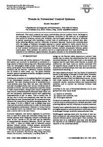
Let’s take Γ = 0.16, θ = 0.0281. Fig. 2 shows the fault estimation performance, from which we can see that fˆ(k) follows f (k) rapidly with a very small overshoot. 6. CONCLUSION In this paper, we discuss the fault estimation problem for NCSs with both linear and a kind of nonlinear plants.
1906
17th IFAC World Congress (IFAC'08) Seoul, Korea, July 6-11, 2008
The considered NCSs are modelled as T-S systems, which is suitable for adaptive observer-based fault estimation. Then, we use the Lyapunov function to prove that the proposed fault diagnosis method can make the estimation error converge to the given region. Simulation results of a motor system are given to verify the effectiveness of the proposed method. Further, the purpose of the designed fault estimation method is to achieve the active fault-tolerant control. Ref. Neˇsi´c et al. (1999) has provided a sufficient condition for stabilization of NCSs via discrete-time approximations, which is used to model the NCSs. So the FE method proposed in this paper can be employed to reconfigure the controller to recover the system performance, that is also our future work. 1.5 fault estimates fault
1
0.5
0
−0.5
−1
−1.5 0
1
2
3
4
5
6
7
8
9
10
sec
Fig. 2. Fault estimation ACKNOWLEDGEMENTS Peng Shi is grateful to the support from the starting research grant of Nanjing University of Aeronautics and Astronautics. REFERENCES D. Berdjag, C. Christophe, V. Cocquempot, and B. Jiang. Nonlinear model decomposition for robust fault detection and isolation using algebraic tools, Int. J. Innovative Computing, Information and Control, 6:1337–1354, 2006. M. Blanke, M. Kinnaert, J. Lunze, and M. Staroswiecki. Diagnosis and Fault-Tolerant Control. Springer Verlag, Berlin, Heidelberg, 2003. J. Chen, and R. J. Patton. Robust Model-based Fault Diagnosis for Dynamics Systems. Boston: Kluwer Academic Publishers, 1999. F. N. Chowdhury, B. Jiang, and C. M. Belcastro. Reduction of false alarms in fault detection problems, Int. J. Innovative Computing, Information and Control, 2: 481–490, 2006. J. J. Gertler. Fault Detection and Diagnosis in Engineering Systems . New York: Marcel Dekker, 1998. B. Jiang, J. L. Wang, and Y. C. Soh. An adaptive technique for robust diagnosis of faults with independent effects on system outputs, Int. J. of Control, 75:792–802, 2002.
C. Kambhampati, R. Patton and F. Uppal, Reconfiguration in networked control systems: fault tolerant control and plug and play, Proc. of the 6th IFAC Safeprocess, Beijing, 126–131, 2006. ¨ Ozg¨ ¨ uner, and H. Chan. Stability of linear R. Krtolica, U. feedback systems with random communication delays, Int. J. of Control, 59:925–953, 1994. Z. H. Mao, B. Jiang, and P. Shi. H∞ fault detection filter design for networked control systems modelled by discrete Markovian jump systems, IET Control Theory and Application, 1:1336–1343, 2007. D. Neˇsi´c, and A. R. Teel. Lp stability of networked control systems, Proc. of 42nd IEEE Conference on Decision and Control, Maui, Hawaii, USA, 1188–1193, 2003. D. Neˇsi´c, and A. R. Teel. Input-to-state stability of networked control systems, Automatica, 40:2121–2128, 2004. D. Neˇsi´c, A. R. Teel, and P. V. Kokotovi´c. Suffcient conditions for stabilization of sampled-data nonlinear systems via discrete-time approximations, Systems and Control letters, 38:259–270, 1999. S. K. Nguang, P. Shi, and S. Ding. Fault Detection for Uncertain Fuzzy Systems: An LMI Approach, IEEE Trans on Fuzzy Systems, in press, 2007. S. K. Nguang, P. Shi, and S. Ding. Delay dependent fault estimation for uncertain time delay nonlinear systems: an LMI approach, Int. J. Robust and Nonlinear Control, 32:371–379, 2006. D. Sauter and T. Boukhobza, Robustness against unknown networked induced delays of observer based FDI, Proc. of the 6th IFAC Safeprocess, Beijing, 300–305, 2006. E. I. Silva, G. C. Goodwin, D. E. Quevedo and S. Milan, Optimal noise shaping for networked control systems, Proc. of European Contorl Conference, Kos, Greece, 577–584, 2007. M. I. Spong, R. Peresada, S. M. Marino, and D. G. Taylor. Feedback linearizing control of switched reluctance motors, IEEE Trans. on Automatic Control, 32:371–379, 1987. G. C. Walsh, and H. Ye. Performance evaluation of control networks, IEEE Control Syst. Mag., 21:57–65, 2001. G. C. Walsh, H. Ye, and L. G. Bushnell. Stability analysis of networked control systems, IEEE Trans. Contr. Syst. Technol., 10:438–446, 2002. H. Ye, and S. X. Ding. Fault detection of networked control systems with networkinduced delay, Proc. of 8th International Conference on Control, Automation, Robotics and Vision, Kunming, China, 294-297, 2004. W. Zhang, M. S. Branicky, and S. M. Philips. Stability of networked control systems, IEEE Control System Magazine, 21:84–99, 2001. P. Zhang, and S. X. Ding. Fault detection of networked control systems with limited communication, Proc. of the 6th IFAC Safeprocess, Beijing, 1135–1140, 2006. Y. Zheng, H. J. Fang, and H. O. Wang. Takagi-Sugeno fuzzy-model-based fault detection for networked control systems with markov delays, IEEE Trans. on Systems, Man, and Cybernetics - Part B: Cybernetics, 36:924– 929, 2006. M. Zhong, H. Ye, P. Shi, and G. Wang. Fault detection for Markovian jump systems, IEE Control Theory Appl., 152:397–402, 2005.
1907