Hindawi Publishing Corporation e Scientific World Journal Volume 2014, Article ID 814245, 8 pages http://dx.doi.org/10.1155/2014/814245
Research Article Comprehensive Control of Networked Control Systems with Multistep Delay Jie Jiang1 and Changlin Ma2 1 2
College of Information System and Management, National University of Defense Technology, Changsha 410073, China School of Computer, Central China Normal University, Wuhan 430079, China
Correspondence should be addressed to Changlin Ma;
[email protected] Received 23 February 2014; Revised 16 May 2014; Accepted 5 June 2014; Published 1 July 2014 Academic Editor: Zhi Wang Copyright © 2014 J. Jiang and C. Ma. This is an open access article distributed under the Creative Commons Attribution License, which permits unrestricted use, distribution, and reproduction in any medium, provided the original work is properly cited. In networked control systems with multi-step delay, long time-delay causes vacant sampling and controller design difficulty. In order to solve the above problems, comprehensive control methods are proposed in this paper. Time-delay compensation control and linear-quadratic-Guassian (LQG) optimal control are adopted and the systems switch different controllers between two different states. LQG optimal controller is used with probability 1 − 𝛼 in normal state, which is shown to render the systems mean square exponentially stable. Time-delay compensation controller is used with probability 𝛼 in abnormal state to compensate vacant sampling and long time-delay. In addition, a buffer window is established at the actuator of the systems to store some history control inputs which are used to estimate the control state of present sampling period under the vacant sampling cases. The comprehensive control methods simplify control design which is easier to be implemented in engineering. The performance of the systems is also improved. Simulation results verify the validity of the proposed theory.
1. Introduction Feedback control systems in which control loops are closed through a real-time network are called networked control systems (NCSs) [1, 2]. This type of systems has many advantages such as flexible system design, simple installation and maintenance, increased system agility, and reduced system wiring. Compared with conventional point-to-point control systems, however, the insertion of communication network in the feedback control loop makes the analysis and design of NCSs more complex. Conventional control theory with many ideal assumptions, such as synchronized control and nondelayed sensing and actuation, has to be reevaluated before it is applied to NCSs. The existence of network in NCSs inevitably induces some nondeterministic phenomena, especially networkinduced delay, which will degrade the performance of control systems and even destabilize the systems. The networkinduced delay mainly comes from two resources: sensor-tocontroller delay and controller-to-actuator delay. It is of great
significance to explore suitable control methods under the stochastic delay in NCSs to improve the system performance. Some researchers studied stochastic time-delay and the optimal controllers of NCSs whose network-induced delay was shorter than a sampling period [3–5]. Nevertheless, the network-induced delay is longer than one sampling period in many cases. Substantial efforts have been done for the nonlinear NCSs with time-varying delay. A time-based neuron-dynamicprogramming (NDP) optimal control scheme for uncertain nonlinear NCSs was introduced by using output feedback and without utilizing value and policy iterations [6]. Closed-loop stability in the mean was demonstrated by selecting novel neural-network (NN) update laws. However, the stochastic characteristic of time-delay was not referred in the optimal control design. Cao [7] provided improved time-delaydependent stability criteria for multi-input and multi-output (MIMO) NCSs with nonlinear perturbations. Related control methods and simulations were not given to support the proposed theory. A high frequency NCS was described by
2 a time-varying delayed delta operator system with a high frequency constraint [8]. An improved stability condition was given for the delta operator system by using a generalized Kalman-Yakubovic-Popov lemma. They did not discuss the stochastic characteristic of time-delay and concrete control methods. In [9], optimizing controller design of real-time NCSs was presented based on different models. For timedelay less than one sampling interval, they modeled the system as a time-invariant control system with constant timedelay. For time-delay greater than one sampling interval, they modeled it as a jump linear control system. Nevertheless, NCSs models should be nonlinear because of time-varying delay. Using the Lyapunov-Krasovskii method, a sufficient condition for asymptotic stability of nonlinear NCSs was provided in [10]. Measured values were asynchronously sampled and transmitted over multiple communications links. The effects of communication in each link were captured by a time-varying delay element. In order to avoid complexities of these kinds of nonlinear NCSs, an assumption of delay bound was made under which the NCSs models were not sensitive to asynchrony of sampling and transmission between different links. With regard to the characteristic of uncertain delay in NCSs, some researchers proposed predictive control methods to compensate time-delay whose probability distribution was unknown [11–14]. The stochastic time-delay system was transformed to a deterministic delay system by placing a special amount of buffers at the nodes in NCSs. Multistep predicting controllers were designed to improve system performance through model matching and multistep predictive output compensation. However, this kind of models is too complex and has high computational cost due to the uncertainty of time-varying delay. When network-induced delay has a known probability distribution and is longer than one sampling period, Yu et al. [15] proposed a control mode: sensor and actuator were time-driven and controller was event-driven. Ma and Fang [16] put forward a time-division control mode: sensor was time-driven, controller was event-driven, and actuator was time-division-driven. Under the two kinds of control modes, perhaps there were not new control inputs arriving at the actuator during a sampling period because of data congestion or network bandwidth limitation. In this case the old control input of last sampling period continued acting on the plant, which might induce long time-delay. This kind of situation is called vacant sampling. The vacant sampling in NCSs may degrade the performance of control systems and even destabilize the systems. Furthermore, it will make optimal controller design difficult to be implemented in engineering when the time-delay of NCSs is too long. It is important to take some measures for compensating vacant sampling and long time-delay. To solve all the aforementioned problems, comprehensive control methods of NCSs are proposed in this paper. Timedelay compensation control and linear-quadratic-Guassian (LQG) optimal control are adopted and the systems switch different controllers between two different states. LQG optimal controller is used with probability 1 − 𝛼 in normal state,
The Scientific World Journal which is shown to render the systems mean square exponentially stable and guarantees the performance of NCSs with big probability. Combined with the strength of predictive control methods, time-delay compensation controller is used with probability 𝛼 in abnormal state with long delay and compensates vacant sampling and long time-delay. The stochastic characteristic of time-delay is also considered to design the optimal control of NCSs. The proposed comprehensive control methods reduce the complexities of system control and computational cost under the guarantee of improving system performance. The rest of this paper is organized as follows. Section 2 describes comprehensive control methods of NCSs. Simulations are given in Section 3, followed by conclusions in Section 4.
2. Description of Comprehensive Control Methods The stochastic delay in NCSs mainly comes from two resources: sensor-to-controller delay 𝜏sc and controller-toactuator delay 𝜏ca . Assume that network-induced delay 𝜏 has a known probability distribution function and 𝜏 = 𝜏sc + 𝜏ca ≤ 𝑝𝑇 (𝑝 is a positive integer, 𝑝 ≥ 2, and 𝑇 is the sampling period of sensor). Now, we describe the model of NCSs. We assume the state equation of plant is linear time-invariant which is expressed as ⋅
𝑥(𝑡)= 𝐴𝑥 (𝑡) + 𝐵𝑢 (𝑡) ,
𝑦 (𝑡) = 𝐶𝑥 (𝑡) ,
(1)
where 𝑥(𝑡) ∈ 𝑅𝑛 , 𝑢(𝑡) ∈ 𝑅𝑚 . 𝐴, 𝐵, and 𝐶 are matrices of appropriate sizes. Discretizing (1) separately under Yu’s control mode [15] and Ma’s control mode [16] over a sampling interval [𝑘𝑇, (𝑘 + 1)𝑇), we have a stochastic NCSs model as follows: 𝑝
𝑥𝑘+1 = 𝐴 𝑐 𝑥𝑘 + ∑𝐵𝑗𝑘 𝑢𝑘−𝑗 , 𝑗=0
𝑦𝑘 = 𝐶𝑥𝑘 ,
(2)
where under Yu’s control mode: 𝑥𝑘 = 𝑥 (𝑘𝑇) ,
𝑦𝑘 = 𝑦 (𝑘𝑇) ,
𝐴 𝑐 = 𝑒𝐴𝑇 ,
𝑇
𝐵𝑗𝑘 = 𝛽𝑗 Γ = 𝛽𝑗 ∫ 𝑒𝐴𝑡 𝑑𝑡 ⋅ 𝐵, 0
𝛽0 , . . . , 𝛽𝑝 ∈ {0, 1}
(𝑗 = 0, . . . , 𝑝) ,
and under Ma’s control mode: 𝑥𝑘 = 𝑥 (𝑘𝑇) ,
𝑦𝑘 = 𝑦 (𝑘𝑇) ,
𝐴 𝑐 = 𝑒𝐴𝑇 ,
(3)
The Scientific World Journal 𝐵𝑗𝑘 = ∫
𝑇/(𝑝+1)
0
3 { 0.5, { { 𝑏𝑗 = { { {1.5, {
𝑒𝐴(𝑇−𝑠) 𝑘 −𝐴𝑡𝑝+1
× (𝛼𝑝𝑗 𝑒
𝑘 −𝐴𝑡𝑖+1
+ ⋅ ⋅ ⋅ + 𝛼𝑖𝑗 𝑒 𝑘
+ ⋅ ⋅ ⋅ + 𝛼0𝑗 𝑒−𝐴𝑡1 ) 𝑑𝑠 ⋅ 𝐵,
𝛼𝑖0 , . . . , 𝛼𝑖𝑝 ∈ {0, 1} ,
𝑝
∑ 𝛼𝑖𝑗 = 1,
(𝑖 = 0, . . . , 𝑝, 𝑗 = 0, . . . , 𝑝) ,
𝑗=0
(4) 𝐵𝑗𝑘 (𝑗 = 0, . . . , 𝑝) are stochastic variables. Assume that the transfer delay from sensor to actuator at the moment 𝑘𝑇 is 𝑑𝑘 (0 ⩽ 𝑑𝑘 ⩽ 𝑝). We can conclude that {𝑑𝑘 , 𝑘 = 0, 1, 2, . . .} is a Markov chain. The state transition matrixes under Yu’s control mode and Ma’s control mode can be derived [15, 16]. Under the two kinds of control modes above, perhaps there is vacant sampling during a sampling period because of data congestion or network bandwidth limitation. For the sake of avoiding the vacant sampling in NCSs, time-delay compensation control is put forward and used to compensate long time-delay in this paper. It is described as follows. A buffer window is established at actuator to store some history control inputs {𝑢𝑘−𝑝 , 𝑢𝑘−𝑝+1 , . . . , 𝑢𝑘−1 }. There are at most 𝑝 history control inputs in the window. If vacant sampling occurs in NCSs over a sampling interval [𝑘𝑇, (𝑘 + 1)𝑇), the history control inputs are used to estimate the control state of present sampling period. According to the time order of history control inputs, some weights are derived. The average value of history control inputs with weights is calculated to act on plant instead of the old control input of last sampling period. In terms of the synthetic effects of these history control inputs, the performance of NCSs is improved. At the beginning, the initial values of control inputs in the buffer window are set as 0. We use the following equation to estimate control input which is denoted as 𝑢𝑘 over a sampling interval [𝑘𝑇, (𝑘 + 1)𝑇). The estimation value of 𝑢𝑘 is denoted by ∑𝑘−1 { 𝑖=1 𝑎𝑖 𝑢𝑖 { , { { { 𝑘−1 𝑢̂𝑘 = { 𝑘−1 { { ∑𝑗=𝑘−𝑝 𝑏𝑗 𝑢𝑗 { { , 𝑝 {
(𝑖 = 1, . . . , [ (𝑖 = [
(7)
where [(𝑘 − 1)/2] is the integer function of (𝑘 − 1)/2 and [𝑝/2] is the integer function of 𝑝/2. The time-delay compensation control guarantees not only the priority of history control inputs with smaller delay but also the synthetic effects of all history control inputs. In NCSs, optimal control is often used to improve system performance and stabilize the whole system. Now we design the LQG optimal controller of system (2). Theorem 1. With the system having full state information, the LQG optimal control law for NCSs system (2) is 𝑇
𝑇 𝑇 𝑇 , 𝑢𝑘−𝑝+1 , . . . , 𝑢𝑘−1 ] , 𝑢𝑘 = −𝐿 𝑘 [𝑥𝑘𝑇 , 𝑢𝑘−𝑝
(8)
where 𝐿 𝑘 = [𝐸 (𝐵𝑘𝑇 𝑆𝑘+1 𝐵𝑘 ) + 𝑅 ]
−1
⋅ 𝐸 (𝐵𝑘𝑇 𝑆𝑘+1 𝐴 𝑘 ) ,
𝑆𝑘 = 𝐸 (𝐴𝑇𝑘 𝑆𝑘+1 𝐴 𝑘 ) + 𝑄 − 𝐿𝑇𝑘 [𝐸 (𝐵𝑘𝑇 𝑆𝑘+1 𝐵𝑘 ) + 𝑅 ] 𝐿 𝑘 ,
(9)
and it renders system (2) mean square exponentially stable. Proof. In this paper, we design a control law of the stochastic open-loop NCSs as expressed in (2) to minimize the cost function 𝑁−1
𝑇 𝑃𝑁𝑥𝑁 + ∑ [𝑥𝑘𝑇 𝑄𝑥𝑘 + 𝑢𝑘𝑇 𝑅𝑢𝑘 ]} , 𝐽𝑁 = 𝐸 {𝑥𝑁
(10)
𝑘=0
where 𝑃𝑁 and 𝑄 are symmetric and positive semidefinite and 𝑅 is symmetric and positive definite. At first we introduce a new state variable 𝑇
𝑇 𝑇 𝑇 , 𝑢𝑘−𝑝+1 , . . . , 𝑢𝑘−1 ] ∈ 𝑅𝑛+𝑝𝑚 . 𝑧𝑘 = [𝑥𝑘𝑇 , 𝑢𝑘−𝑝
(11)
Then system (2) can be expressed as follows: 𝑧𝑘+1 = 𝐴 𝑘 𝑧𝑘 + 𝐵𝑘 𝑢𝑘 ,
(12)
where (𝑘 < 𝑝) , (5) (𝑘 ≥ 𝑝) ,
where {𝑎𝑖 , 𝑖 = 1, . . . , 𝑘 − 1}, {𝑏𝑗 , 𝑗 = 𝑘 − 𝑝, . . . , 𝑘 − 1} are weight sequences for history control inputs. They are calculated as follows: 0.5, { { { 𝑎𝑖 = { { { 1.5, {
𝑝 (𝑗 = 𝑘 − 𝑝, . . . , 𝑘 − [ ]) , 2 𝑝 (𝑗 = 𝑘 − [ ] + 1, . . . , 𝑘 − 1) , 2
𝑘−1 ]) , 2
𝑘−1 ] + 1, . . . , 𝑘 − 1) , 2
(6)
[ [ [ [ [ 𝐴𝑘 = [ [ [ [ [ [
𝑘 ⋅ ⋅ ⋅ 𝐵2𝑘 𝐵1𝑘 𝐴 𝑐 𝐵𝑝𝑘 𝐵𝑝−1
0 .. .
0 .. .
𝐼𝑚 .. .
0
0
0
[0
0
0 𝐵0𝑘
] ] 0] ] ] d 0 0] ], ] ] ⋅ ⋅ ⋅ 0 𝐼𝑚 ] ]
⋅⋅⋅ 0
⋅⋅⋅ 0
[ ] [0] [ ] .] 𝐵𝑘 = [ [ .. ] . [ ] [0] [𝐼𝑚 ]
0]
(13)
4
The Scientific World Journal 𝑁−1
Cost function (10) is equivalent to
+ ∑ [𝑧𝑙𝑇 𝑄 𝑧𝑙 + 𝑢𝑙𝑇 𝑅 𝑢𝑙 ]
𝑁−1
𝑇 𝐽𝑁 = 𝐸 {𝑧𝑁 𝑃𝑁𝑧𝑁 + ∑ [𝑧𝑘𝑇 𝑄 𝑧𝑘 + 𝑢𝑘𝑇 𝑅 𝑢𝑘 ]} ,
𝑙=𝑘+1
(14)
𝑘=0
| 𝑧𝑘+1 } | 𝑧𝑘 }
where [ [ [ [ [ [ 𝑃𝑁 =[ [ [ [ [ [ [ [
0 1 0 ( )𝑅 (𝑝 + 1)
𝑃𝑁
0
0
.. .
.. .
0
0
0
⋅⋅⋅
0
⋅⋅⋅
2 )𝑅 ⋅⋅⋅ ( (𝑝 + 1) .. . d 0
⋅⋅⋅
𝑄 0 0 [ 1 [0 ( )𝑅 0 [ (𝑝 + 1) [ [ 1 [0 )𝑅 0 ( 𝑄 = [ [ (𝑝 + 1) [. .. .. [. [. . . [ [ 0 0 0 [ 𝑅 = (
⋅⋅⋅ ⋅⋅⋅ ⋅⋅⋅ d ⋅⋅⋅
0
] ] 0 ] ] ] ] 0 ], ] ] ] ] 0 ] ] 𝑝 )𝑅 ( (𝑝 + 1) ] ] ] 0 ] ] ] ] 0 ], ] ] ] ] 0 ] ] 1 )𝑅 ( (𝑝 + 1) ]
1 ) 𝑅. (𝑝 + 1)
and 𝑄 are symmetric and positive semidefinite and Now 𝑅 is symmetric and positive definite. Minimizing cost function (14) is equivalent to minimizing cost function (10). At first we write out Bellman functional equation of cost function (14). Consider min𝐽𝑘 = 𝑢 min ,...,𝑢 𝑘
𝑁−1
= 𝐸 {𝑢 min ,...,𝑢 𝑘
𝑁−1
𝑁−1
+ ∑
𝑇 {𝑧𝑁 𝑃𝑁𝑧𝑁
𝑙=𝑘
[𝑧𝑙𝑇 𝑄 𝑧𝑙
𝑁−1
+ ∑ 𝑙=𝑘
+
[𝑧𝑙𝑇 𝑄 𝑧𝑙
𝑢𝑙𝑇 𝑅 𝑢𝑙 ]} +
𝑢𝑙𝑇 𝑅 𝑢𝑙 ]}}
𝑇 = 𝐸 {𝑢 min 𝐸 {𝑧𝑁 𝑃𝑁𝑧𝑁 ,...,𝑢 𝑘
𝑁−1
𝑁−1
+ ∑ [𝑧𝑙𝑇 𝑄 𝑧𝑙 + 𝑢𝑙𝑇𝑅 𝑢𝑙 ] | 𝑧𝑘 } 𝑙=𝑘
= 𝐸 [𝑉 (𝑧𝑘 , 𝑘)] ,
{𝑧𝑘𝑇 𝑄 𝑧𝑘 +𝑢𝑘𝑇𝑅 𝑢𝑘 +𝐸 {𝑉 (𝑧𝑘+1 , 𝑘+1) | 𝑧𝑘 }} . = min 𝑢 𝑘
(16) Equation (16) is Bellman functional equation. Then, we prove that the solution of (16) is as follows: 𝑉 (𝑧𝑘 , 𝑘) = 𝑧𝑘𝑇 𝑆𝑘 𝑧𝑘 + 𝑠𝑘 ,
where 𝑆𝑘 and 𝑠𝑘 are nondeterministic. We prove (17) with mathematical induction. Let 𝑞 express time. When 𝑞 = 𝑁, the conclusion is apparently correct. If we suppose that when 𝑞 = 𝑘 + 1 the conclusion is correct, we will prove that when 𝑞 = 𝑘 the conclusion is also correct. Consider
𝑇 𝑇 𝐸 {𝑧𝑁 𝑃𝑁𝑧𝑁 | 𝑧𝑁} = 𝑧𝑁 𝑃𝑁𝑧𝑁. 𝑉 (𝑧𝑁, 𝑁) = min 𝑢
(18)
𝑁
Let 𝑆𝑁 = 𝑃𝑁 and 𝑠𝑁 = 0 and then (17) holds.
(b) When 𝑞 = 𝑘 + 1, (17) holds. Now, we have 𝑇 𝑉 (𝑧𝑘+1 , 𝑘 + 1) = 𝑧𝑘+1 𝑆𝑘+1 𝑧𝑘+1 + 𝑠𝑘+1 ,
(19)
𝑇 𝐸 {𝑉 (𝑧𝑘+1 , 𝑘 + 1) | 𝑧𝑘 } = 𝐸 {𝑧𝑘+1 𝑆𝑘+1 𝑧𝑘+1 | 𝑧𝑘 } + 𝑠𝑘+1 .
Using (12) we can conclude 𝐸 {𝑉 (𝑧𝑘+1 , 𝑘 + 1) | 𝑧𝑘 } 𝑇
= 𝐸 {(𝐴 𝑘 𝑧𝑘 + 𝐵𝑘 𝑢𝑘 ) ⋅ 𝑆𝑘+1 ⋅ (𝐴 𝑘 𝑧𝑘 + 𝐵𝑘 𝑢𝑘 ) | 𝑧𝑘 } + 𝑠𝑘+1
𝑉 (𝑧𝑘 , 𝑘)
(17)
(a) 𝑞 = 𝑁
𝑇 𝐸 {𝑧𝑁 𝑃𝑁𝑧𝑁
𝑘
0
(15) 𝑃𝑁
= min 𝐸 {𝑧𝑘𝑇 𝑄 𝑧𝑘 +𝑢𝑘𝑇𝑅 𝑢𝑘 +𝑉 (𝑧𝑘+1 , 𝑘 + 1) | 𝑧𝑘 } 𝑢
(20)
𝑇
= min 𝐸 {𝑧𝑘𝑇 𝑄 𝑧𝑘 + 𝑢𝑘𝑇 𝑅 𝑢𝑘 𝑢 𝑘
𝑇 + 𝑢 min 𝐸 {𝑧𝑁 𝑃𝑁𝑧𝑁 ...,𝑢 𝑘+1
𝑁−1
= (𝐴 𝑘 𝑧𝑘 + 𝐵𝑘 𝑢𝑘 ) ⋅ 𝑆𝑘+1 ⋅ (𝐴 𝑘 𝑧𝑘 + 𝐵𝑘 𝑢𝑘 ) + tr 𝑆𝑘+1 𝑅1 + 𝑠𝑘+1 ,
where 𝑅1 = 𝐸{(𝑧𝑘+1 − 𝐸{𝑧𝑘+1 })(𝑧𝑘+1 − 𝐸{𝑧𝑘+1 })𝑇 }.
The Scientific World Journal
5
(c) 𝑞 = 𝑘 Using (20) and considering (16), we can derive
Definition 2 (see [18]). Assume that the distribution function of population 𝑋 is 𝐹(𝑥; 𝜃), 𝜃 is an unknown parameter, and 𝜃 ∈ Θ. For a constant 𝛼 (0 < 𝛼 < 1), if statistic variable 𝜃 = 𝜃(𝑋1 , 𝑋2 , . . . , 𝑋𝑛 ), which is derived from the samples 𝑋1 , 𝑋2 , . . . , 𝑋𝑛 , meets the following equation:
𝑉 (𝑧𝑘 , 𝑘) 𝐸 {𝑧𝑘𝑇 𝑄 𝑧𝑘 + 𝑢𝑘𝑇 𝑅 𝑢𝑘 = min 𝑢 𝑘
𝑃 {𝜃 < 𝜃 (𝑋1 , 𝑋2 , . . . , 𝑋𝑛 )} = 1 − 𝛼,
𝑇
+ 𝐸 {(𝐴 𝑘 𝑧𝑘 + 𝐵𝑘 𝑢𝑘 ) ⋅ 𝑆𝑘+1 ⋅ (𝐴 𝑘 𝑧𝑘 + 𝐵𝑘 𝑢𝑘 ) | 𝑧𝑘 } + 𝑠𝑘+1 } {𝑧𝑘𝑇 𝑆𝑘 𝑧𝑘 + [𝑢𝑘 + 𝐿 𝑘 𝑧𝑘 ] = min 𝑢
(21)
𝑇
𝑘
⋅ [𝐸 (𝐵𝑘𝑇 𝑆𝑘+1 𝐵𝑘 ) + 𝑅 ] ⋅ [𝑢𝑘 + 𝐿 𝑘 𝑧𝑘 ] + tr 𝑆𝑘+1 𝑅1 + 𝑠𝑘+1 } , where 𝐿 𝑘 = [𝐸 (𝐵𝑘𝑇 𝑆𝑘+1 𝐵𝑘 ) + 𝑅 ]
−1
⋅ 𝐸 (𝐵𝑘𝑇 𝑆𝑘+1 𝐴 𝑘 ) ,
𝑆𝑘 = 𝐸 (𝐴𝑇𝑘 𝑆𝑘+1 𝐴 𝑘 ) + 𝑄 − 𝐿𝑇𝑘 [𝐸 (𝐵𝑘𝑇 𝑆𝑘+1 𝐵𝑘 ) + 𝑅 ] 𝐿 𝑘 , 𝑠𝑘 = tr 𝑆𝑘+1 𝑅1 + 𝑠𝑘+1 . (22) Letting 𝑢𝑘 = −𝐿 𝑘 𝑧𝑘 , 𝑉(𝑧𝑘 , 𝑘) is the minimum cost. Consider 𝑉 (𝑧𝑘 , 𝑘) = 𝑧𝑘𝑇 𝑆𝑘 𝑧𝑘 + 𝑠𝑘 .
(23)
Thus, when 𝑞 = 𝑘, (17) also holds, and when 𝑢𝑘 = −𝐿 𝑘 𝑧𝑘 𝑇
𝑇 𝑇 𝑇 = −𝐿 𝑘 [𝑥𝑘𝑇 , 𝑢𝑘−𝑝 , 𝑢𝑘−𝑝+1 , . . . , 𝑢𝑘−1 ] ,
(24)
𝑉(𝑧𝑘 , 𝑘) is minimum cost, so is 𝐽𝑘 . Similar to the proving process in [17], we can conclude that LQG optimal control law (8) renders system (2) mean square exponentially stable. Now we prove Theorem 1. In practical application of NCSs, network-induced delay is often longer than one sampling period. When the timedelay of NCSs is too long, it will make optimal controller design difficult to be implemented in engineering. In order to reduce the complexities and computational cost of system control, comprehensive control methods are proposed whose main idea is as follows. When time-delay is smaller than a suitable delay bound, optimal controller (8) is used to stabilize the systems during most of running time, which can make optimal control easier to be implemented. While time-delay is bigger than the delay bound, time-delay compensation controller (5) is used to compensate vacant sampling and long time-delay. The comprehensive control methods are based on 𝛼 confidence level in this paper. Normal and abnormal states are defined for the delay’s two different cases. The related definitions are given as follows.
(25)
then stochastic interval (−∞ 𝜃) is called single-side confidence interval with confidence level 1 − 𝛼. 𝜃 that is called single-side confidence upper limit. Now we discuss the single-side confidence interval of time-delay 𝜏 based on confidence level 𝛼 in NCSs. For given constant 𝛼 (0 < 𝛼 < 1), the single-side confidence upper limit 𝜏 = 𝑝 𝑇 (𝑝 is a positive integer and 𝑝 < 𝑝) of 𝜏 can be derived. On the basis of 𝜏 and 𝜏, normal and abnormal states are defined as follows. Definition 3. When 𝜏 < 𝜏 and 𝑃{𝜏 < 𝜏} = 1 − 𝛼, the system state is called normal state. When 𝜏 ≤ 𝜏 ≤ 𝑝𝑇 and 𝑃{𝜏 ≤ 𝜏 ≤ 𝑝𝑇} = 𝛼, the system state is called abnormal state. In NCSs, time-delay 𝜏 does not always access or reach the maximum delay 𝑝𝑇. In general cases, it is near expectation value 𝐸{𝜏} with big probability. We can choose suitable confidence level 𝛼 to make random event {𝜏 < 𝜏} be a bigprobability event when random event {𝜏 ≤ 𝜏 ≤ 𝑝𝑇} is a small-probability event. The probability of the systems in normal state is 1 − 𝛼. LQG optimal controller (8) is adopted in normal state, which is shown to render the systems mean square exponentially stable during most of running time. The probability of the systems in abnormal state is 𝛼. Time-delay compensation controller (5) is adopted in abnormal state to compensate vacant sampling and long time-delay. Using Schur complement and Cone-complement linear technique, an approximate solution of control law was obtained in [19], which rendered system (2) asymptotically stable. It is described as follows. Theorem 4. If there exist 𝑃 > 0, 𝑀 > 0, 𝑄 > 0, and 𝑁 > 0, 𝐺, 𝑋, 𝑌, Ζ, such that ℓ11 −𝑌 𝐴𝑇𝑘
[ [ 𝑇 [−𝑌 −𝑄 𝐵𝑘𝑇 [ [ [ [ 𝐴 𝑘 𝐵𝑘 −𝑀 [ [ ℓ41
ℓ42
0
𝑇 ℓ41 𝑇 ℓ42
0
] ] ] ] ] < 0, ] ] ]
− (𝑝 − 1) 𝑁]
𝑋 𝑌 [ 𝑇 ] ≥ 0, 𝑌 Ζ 𝑃 𝐼𝑝𝑛 [ ] ≥ 0, 𝐼𝑝𝑛 𝑀 Ζ 𝐼𝑝𝑛 [ ] ≥ 0, 𝐼𝑝𝑛 𝑁
(26)
6
The Scientific World Journal
where
where 𝑥𝑘0
ℓ11 = −𝑃 + (𝑝 − 1) 𝑋 + 𝑌 + 𝑌𝑇 + 𝑄, ℓ41 = (𝑝 − 1) (𝐴 𝑘 − 𝐼𝑝𝑛 ) ,
(27)
ℓ42 = (𝑝 − 1) 𝐵𝑘 ,
𝐴𝑗 = [
then system (2) is asymptotically stable for any networkinduced delay 𝜏 satisfying 0 ≤ 𝜏 ≤ 𝑝𝑇 (𝑝 ≥ 2 is a positive integer).
When the maximum delay 𝑝𝑇 is known, the controller 𝑢𝑘 = 𝐺𝑥𝑘
(28)
can be obtained based on Theorem 4 using the MATLAB LMI Toolbox. Now we make some changes in the comprehensive control methods. LQG optimal controller (8) is adopted in normal state, which is shown to render the systems mean square exponentially stable. Controller (28) is adopted in abnormal state to compensate vacant sampling and long time-delay, which is shown to approximately render the systems asymptotically stable. Then the system model is described as follows. We denote the state variable and output of NCSs in 𝑓 𝑓 normal state and abnormal state as 𝑥𝑘0 , 𝑦𝑘0 , 𝑥𝑘 , and 𝑦𝑘 . Then the optimal controller in Theorem 1 can be written as
𝑢𝑘 = −𝐿 𝑘 𝑧𝑘 = − [𝐿0𝑘 𝐿𝑝𝑘 𝐿𝑝𝑘 −1 ⋅ ⋅ ⋅ 𝐿1𝑘 ] 𝑥𝑘0 [ 𝑢 ] [ 𝑘−𝑝 ] [ ] 𝑢 ] ⋅[ [ 𝑘−𝑝 +1 ] , [ .. ] [ . ] [ 𝑢𝑘−1 ] 1×𝑛
𝐿𝑖𝑘
(29)
1×𝑚
𝑓
𝑢𝑘 = 𝐺𝑥𝑘 .
(30)
From the discussion above, we get the comprehensive control model of system (2) 𝑥𝑘+1 = 𝐴0 𝑥𝑘 + ∑𝐴𝑗 𝑥𝑘−𝑗
0 0 ], 0 𝐼𝑛
𝐶=[ 𝐷𝑗 = [
𝐶 0 ], 0 𝐶
𝐷𝑗𝑘 0 ], 0 0
(32)
{ 𝑗−𝑖 { { (1 ≤ 𝑗 ≤ 𝑝 ) , − ∑ 𝐵𝑖𝑘 𝐿 𝑘 , { { { 𝑖=0 𝐷𝑗𝑘 = { 𝑝 { { 𝑘 𝑗−𝑖 { { { − ∑ 𝐵𝑖 𝐿 𝑘 , (𝑝 + 1 ≤ 𝑗 ≤ 2𝑝 ) . { 𝑖=𝑗−𝑝
3. Simulations The simplified model of the inverted pendulum process is as follows [20]: ⋅ 0 1 0 𝑥(𝑡)= [ ] 𝑥 (𝑡) + [ ] 𝑢 (𝑡) , 1 0 1
2𝑝
+ ∑ 𝐵𝑗 𝑥𝑘−𝑗 + ∑ 𝐷𝑗 𝑢𝑘−𝑗 , 𝑗=1
(33)
𝑦 (𝑡) = [1 0] 𝑥 (𝑡) . In this paper, we use MatLab and C++ to simulate the comprehensive control methods on the networked inverted pendulum system that we construct based on NS2 [21]. In the simulations, parameters are selected as follows: 𝑇 = 0.05 s, 𝑃𝑁 = 𝑄 = [ 10 01 ], and 𝑅 = 0.1. It is assumed that the maximum network-induced delay is 3𝑇; that is, 𝑝 = 3. Using stochastic sampling experiment, we can get 𝜏 = 2𝑇 (𝑝 = 2) under confidence level parameter 𝛼 = 0.05. The state transition matrix under Yu’s control mode is 0.8 0.2 0 𝑄𝑀 = [0.4 0.1 0.5] . [0.4 0.1 0.5]
(34)
The state transition matrixes under Ma’s control mode are 1 0 0 𝑃𝑀1 = [0.88 0.12 0 ] , [0.82 0.08 0.1] 1 0 0 = [0.8889 0.1111 0 ] . 0.1 0.1] [ 0.8
(35)
Then by Theorem 1 we can get the optimal control input
𝑗=1
𝑦𝑘+1 = 𝐶𝑥𝑘+1 ,
𝐵𝑗 = [
𝑃𝑀2
𝑝
𝑗=𝑝 +1
0 𝐴 𝑐 − 𝐿0𝑘 𝐵0𝑘 ], 0 𝐴 𝑐 + 𝐺𝐵0𝑘
−𝐿0𝑘 𝐵𝑗𝑘 0 ], 0 𝐺𝐵𝑗𝑘
∈ 𝑅 and ∈𝑅 (𝑖 = 1, . . . , 𝑝 ). Time-delay where compensating controller (28) can be written as
𝑝
𝐴0 = [
𝑗−1
Proof. See proof of Theorem 1 in [19].
𝐿0𝑘
𝑥𝑘 = [ ] , 𝑓 [𝑥𝑘 ]
(31)
𝑢𝑘 = − [3.9760 3.9679] 𝑥𝑘 − 0.0085𝑢𝑘−2 − 0.0206𝑢𝑘−1 . (36) At first we use controller (5) as time-delay compensation controller. With the initial state value 𝑥(0) = [1 − 0.5]𝑇
The Scientific World Journal
7
1
1
0.8 0.5 0.6 0.4
0
0.2
−0.5
0
−1
−0.2
−0.4
−1.5
−0.6 −0.8
0
1
2
3
4
5
6
7
8
9
10
−2
0
1
2
3
Time (s) Method 1 x 1 Method 1 x 2 Method 2 x 1
Method 2 x 2 Method 3 x 1 Method 3 x 2
Method 1 x 1 Method 1 x 2 Method 2 x 1
4
5 6 Time (s)
7
8
9
10
Method 2 x 2 Method 3 x 1 Method 3 x 2
Figure 1: Curves of state response.
Figure 2: Curves of state response.
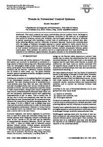
of the system, the simulation results of method 1 (method without considering comprehensive control methods under Ma’s control mode), method 2 (comprehensive control methods under Yu’s control mode), and method 3 (comprehensive control methods under Ma’s control mode) are given in Figure 1. Then we use controller (28) as time-delay compensation controller. By Theorem 4, we can obtain the control input 𝑢𝑘 = −[4.0571 4.0553]𝑥𝑘 . With the initial state value 𝑥(0) = [1 − 0.5]𝑇 of the system, the simulation results of method 1 (method without considering comprehensive control methods under Yu’s control mode), method 2 (comprehensive control methods under Yu’s control mode), and method 3 (comprehensive control methods under Ma’s control mode) are given in Figure 2. From Figures 1 and 2, we can see that the system performance is obviously improved under the comprehensive control methods which make NCSs faster to reach stability status. The simulation results show the validity of the proposed theory.
control effects than single control method. We will synthesize more optimal control methods in future work to further improve the performance of NCSs.
4. Conclusions In order to improve the performance of NCSs with multistep delay, comprehensive control methods based on confidence level are presented in this paper. Time-delay compensation control and LQG optimal control are adopted and the systems switch different controllers between two different states. LQG optimal control is used with probability 1 − 𝛼 in normal state, which is shown to render the systems mean square exponentially stable. Timedelay compensation control is used with probability 𝛼 in abnormal state. The comprehensive control methods simplify controller design and reduce computational cost. It is proved by simulations that the new control methods have better
Conflict of Interests The authors declare that there is no conflict of interests regarding the publication of this paper.
Acknowledgment This work is supported by NSFC under Grant no. 61202470.
References [1] W. Zhang, M. S. Branicky, and S. M. Phillips, “Stability of networked control systems,” IEEE Control Systems Magazine, vol. 21, no. 1, pp. 84–97, 2001. [2] J. Nilsson, Real-Time Control Systems with Delays, Department of Automatic Control, Lund Institute of Technology, Lund, Sweden, 1998. [3] Y. Q. Yang, D. Xu, and M. Tan, “Hybrid and stochastic stabilization analysis and H∞ control for networked control systems,” in Proceedings of the IEEE Conference on Robotics, Automation and Mechatronics, pp. 502–506, Singapore, December 2004. [4] F. Lian, J. Moyne, and D. Tilbury, “Network design consideration for distributed control systems,” IEEE Transactions on Control Systems Technology, vol. 10, no. 2, pp. 297–307, 2002. [5] R. Luck and A. Ray, “An observer-based compensator for distributed delays,” Automatica, vol. 26, no. 5, pp. 903–908, 1990. [6] X. Hao and S. Jagannathan, “Stochastic optimal controller design for uncertain nonlinear networked control system via neuro dynamic programming,” IEEE Transactions on Neural Networks and Learning Systems, vol. 24, no. 3, pp. 471–484, 2013.
8 [7] J. W. Cao, “Improved delay-dependent stability conditions for MIMO networked control systems with nonlinear perturbations,” The Scientific World Journal, vol. 2014, Article ID 196927, 4 pages, 2014. [8] H. J. Yang, Y. Q. Xia, P. Shi, and M. Y. Fu, “Stability analysis for high frequency networked control systems,” IEEE Transactions on Automatic Control, vol. 57, no. 10, pp. 2694–2700, 2012. [9] P. Wen, J. Cao, and Y. Li, “Design of high-performance networked real-time control systems,” IET Control Theory & Applications, vol. 1, no. 5, pp. 1329–1335, 2007. [10] B. Tavassoli, “Stability of nonlinear networked control systems over multiple communication links with asynchronous sampling,” IEEE Transactions on Automatic Control, vol. 59, no. 2, pp. 511–515, 2014. [11] Q. Zhu, H. Liu, and S. Hu, “The multi-step predicting controllers for deterministic networked control systems,” Binggong Xuebao/Acta Armamentarii, vol. 30, no. 8, pp. 1124–1128, 2009. [12] H. Jiwei, T. Liang, S. Hexu, and L. Zhaoming, “State predication controller design for a class of discrete networked control systems,” in Proceedings of the ISECS International Colloquium on Computing, Communication, Control, and Management (CCCM '08), pp. 193–197, Guangzhou, China, August 2008. [13] J. G. Wu and M. R. Fei, “Application of predictive functional control in deterministic networked control systems,” Journal of East China University of Science and Technology, vol. 32, no. 7, pp. 876–888, 2006. [14] J. G. Wu and M. R. Fei, “The networked control systems based on predictive functional control,” in Proceedings of the International Conference on Intelligent Computing (ICIC '06), vol. 4114, pp. 1085–1092, Kunming, China, 2006. [15] Z. Yu, H. Chen, and Y. Wang, “Research on control of network system with Markov delay characteristic,” in Proceedings of the 3th World Congress on Intelligent Control and Automation, pp. 3636–3640, Hefei, China, July 2000. [16] C. Ma and H. Fang, “Research on stochastic control of networked control systems,” Communications in Nonlinear Science and Numerical Simulation, vol. 14, no. 2, pp. 500–507, 2009. [17] S. S. Hu and Q. X. Zhu, “Stochastic optimal control and analysis of stability of networked control systems with long delay,” Automatica, vol. 39, no. 11, pp. 1877–1884, 2003. [18] Z. Cheng, S. Q. Xie, and C. Y. Pan, Probability Theory and Mathematical Statistics, Higher Education Press, Beijing, China, 2002. [19] C. L. Ma and H. J. Fang, “Stochastic stabilization analysis of networked control systems,” Journal of Systems Engineering and Electronics, vol. 18, no. 1, pp. 137–141, 2007. [20] P. Marti, R. Villa, J. M. Fuertes, and G. Fohler, “On real time control tasks schedulability,” in Proceedings of the European Control Conference, pp. 2227–2232, Porto, Portugal, 2001. [21] A. B. Soglo and X. Yang, “Networked control system simulation design and its application,” Tsinghua Science and Technology, vol. 11, no. 3, pp. 287–294, 2006.
The Scientific World Journal