ionosphere by assimilating both ground- and LEO-based GNSS observations into this ...... Penn State University, Pennsylvania, USA, in 1983. He has been with ...
IEEE TRANSACTIONS ON GEOSCIENCE AND REMOTE SENSING, VOL. 52, NO. 7, JULY 2014
3759
Observing System Simulation Experiment Study on Imaging the Ionosphere by Assimilating Observations From Ground GNSS, LEO-Based Radio Occultation and Ocean Reflection, and Cross Link Xinan Yue, William S. Schreiner, Ying-Hwa Kuo, John J. Braun, Yu-Cheng Lin, and Weixing Wan
Abstract—In this paper, a global ionospheric data assimilation model is constructed based on the empirical internationalreference-ionosphere model and the Kalman filter. A sparse matrix method is used to militate the huge computation and storage problems. A series of observing system simulation experiments has been performed based on the existing global ground-based global navigation satellite system (GNSS) network, the planned Constellation Observing System for Meteorology, Ionosphere, and Climate #2/Formosa Satellite Mission #7 (COSMIC-2/FORMOSAT-7) orbits, and the real global position system and GLObal NAvigation Satellite System (GLONASS) orbits. Specifically, the COSMIC-2 will have six 24◦ inclination satellites in 500-km altitude and six 72◦ inclination satellites in 800-km altitude. The slant total electron content of ground-based GNSS, radio occultation and ocean reflection (OR) of 12 low-Earthorbit satellites, and cross-link between COSMIC-2 low and high inclination satellites are simulated by the NeQuick model. The ORs show great impacts in specifying the ionosphere except over the inland area. It complements the existing ground-based GNSS network, which mainly observes the ionosphere over the land area. The 24◦ and 72◦ satellites can complement each other to optimize the global ionospheric specification. The COSMIC-2 mission is expected to contribute significantly to the accurate ionospheric nowcast. Its potential ability in ionospheric short-term forecast is also discussed. Index Terms—Constellation Observing System for Meteorology, Ionosphere, and Climate (COSMIC), data assimilation, electron density, global navigation satellite system (GNSS), ionosphere, ocean reflection, radio occultation.
I. I NTRODUCTION
T
HE ultraviolet radiation from the sun interacts with the upper atmosphere to form an ionized layer making up the
Manuscript received December 11, 2012; revised April 22, 2013 and July 22, 2013; accepted July 24, 2013. This material is based upon work supported by the National Science Foundation under Cooperative Agreement AGS-1033112. The work of W. Wan was supported by the National Science Foundation of China under Grants 41131066 and 40904037. X. Yue, W. S. Schreiner, Y.-H. Kuo, J. J. Braun, and Y.-C. Lin are with the Constellation Observing System for Meteorology, Ionosphere, and Climate Program Office, University Corporation for Atmospheric Research, Boulder, CO 80301 USA. W. Wan is with the Institute of Geology and Geophysics, Chinese Academy of Sciences, Beijing 100029, China. Color versions of one or more of the figures in this paper are available online at http://ieeexplore.ieee.org. Digital Object Identifier 10.1109/TGRS.2013.2275753
ionosphere through photoionization process. The ionosphere can influence the radio wave propagation in terms of reflection, refraction, absorption, and scattering. The accurate specification of the ionosphere, particularly the electron density, can benefit both the scientific research and technical applications such as the global navigation satellite system (GNSS), the large number of low Earth orbit (LEO) satellites that are flying in ionospheric altitude, and ground radar systems. Electron distribution in the ionosphere is caused by a number of processes, including ionization by solar extreme ultraviolet (EUV) radiation and particle precipitation, chemical reactions including charge exchange and reactions with the neutral gas, transport by neutral winds and ion drifts, and ambipolar diffusion. The ionosphere becomes disturbed as it reacts to certain types of activity such as solar flare, geomagnetic storm, and planetary wave and tide from the lower atmosphere. Because of the importance of imaging the ionospheric electron density, many computerized ionospheric tomography (CIT) techniques have been developed since the pioneering work of Austen et al. [2] and Fremouw et al. [7]. The most frequently used CIT techniques are the algebraic reconstruction technique (ART) and the multiplicative ART [1], [22]. Early imaging work was mainly undertaken using LEO satellite beacon total electron content (TEC) measurements that provided 2-D regional studies [21]. With the availability of LEO-based GNSS observations, 3-D ionospheric electron density imaging using both ground-based and LEO-based slant TEC data was proposed [10], [11]. The readers are recommended to see the review paper [5] for the detailed history of ionospheric imaging. There is a growing interest in ionospheric/thermospheric data assimilation studies because of the following reasons: 1) Increased requirements on accurate ionospheric nowcast and forecast by the space weather community given increased human activities in the near Earth space; 2) mature empirical models such as international reference ionosphere (IRI) and theoretical ionospheric models [e.g., National Center for Atmospheric Research Thermosphere-Ionosphere-Electrodynamics General Circulation Model (NCAR-TIEGCM)] are publicly available [5], [23]; 3) data assimilation methods such as the 3/4-D Var and Kalman filter are mature and have achieved big successes in meteorology and oceanography [4]; 4) more ionospheric
0196-2892 © 2013 IEEE. Personal use is permitted, but republication/redistribution requires IEEE permission. See http://www.ieee.org/publications_standards/publications/rights/index.html for more information.
3760
IEEE TRANSACTIONS ON GEOSCIENCE AND REMOTE SENSING, VOL. 52, NO. 7, JULY 2014
observations with good global coverage are available. These observations include the global ionosonde network, global GNSS network, multi-LEO-satellite in situ measurements, and LEObased GNSS radio occultation (RO) technique. Several data assimilation models have been developed in the past decade by the research community. The Utah State University developed a Global Assimilation of Ionospheric Measurements model based on a theoretical model and a Kalman filter [29]. A team from the University of Southern California and the Jet Propulsion Laboratory constructed a Global Assimilative Ionospheric Model using a different first-principle ionospheric model as the background model and 4-D variational and Kalman filter optimization methods [31]. Bust and Mitchell [5] built the Ionospheric Data Assimilation Three-Dimensional model using a 3-D variational data assimilation technique, which allowed ionospheric electron density to be imaged with respect to both space and time (4-D), by assimilating multisource observations into the background model. When retrieving the electron density profiles from RO measurements, the frequently used Abel inversion has significant error, particularly in low latitude and low altitude due to the spherical symmetry assumption [34], [38]. To improve the Abel inversion, we recently developed a data assimilation model to simultaneously assimilate multiple RO events into the model to try to provide the ionospheric horizontal information by the observation themselves [35], [36]. A series of simulation studies shows that the global data assimilation can improve the Abel inversion and offers an optimal RO electron density profile retrieval if sufficient ROs are available simultaneously. In addition, we extended the lower atmosphere reanalysis to the ionosphere by assimilating both ground- and LEO-based GNSS observations into this model [37]. The preliminary reanalysis during 2002–2011 shows significant improvement over the IRI predictions. Since the success of the Global Positioning System (GPS)/Meteorology experiment aboard the MicroLab 1 satellite in 1994, LEO-based RO has become an important and robust ionospheric sounding technique. After that, many satellite missions were successfully launched with RO payloads, accumulating a large number of RO data [20]. The most significant and recent contributor to the RO data set is the well-known Formosa Satellite Mission 3/Constellation Observing System for Meteorology, Ionosphere, and Climate (FORMOSAT-3/COSMIC, hereafter called COSMIC for short) [8], [24]. In comparison with other observations, GNSS RO has advantages of limb sounding geometry, higher vertical resolution, and fully global coverage from the perspective of data assimilation. RO observations have been proven to be an important data assimilation source for accurate ionospheric specification [12]. Due to the success of COSMIC/FORMOSAT-3, the Joint U.S.–Taiwan Executive Steering Committee has decided to move forward with a follow-on RO mission (COSMIC-2/FORMOSAT-7, named COSMIC-2 for short in this paper), which implies that the number of RO observations will increase rapidly in the near future [28], [36]. In addition, some LEO constellations based on new observation techniques, such as LEO-based GNSS ocean reflections (ORs) and LEO-to-LEO cross-links (CLs), are proposed. For example, The National Aeronautics and Space
Administration (NASA) recently sponsored a project called the Cyclone Global Navigation Satellite System (CYGNSS) with the aim of improving hurricane forecasting by better understanding the interactions between the sea and the air near the core of a storm (http://aoss-research.engin.umich.edu/missions/ cygnss/). Kursinski et al. [13] are developing a new remote sensing system called the Active Temperature, Ozone and Moisture Microwave Spectrometer (ATOMMS). It will combine many of the best features of GNSS RO and the Microwave Limb Sounder by actively probing centimeter to submillimeter wavelength atmospheric absorption features via satellite-tosatellite occultation. Although these missions mainly aim at meteorology and climate studies, they are still expected to provide unprecedented information for the ionosphere. LEObased GNSS OR can provide ionospheric horizontal gradients over the ocean area, which is complementary to the global GNSS network over the land. LEO-to-LEO CL occultation can complement the available GNSS RO observations. By combining all these observations together, it is possible to accurately nowcast and even short term forecast the global ionosphere for the first time. In this paper, we are trying to evaluate the effects of different observations in imaging the ionosphere based on an observing system simulation experiment (OSSE). Specifically, the global GNSS network, planned COSMIC-2 orbits, and real GPS and GLONASS orbits are used as observing system. The slant TEC observations from ground GNSS network, RO between COSMIC-2 and GNSS (GPS and GLONASS) satellites, OR from COSMIC-2 by receiving GNSS signals, and CL RO among COSMIC-2 satellites are assimilated into a global ionospheric data assimilation model simultaneously. By doing the assimilation for different observation combinations, we can assess the relative importance of different observation types in imaging the ionosphere. We hope the simulation results could be useful for optimizing the observation system for mission design purpose. In Sections II and III, we will describe the observing system and the global ionospheric data assimilation model that we used in detail. Sections IV–VI will give the results, discussions, and conclusions, respectively. II. O BSERVING S YSTEM In Fig. 1, we show a schematic diagram of the observing system used in this OSSE study, including the ground-based GNSS observations, LEO-based GNSS observations (OR, RO, and overhead unoccultation), and LEO–CL. Fig. 2 plots the typical data coverage for all the observing systems. Each observing system will be described separately in the following. We want to point out that the COSMIC-2 mission will probably have no GNSS OR and CL capabilities. We only use the planned COSMIC-2 orbits here for the simulation purpose. A. Global Ground-Based GNSS Network In the current study, only ground GNSS observations from the international GNSS service (IGS) the crustal dynamics data information system (CDDIS) archive center are used [19], [27]. Specifically, the station configurations from 1/1/2009 are selected here. There are totally 297 GNSS stations during this
YUE et al.: OSSE STUDY ON IMAGING THE IONOSPHERE BY ASSIMILATING OBSERVATIONS
3761
Fig. 1. Schematic diagram of the observing system used in this OSSE study, including the ground-based GNSS observations, LEO-based GNSS observations (OR, RO, and overhead unoccultation), and LEO–LEO CL.
day, and 74 of them can observe both GPS and GLONASS signals. The panel (a) in Fig. 2 shows the daily coverage of ionospheric pierce points at the altitude of 450 km from both GPS (blue) and GLONASS (green) signals and the GNSS station locations (dark circles represent the GPS stations, and plus signs represent mixed GPS and GLONASS stations). The global GNSS stations give a good coverage over the land area with the exception of data gaps in the middle of Africa, western China, and east Siberia. B. RO From the Planned COSMIC-2 Orbits The planned COSMIC-2 mission will have six satellites with 72◦ inclination in ∼800-km altitude and six satellites with 24◦ inclination in ∼500-km altitude [28], [36]. Both the high and low inclination satellite constellations are equally distributed in the longitude direction. The panel (b) in Fig. 2 shows the hourly orbit coverage of COSMIC-2. Each satellite of COSMIC-2 will be equipped with a GNSS RO receiver with both GPS and GLONASS track abilities. Therefore, both the GPS and GLONASS signals are considered in this simulation. Specifically, the GPS and GLONASS orbits of February 2, 2012, when both GPS (32 satellites) and GLONASS (24 satellites) are fully operational, are selected to do the simulation. If the LEO satellites can receive all the available GNSS signals under idealized antenna configuration, there are totally ∼17 000 ionospheric occultations obtained during one day in the simulation. The realistic observed occultations might be less than this number because of insufficient antenna field of view (FOV). We assume that high gain directed antennas are used for COSMIC-2 and all directions receive signals at the same gain in the simulation.
The simulated occultation events of COSMIC-2 during 1 h corresponding to the LEO orbits in panel (b) are given in panel (c). An average of 700 RO events per hour is obtained. The panel (d) is the transionospheric trajectories of GNSS rays corresponding to the RO events in panel (c). Please note that the GNSS rays look denser than they actually are because we projected 3-D rays onto a 2-D sphere here. Generally, RO observations during 1 h of COMSIC-2 already have good global coverage, except some gaps in high latitude. RO measurements have relatively higher vertical resolution and lower horizontal resolution. C. OR Based on the Planned COSMIC-2 Orbits There is probably no GNSS OR capability in the current COSMIC-2 plan. In this paper, to illustrate the effect of OR measurements on the ionosphere imaging, we assume that all 12 satellites of COSMIC-2 can observe the GNSS OR from both GPS and GLONASS. We made specular reflection and straight line propagation assumptions, which should be fine for this kind of simulation. The World Geodetic System 1984 is used for the Earth. The reflection point is determined by minimizing the total distance of the reflection signal path numerically. In the real data process of GNSS reflections, the reflections will deviate from the specular reflection because of the existence of ocean surface roughness and winds [39]. The reflection point could be determined by the precise orbit determination method. In addition, during the high reflection angle situation, the GNSS ray may be significantly refracted due to atmospheric density gradients and water vapor. To be more realistic, we only use the GNSS ray with reflection angles less than 80◦ . The reflection
3762
IEEE TRANSACTIONS ON GEOSCIENCE AND REMOTE SENSING, VOL. 52, NO. 7, JULY 2014
Fig. 2. Global ionospheric coverage of observing system versus latitude and longitude in the OSSE study. Details are as follows: (a) Daily coverage of pierce points in 450-km altitude of (blue) GPS and (green) GLONASS rays from IGS ground GNSS network, (b) hourly coverage of planned COSMIC-2 orbits, (c) hourly distribution of COSMIC-2 RO events, (d) hourly coverage of COSMIC-2 RO transionospheric trajectories, (e) hourly distribution of OR points based on the planned COSMIC-2 orbits, (f) hourly coverage of pierce points in 450-km altitude from ORs, (g) daily coverage of LEO–LEO CL RO events based on the planned COSMIC-2 orbits, and (h) daily coverage of LEO–LEO CL RO transionospheric trajectories based on the planned COSMIC-2 orbits.
angle is defined as the angle that the reflected GNSS ray deviates from the normal direction of the specular reflection plane. In the real situation, the high gain requirement of the reflection antenna will limit its FOV. The threshold of 80◦ used in this
simulation might be far larger than that of the currently planned reflection systems. The panel (e) of Fig. 2 shows the hourly coverage of the OR points based on the planned COSMIC-2 and real GPS and GLONASS orbits. Obviously, the OR has
YUE et al.: OSSE STUDY ON IMAGING THE IONOSPHERE BY ASSIMILATING OBSERVATIONS
3763
Fig. 3. Signal tracking example between one COSMIC-2 LEO 72◦ /800 km satellite and one GPS satellite during the first 12 h of the selected simulation day. (a) (Green, -) LEO-GNSS straight line elevation and (magenta, - -) GNSS reflection angle. (b) Simulated slant TEC by the IRI model driven by F10.7 = 150 along the (green, -) LEO-GNSS straight line and (magenta, - -) GNSS reflection path.
more observations in the southern hemisphere than in the northern hemisphere, which are expected to complement the lower density IGS coverage in the southern hemisphere. Panel (f) shows the hourly coverage of the ionospheric pierce points in the 450-km altitude of these GNSS reflection rays. We can see that the GNSS reflections have almost full global coverage except over some wider land areas such as Eurasia and northern Africa. In addition, we did not consider the GNSS reflections from the ice surface, which should mainly happen over the Antarctica, Greenland, and Siberia. As an example, we plot the signal tracking situation between one planned COSMIC-2 72◦ /800 km satellite and one GPS satellite in Fig. 3 during the first 12 h of the selected simulation day. The panel (a) is the direct LEO-GNSS elevation angle and the reflection angle versus time, and the panel (b) is the corresponding simulated slant TEC by the IRI model driven by F10.7 = 150. By our simulation, there are usually ∼15 continuous tracking arcs per day per LEO-GNSS pair. One continuous tracking arc refers to the tracking during a continuous visible time between LEO and GPS. As shown in the figure, each continuous arc can be retrieved to one rising and one setting occultation. We define an OR event here as a continuous tracking reflection arc. Therefore, there are ∼30 RO events and ∼15 reflection events per day per LEO-GNSS pair. The variation pattern of the slant TEC along the LEO-GNSS straight line is similar for every arc. It usually has a peak when the signal is occulted by the ionospheric F region. However, the slant TEC pattern along the reflection path varies from case to case. D. CL Between the Planned COSMIC-2 Satellites CL occultation observation between LEO satellites is an advanced RO technique. It is expected to be a powerful technique,
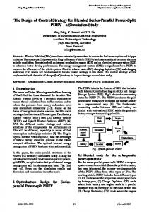
particularly in monitoring the climate [13]. The COSMIC-2 mission will have no CL observations, while either CYGNSS or ATOMMS will have ionospheric observations. Although the data volume of CL is much less than RO and GNSS reflections, it is still worthwhile to include CL in our OSSE study. By our test, the valid RO event between the similar LEOs (same inclination and orbit altitude) is few. We only consider the RO events between 24◦ /500 km LEOs and 72◦ /800 km LEOs in this study. The panel (g) of Fig. 2 shows the global distribution of the simulated daily RO events. The total RO number is ∼370 over here, and they mainly occur in the middle and the low latitude, where the orbits of low inclination LEO have intersection with that of high inclination LEO. The panel (h) shows the transionospheric trajectories of CL rays corresponding to the RO events in panel (g). Good coverage in the middle and the low latitude can be found. In addition, there is a little difference between the LEO-GNSS and LEO–LEO RO events. The speeds of LEO satellites are comparable, although their orbit altitudes might be different. Some LEO–LEO CL RO events can last a longer time and have a wider spatial coverage, particularly when two LEO satellites move in the similar direction. These will make the retrieval of the electron density profile less accurate, as we did for the GNSS RO using the Abel inversion based on the spherical symmetry assumption [34]. The same as the GNSS RO process, the electron densities at the tangent points for each CL ray are derived as the CL RO occultation results. As an example, we show such an example of the LEO–LEO CL RO event in Fig. 4. The panel (a) is the spatial coverage, and panel (b) is the simulated truth electron density profile along the tangent points by the IRI model and the corresponding Abel inversion. In this case, the extensions of the latitude and longitude of the tangent points from the top to the bottom are ∼ 45◦ and ∼ 60◦ , respectively. This case
3764
IEEE TRANSACTIONS ON GEOSCIENCE AND REMOTE SENSING, VOL. 52, NO. 7, JULY 2014
Fig. 4. (a) Coverage of the LEO orbits and ray tangent points and transionospheric trajectories of a typical LEO–LEO CL RO event. (b) Electron density profile of the simulated “truth” by IRI model and the Abel inversion corresponding to the RO event in panel (a).
lasts ∼18 min. The Abel-inverted electron density profile has significant deviation from the “truth.” Specifically, the peak density is significantly overestimated while the bottom density is underestimated, which result in the negative density below ∼250 km. It is due to the fact that the spherical symmetry assumption used in the Abel inversion is no longer correct over this larger area. Overall, the traditional used Abel inversion in GNSS RO retrieval is no longer applicable in CL RO. III. G LOBAL I ONOSPHERIC DATA A SSIMILATION M ODEL We developed a global ionospheric data assimilation model based on some previous studies [32], [33], [35], [37]. The key parameters of the model, including spatial and temporal resolutions, background and observation covariances, and background models, can be customized by the user. In this OSSE study, the selected background model is the IRI2007 model with the International Union of Radio Science (URSI) NmF2 and the Consultative Committee on International Radio (CCIR) hmF2 maps and the NeQuick topside option [3], [16]. The model grid spatial resolution is 2.5◦ in latitude and 5◦ in longitude and varies from 20 to 100 km in altitude from 80 to 2000 km with a linear transition. The plasmasphere above 2000 km is ignored in the simulation. There are totally ∼200 000 grid points globally. Fig. 5 gives a sketch map of the grid division of this data assimilation model. The background model error covariance is assumed to be the square of the background, and the error is spatially Gaussian correlated [32], [33]. Specifically, the correlation distance is two times larger in the daytime (12:00) than at night (00:00). The meridional correlation is larger in the middle latitude than both high and low latitudes. The typical value is 14◦ in 45◦ latitude and 8◦ in 0◦ and 85◦ latitudes. The zonal correlation distance linearly
Fig. 5. Sketch map of the grid division of the data assimilation model used in the OSSE study. Also, superimposed on the Earth’s surface is the IRI-modeled NmF2 (105 cm−3 ) under solar minimum (F10.7 = 75) in Autumn equinox.
increases from 10◦ in the equatorial area to 40◦ in the polar region. The vertical correlation exponentially increases from ∼50 km in 100-km altitude to ∼600 km in 2000-km altitude. The correlation distance is defined as the distance that the correlation coefficient of two grids decreases to be e−1/e (∼0.6922). The background model error covariance is set to 0 when the distance between two grid points is longer than
YUE et al.: OSSE STUDY ON IMAGING THE IONOSPHERE BY ASSIMILATING OBSERVATIONS
1000 km. The observation error is assumed to be uncorrelated. The error covariance of the background model and observations are assumed to be proportional to the square of their values, respectively [32]. The proportion coefficient is 0.1 and 0.01 for the model and observations, respectively, since we prefer to trust the observation more than the model. Please note that we give the same weight to each data type. In the real situation, the TEC error from the reflected signal is significantly larger than the direct signals, depending on the nadir antenna dimensions. We set the same observation error of RO and OR by assuming that the nadir antenna is large enough to ignore the precision difference between reflected and direct GNSS signals. The assimilation is performed using a Kalman filter method [35]–[37]. It is the standard Kalman filter except that the time forward of the covariance in the Kalman filter is not considered, which means that previous observations will have no effect on the current assimilation estimation. Therefore, the assimilation will obtain a global optimization by minimizing the difference between the model and the various observations. We carried out a series of simulation studies recently based on this model [35]–[37]. It is found that the global data assimilation can improve the Abel inversion and offers an optimal RO electron density profile retrieval if sufficient ROs are available. The observation operator is the integration along the ray path when the absolute slant TEC is assimilated. Duplicate rays, which pass through exactly the same grid points, are also removed. In addition, we have done a global ionospheric electron density reanalysis during 2002–2011 based on this model by assimilating almost all the available data, particularly LEO-based RO data, simultaneously [37]. The output of the reanalysis are 3-D gridded ionospheric electron densities with temporal and spatial resolutions of 1 h in universal time, 5◦ in latitude, 10◦ in longitude, and ∼30 km in altitude. Some preliminary validation studies show good improvements upon the IRI predictions. The main Kalman filter equation that we are going to solve is as follows: xa = xb + P H t [R + HP H t ]−1 (y − HXb )
(1)
where Xb and Xa are the prior and posterior background electron densities, respectively. P and R are the error covariances of the background model and observations, respectively. H and y are the observation operator and vector, respectively. In this OSSE study, the background grid point number is ∼200 000, and the simultaneously assimilated ray number can be up to ∼250 000 per hour after removing the duplicate rays. Ideally, the dimension of P , R, and H are 200 000 × 200 000, 250 000 × 250 000, and 250 000 × 200 000, respectively. At present, it is generally not possible to store all this information on a personal computer or workstation. Even using a supercomputer system, it is inefficient to do this computation. In this paper, we use the following assumptions and techniques to avoid the big storage and computation problems without the significant reduction of the assimilation accuracy. 1) Localization of the background and observation covariance: In this paper, the background covariance is assumed to be 0 when the distance between two grid points is larger than 1000 km, which is called covariance local-
3765
Fig. 6. Sketch map of the background covariance matrix distribution. The color represents the corresponding correlation coefficient.
ization. Covariance localization technique is usually used in the meteorology data assimilation system [4]. It is applicable to most systems because the correlation can be ignored when two grid points are spatially far away. The selection of ∼1000 km over here is based on both the computation capability and accuracy. The two grid points are assumed spatially Gaussian correlated with the correlation distance given earlier. In addition, when the correlation coefficient between two grids is less than 0.4, it will be ignored too. Fig. 6 gives a sketch map of the distribution and correlation coefficients of the covariance matrix. The grid points are arranged in longitude, latitude, and altitude directions sequentially. We can see that the matrix P is a sparse matrix after we made the aforementioned assumptions. We define the sparse ratio of a sparse matrix as follows: Sr = N(nonzero) /N(total)
(2)
where N(nonzero) and N(total) are the nonzero and the total element number of the matrix, respectively. The sparse ratio of our P in the study is ∼0.027% after we made covariance localization and correlation truncation. Regarding R, we assume the observation errors are uncorrelated, although the observation error from the same instrument might be correlated. Therefore, R is a diagonal matrix. For N observations, its sparse ratio is 1/N (∼0.0004% corresponding to 250 000 observations). 2) Use sparse matrix method for storage and calculation: A sparse matrix is a matrix populated primarily with zeros. As indicated earlier, both the background and observation error covariance matrix are “super” sparse. In addition, the observation operator H is also a sparse matrix since each ray only passes through a small number of the whole grid points. In this OSSE study, the average sparse
3766
IEEE TRANSACTIONS ON GEOSCIENCE AND REMOTE SENSING, VOL. 52, NO. 7, JULY 2014
Fig. 7. (a) Global 3-D of the simulated truth electron density, (b) the relative difference between the data assimilation background (a prior) model results and the simulated truth, and (c) the relative difference between the after data assimilation (a posterior) results with all available observing systems selected and the simulated truth during UT = 0 − 1 of the OSSE study.
ratio of the observation operator for all the rays from ground-based GNSS, LEO-GNSS RO, LEO-GNSS OR, and LEO–LEO CL is ∼0.0212%. When storing and manipulating sparse matrices on a computer, it is beneficial and often necessary to use specialized algorithms and data structures that take advantage of the sparse structure of the matrix [25], [26]. In our data assimilation system, we only store the nonzero elements of R, P , and H matrices in compressed-sparse-row format. Specifically, it only stores the nonzero element values, the corresponding column indexes, and row beginning indexes [25], [26]. This format is efficient for arithmetic operations, row slicing, and matrix–vector products. For these matrices stored in special sparse format, we use the corresponding algorithm to make the calculation, including transpose, addition, subtraction, multiplication, and division. 3) Iteration solving of the Kalman filter equation: Although we use the sparse matrix method in the storage and computation, it is still impossible to solve (1) directly when the matrix dimension is huge. One of the biggest computation challenges is the big matrix inverse. To avoid this problem, we suppose [R + HP H t ]−1 (y − HXb ) = T.
(3)
Therefore [R + HP H t ]T = y − Hxb .
(4)
Equation (4) is a sparse linear equation with huge unknown variables. Directly solving this equation is also inefficient. Many indirect methods, including conjugate gradient, semiiterative, successive overrelation, generalized minimal residual, etc., can be used [26]. For convergence during the iteration, some preconditioners like the Jacobi preconditioner, incomplete Cholesky factorization, incomplete lower triangular matrix-upper triangular matrix (LU) factorization, multigrid preconditioning can be used. Specifically, (4) will be solved via solving � � (5) C −1 [R + HP H t ]T − (y − Hxb ) = 0 where C is the preconditioner matrix. Depending on the computation capability and accuracy requirement, different combinations of iteration method and preconditioner can be used. IV. R ESULTS In this OSSE study, we group the observation system into six groups. They are as follows: ground-based GNSS observations, RO measurements from six 24◦ satellites, RO measurements from six 72◦ satellites, OR from six 24◦ satellites, OR from six 72◦ satellites, and CL between six 24◦ and six 72◦ satellites. The simulations for various kinds of combinations of these observation systems were performed. The time resolution of the data assimilation is ∼1 h. The total simulation time is one day. We use the NeQuick model driven by F10.7 = 110 to simulate
YUE et al.: OSSE STUDY ON IMAGING THE IONOSPHERE BY ASSIMILATING OBSERVATIONS
3767
Fig. 8. Magnetic local time and latitude variations of the error (in tecu) of the vertical TEC from the whole-day simulation for assimilating the following: (a) no data (a prior), (b) only CL, (c) only ground-based GNSS, (d) only ORs, (e) only GNSS RO, and (f) all the data.
the truth and the IRI2007 model driven by F10.7 = 150 as the background model in the assimilation. The NeQuick model uses the CCIR NmF2 and hmF2 maps and Epstein function to represent the altitude variation [16]. The 40 difference in the driven F10.7 index of two models is expected to be helpful in identifying the assimilation effect. The selected simulation day is Autumn equinox, September 23. For the ground-based GNSS observations, the time resolution varies from ∼1 s to 30 s. As for COSMIC-2, the time resolution is ∼1 s as designed. All the simulated observations with the corresponding time resolution will be assimilated into the model. However, in the data quality step, the duplicate ray links, which pass through the exact same grids, will be removed. Fig. 7 shows an example of the OSSE results during UT = 0 − 1. Panel (a) is the global 3-D electron density of the simulated truth, which is calculated by the NeQuick model driven by F10.7 = 110. Panel (b) shows the relative difference (%) of the data assimilation background model results, which is given by the IRI2007 model driven by F10.7 = 150, from the simulated truth. Panel (c) shows the relative difference of posterior results from the simulated truth. The shown case here assimilates all the observing systems (ground GNSS, RO, OR, and CL) simultaneously. Before the assimilation, the relative difference between the background and the simulated truth is significant and has obvious latitude, altitude, and local time variations due to the differences of the driving solar activity index and model architecture. The amplitudes of the relative
difference are concentrated in ∼50%–100%. However, after the assimilation, most relative differences reduce to ∼10%–30%. This demonstrates the validity of our model and algorithms. In some low altitude region with less data coverage, the difference is still significant. To illustrate the effect of the data volume, we plot the magnetic local time and latitude variations of the vertical TEC error (in tecu) to the simulated truth for assimilating no data, only CL, only ground-based GNSS, only OR (24◦ + 72◦ ), only GNSS RO (24◦ + 72◦ ), and all the data averaged for hourly assimilation over the one-day OSSE study in Fig. 8. As indicated, the vertical TEC error decreases significantly with the increase of the data volume. When only the CLs are assimilated, only the errors around the middle and low latitude regions are reduced a little in comparison with the prior. It is understandable because the CL between 24◦ and 72◦ LEO satellites mainly happens in the middle and the low latitude and has relative smaller data volume. We are not going to discuss the effect of CLs here since it is less effective than any other type of observations used in this OSSE. When only assimilating the ground-based GNSS, the assimilation error is reduced significantly except in southern middle and high latitude regions where less groundbased GNSSs are available. Please note that the ground-based GNSS already has a relatively higher horizontal resolution, which makes the ionospheric specification more reliable in terms of vertical TEC. Contrary to that of the ground-based GNSS, the error of only assimilating LEO-based OR is more
3768
IEEE TRANSACTIONS ON GEOSCIENCE AND REMOTE SENSING, VOL. 52, NO. 7, JULY 2014
with less or no GNSS stations, including ocean, polar region, middle and northern Africa, east Siberia, and western China, while for the situation of only assimilating LEO-based ORs, significant error mainly occurs over the middle of continuous land area, where no ORs can be observed as indicated in Fig. 2(f). Specifically, these areas include the middle of Oceania, north and south America, Africa, Asia, and Antarctica. The most significant error locates in the middle of Asia due to the larger and wider land. In low latitude ocean area (latitude < 30), the error is much less than that of higher latitude area because of the dense reflection coverage by the additional six low inclination satellites. When both ground GNSS and OR are assimilated simultaneously, the error is not significant anymore in either the land or the ocean area except the area with no ground GNSS coverage such as northern Africa and western China. To illustrate the different effects of the low (24◦ ) and high (72◦ ) inclination satellite constellations in specifying the ionosphere, we compare the daily average error of the vertical TEC in Fig. 10 among only assimilating 24◦ LEOs, 72◦ LEOs, and 24◦ + 72◦ LEOs for OR and RO, respectively. For both OR and RO, only assimilating six 24◦ satellites’ observations will mainly improve the low latitude (< 30◦ ) specification. There will be a global optimization if six 72◦ satellites’ observations are assimilated. The specification error in low latitude will be further reduced if six 24◦ in addition to six 72◦ satellites’ observations are assimilated simultaneously. The main difference between OR and RO is the larger error of OR over the middle land area. V. D ISCUSSION
Fig. 9. Longitude and latitude variations of the daily average error (in tecu) of the vertical TEC for the following: (a) Only assimilating ground-based GNSS, (b) only assimilating LEO-based ORs, and (c) assimilating both the ground GNSS and LEO-based ORs. Also, superimposed in panel (a) are the (•) GPS and (+) mixed GPS + GLONASS stations.
significant due to less ocean and, therefore, less OR in the northern hemisphere. When only the GNSS ROs are assimilated, the error is within ± 2 tecu. When all these data are assimilated simultaneously, all the errors are reduced to be within ± 1 tecu. As described in the observing system, the ground-based GNSS is expected to mainly provide the ionosphere information, particularly the horizontal resolution over the land, while the OR will focus on the ocean area. In Fig. 9, we compare the daily average error of the posterior in terms of vertical TEC between assimilating only ground-based GNSS, only OR, and both simultaneously. We can see clearly the error difference between the land and ocean areas in both situations. In the ocean–land transition area, the assimilation also shows less error due to the tilt feature of the GNSS ray and the effect of background correlation. When only ground-based GNSSs are assimilated, the significant error mainly happens in the area
In comparison with the LEO-GNSS RO method, the CL between LEO satellites gains significantly less RO events due to the slower relative movement between two LEO satellites. The average daily CL occultation number is ∼10 per 24◦ / 500 km–72◦ /800 km LEO satellite pair. This number is ∼30 per 800-km LEO satellite–GNSS satellite pair. In our simulation, only ∼30% of all CL RO events can be successfully retrieved by the Abel inversion because most CL RO has no integral coverage of the ionosphere below the LEO. As shown in Fig. 4, the Abel inversion error is significantly larger for some CL RO events due to the long lasting time and large drift of the RO tangent points. From the perspective of the ionospheric survey, the CL RO between LEOs has lower cost effect and accuracy in comparison with the GNSS signal-based RO. It should be pointed out that the LEO–LEO CL is mainly proposed for the lower atmosphere. Although the observation data volume is far less than that of the GNSS RO, it has a much higher accuracy, which makes significant sense for the climate monitoring [13]. In addition, it can observe more additional parameters such as ozone by transmitting specific radio wave frequency [17]. GNSS reflections have been widely studied to remotely sense the land, ocean, and ice since the accomplishment of the GPS system. Over the land area, the reflected GNSS signals can be used to derive the snow depth, soil moisture, vegetation growth, etc., through analyzing mainly the observed signalto-noise-ratio parameter [14], [15], [30]. In comparison with corresponding traditional observing methods, including both
YUE et al.: OSSE STUDY ON IMAGING THE IONOSPHERE BY ASSIMILATING OBSERVATIONS
3769
Fig. 10. Same as Fig. 9, but for the following: (a) ORs of six 24◦ satellites, (b) ORs of six 72◦ satellites, (c) ORs of six 24◦ + six 72◦ satellites, (d) ROs of six 24◦ satellites, (e) ROs of six 72◦ satellites, and (f) ROs of six 24◦ + six 72◦ satellites.
in situ and LEO-based remote sensing, the GNSS reflection technique has the advantages of sensing larger area and higher spatial and temporal resolutions by making use of the available global dense GNSS network. It is expected to complement the existing sensors. Through monitoring the global distribution and variability of soil moisture and snow, this technique will benefit the global water and carbon cycle studies, climate modeling, water supply management, drought and flood prediction, etc. However, ground GNSS reflections will always be treated as multipath and removed in ionospheric data process [27]. LEO-based ORs have been demonstrated to be useful in monitoring the mean sea level and ocean surface wind direction and speed [6], [9], [39]. However, more attention will need to be paid to the impact of GNSS ORs in monitoring the ionosphere, particularly the TEC along the GNSS ray. Marco-Pallares et al. [18] did a simulation study based on a single polar LEO satellite and showed that the GNSS reflections have big impact in ionospheric tomography imaging. As indicated by Figs. 9 and 10 in our OSSE study, there will be large specification error over the ocean area if only ground-based GNSSs are used in the assimilation. Significant error only occurs in the inland area if the ORs from six 72◦ inclination LEO satellites with spatially even distribution are used. Additional six 24◦ inclination LEO observations will further improve the specification in the low latitude region. Since the ocean area is ∼2.5 times more than that of the land, the effect of 12 LEO satellites’ OR is comparable or even better than that of the global groundbased GNSS stations in specifying the ionosphere from a global
scale. When both the ground-based GNSS and LEO OR are assimilated simultaneously, the two can complement each other very well and mitigate most errors. Please note that we did not consider the reflections from the ice, which could be useful in specifying the polar region. Overall, the LEO-based GNSS OR technique offers us a potential valuable way to monitor the ocean area ionosphere and is worthy of further study. The ionosphere has obvious regional features such as equatorial ionization anomaly (EIA), middle latitude trough, Weddell sea anomaly, longitudinal variations, etc. These OR observations will complement ground- and LEO-based techniques over the ocean and therefore benefit both the ionospheric scientific research and application. As indicated from our simulation, when either the OR or RO from only the six 72◦ inclination satellites is assimilated, the ionosphere specification will be generally optimized globally, with relatively larger error in the EIA region because of larger gradients of electron density over there. While only six 24◦ satellites’ observations are assimilated, there will be significant specification error over the middle and the high latitude area due to less or no sampling over there. The specification error is larger, particularly in the southern American area, due to the higher geographic latitude location of EIA here. When both the 24◦ and 72◦ satellites have simultaneous observations, the two can complement each other well and give a global optimization of the ionosphere specification. As an example, we plot the daily latitude distribution (in percentage) of the RO number (a) and OR number (b) for only six 24◦ satellites, only six 72◦
3770
IEEE TRANSACTIONS ON GEOSCIENCE AND REMOTE SENSING, VOL. 52, NO. 7, JULY 2014
Fig. 11. Latitude distribution in percentage (%) of the (a) RO events and (b) ORs observed by (- -) six 24◦ satellites, (-.) six 72◦ satellites, and (-) both. The latitude bin size is 5◦ .
Fig. 12. Global mean error in terms of vertical TEC (tecu) for only assimilating ROs from 24◦ , 72◦ , and 24◦ + 72◦ satellites, respectively.
satellites, and both, respectively, in Fig. 11. We can see that the 24◦ satellites will enhance the observation in the low latitude very much. The OR has more observations in the southern hemisphere than the northern hemisphere. To quantify the effect of both constellations in specifying the ionosphere, we calculate the global average error of vertical TEC for assimilating only 24◦ , 72◦ , and 24◦ + 72◦ satellites, respectively, in Fig. 12. Only RO results are given here as an example. OR will show the similar conclusion. When only six 24◦ satellites’ observations are used, the global mean error is ∼2.6 tecu, while it is ∼1.3 tecu for 72◦ inclination satellites. When both are assimilated simultaneously, the error will be reduced to ∼0.5 tecu. Please note that the statistical numbers shown here are mainly used to demonstrate the relative effects of different LEO constellations. The assimilation error in the real situation should be larger due to observation uncertainties and model deviations. In addition, the COSMIC-2 will also have another two additional payloads named the RF Beacon and the Velocity, Ion Density and Irregularities [40]. These two will provide in situ and nadir integrated ionospheric information, which is expected to be useful in global ionospheric specification too. Further OSSE studies are needed to evaluate their relative importance. In this OSSE study, we use an empirical model as the background of the data assimilation. Therefore, this study cannot account for the effect of some small scale ionospheric variations that are not captured by the IRI model. It is also not suitable to evaluate the effect of these observing systems in short term forecasting the ionosphere. The ionosphere is a very complicated system owing to the coupling of different physical, chemical, and dynamic processes with the background neutral atmosphere, magnetosphere, and lower thermosphere. It is controlled by a variety of factors, including the solar UV/EUV
radiation, the neutral backgrounds (winds, compositions, temperatures, tides, etc.), electric field in low and high latitudes, magnetosphere energy input in the polar region, tides and planetary waves in the lower boundary, and some instability processes inside. Up to date, there is no essentially ionospheric short-term forecast capability in the community because of the following: 1) The ionosphere has a relatively shorter memory to the past because the ionosphere is controlled very much by the multiple external drivers; 2) few observations of ionospheric drivers are available, particularly in real time; and 3) no perfect operational model of this complicated system is available. Although space weather monitoring and prediction was paid much attention by humans recently, it is still impossible to measure and predict all those ionospheric drivers to predict the ionosphere and thermosphere system. Fortunately, the most important parameter of this system, electron density, has been widely observed by different ground- and spacebased techniques. Now, the community has formed many global ionospheric electron density networks, including ionosondes, incoherent scatter radars, ground-based GNSS, satellite in situ measurement, LEO-based GNSS, etc. Most of these data are publicly available even in near real time. Important physical, chemical, dynamic, and coupling processes will result in various forms of variability in ionospheric electron density. Aside from driving the theoretical model by as much real data as possible, another potential way that can enhance the shortterm forecast capability is trying to optimize those ionospheric drivers by assimilating electron density observations based on their correlations [32], [33], [41], [42]. The most frequently used assimilation method is called ensemble Kalman filter [32], [41], [42]. As indicated in this study, the COSMIC-2 mission will provide incredible observation number with good spatial and temporal coverage globally for the first time. By combining
YUE et al.: OSSE STUDY ON IMAGING THE IONOSPHERE BY ASSIMILATING OBSERVATIONS
traditional ground-based observations with those satellite observations, the community is approaching the ionosphere prediction further. VI. C ONCLUSION The main points of this paper include the following. 1) A flexible global ionospheric data assimilation model based on the IRI and Kalman filter is constructed. The huge computation and storage problems are militated through the localization of the error covariance and the use of the sparse matrix method and iteration solving method. Previous and current studies show that this model is stable and computation efficient [35]–[37]. 2) An OSSE has been done based on the real IGS global ground GNSS network, the planned COSMIC-2 mission orbits, and real GPS and GLONASS orbits. Specifically, the COSMIC-2 will have six LEO satellites in ∼500-km altitude with 24◦ inclination and another six satellites in ∼800-km altitude with 72◦ inclination. The simulated measurements include the slant TEC of groundbased GNSS, RO between COSMIC-2 LEO and GPS/GLONASS satellites, ORs from COSMIC-2 LEO satellites, and CLs between COSMIC-2 low and high inclination satellites. A variety of simulations have been done by combining different observations. The NeQuick model is used to simulate the measurements. 3) The ORs show great impact in specifying the ionosphere except over the inland area. It complements the existing ground-based GNSS network, which mainly observes the ionosphere over the land area. The 24◦ and 72◦ satellites can complement each other to optimize the global ionospheric specification. 4) The simulations results show that the COSMIC-2 observations would be expected to contribute significantly to the accurate ionosphere nowcast. Further studies are needed to demonstrate its effects in predicting the ionosphere in short term.
ACKNOWLEDGMENT The ground international global navigation satellite system (GNSS) service data and GNSS orbits used in this study are acquired as part of NASA’s Earth Science Data Systems and archived and distributed by the CDDIS (ftp://cddis.gsfc.nasa.gov). R EFERENCES [1] E. S. Andreeva, “Radio tomographic reconstruction of ionization dip in the plasma near the Earth,” J. Exp. Theor. Phys. Lett., vol. 52, no. 3, pp. 142–148, Aug. 1990. [2] J. R. Austen, S. J. Franke, and C. H. Liu, “Ionospheric imaging using computerized tomography,” Radio Sci., vol. 23, no. 3, pp. 299–307, May/Jun. 1988. [3] D. Bilitza and B. W. Reinisch, “International reference ionosphere 2007: Improvements and new parameters,” Adv. Space Res., vol. 42, no. 4, pp. 599–609, Aug. 2008. [4] F. Bouttier and P. Courtier, “Data assimilation concepts and methods,” in Meteorological Training Course Lecture Notes. Reading, U.K.: Eur. Cent. Med.-Range Weather Forecasts, 1999, Presentation.
3771
[5] G. S. Bust and C. N. Mitchell, “History, current state, and future directions of ionospheric imaging,” Rev. Geophys., vol. 46, no. 1, pp. RG1003-1– RG1003-23, Mar. 2008. [6] M. P. Clarizia, C. P. Gommenginger, S. T. Gleason, M. A. Srokosz, C. Galdi, and M. Di Bisceglie, “Analysis of GNSS-R delay-Doppler maps from the UK-DMC satellite over the ocean,” Geophys. Res. Lett., vol. 36, no. 2, pp. L02608-1–L02608-5, Jan. 2009. [7] E. J. Fremouw, J. A. Secan, and B. M. Howe, “Application of stochastic inverse theory to ionospheric tomography,” Radio Sci., vol. 27, no. 5, pp. 721–732, Sep./Oct. 1992. [8] C. J. Fong, W. T. Shiau, C. T. Lin, T. C. Kuo, C. H. Chu, S. K. Yang, N. L. Yen, S. S. Chen, Y. H. Kuo, Y. A. Liou, and S. Chi, “Constellation deployment for the FORMOSAT-3/COSMIC mission,” IEEE Trans. Geosci. Remote Sens., vol. 46, pt. 1, no. 11, pp. 3367–3379, Nov. 2008. [9] J. L. Garrison, A. Komjathy, V. Zavorotny, and S. J. Katzberg, “Wind speed measurement using forward scattered GPS signals,” IEEE Trans. Geosci. Remote Sens., vol. 40, no. 1, pp. 50–65, Jan. 2002. [10] G. A. Hajj, R. Ibanez-Meier, E. R. Kursinski, and L. J. Romans, “Imaging the ionosphere with the global positioning system,” Int. J. Imaging Syst. Technol., vol. 5, no. 2, pp. 174–184, Summer 1994. [11] B. M. Howe, K. Runciman, and J. A. Secan, “Tomography of the ionosphere: Four-dimensional simulations,” Radio Sci., vol. 33, no. 1, pp. 109–128, Jan./Feb. 1998. [12] A. Komjathy, B. Wilson, X. Pi, V. Akopian, M. Dumett, B. Iijima, O. Verkhoglyadova, and A. J. Mannucci, “JPL/USC GAIM: On the impact of using COSMIC and ground-based GPS measurements to estimate ionospheric parameters,” J. Geophys. Res., vol. 115, no. A2, pp. A02307-1– A02307-10, Feb. 2010. [13] E. R. Kursinski, D. Ward, A. Otarola, R. Frehlich, C. Groppi, S. Albana, M. Shein, W. Bertiger, H. Pickett, and M. Ross, New Horizons in Occultation Research: Studies in Atmosphere and Climate. Berlin, Germany: Springer-Verlag, 2009, ch. 5, pp. 295–313. [14] K. M. Larson, E. Gutmann, V. Zavorotny, J. Braun, M. Williams, and F. G. Nievinski, “Can we measure snow depth with GPS receivers?” Geophys. Res. Lett., vol. 36, no. 7, pp. L17502-1–L17502-, Sep. 2009. [15] K. M. Larson, J. Braun, E. E. Small, V. U. Zavorotny, E. Gutmann, and A. L. Bilich, “GPS multipath and its relation to near-surface soil moisture content,” IEEE J. Sel. Topics Appl. Earth Observ. Remote Sens., vol. 3, no. 1, pp. 91–99, Mar. 2010. [16] R. Leitinger, S. Radicella, and B. Nava, “Electron density models for assessment studies—New developments,” Acta. Geod. Hung., vol. 37, no. 2/3, pp. 183–193, Jan. 2002. [17] M. S. Lohmann, A. S. Jensen, H.-H. Benzon, and A. S. Nielsen, “Application of window functions for full spectrum inversion of cross-link radio occultation data,” Radio Sci., vol. 41, no. 3, pp. RS3001-1–RS3001-19, Jun. 2006. [18] J. Marco-Pallares, G. Ruffini, and L. Ruffini, “Ionospheric tomography using GNSS reflections,” IEEE Trans. Geosci. Remote Sens., vol. 43, no. 2, pp. 321–326, Feb. 2005. [19] C. Noll, “The crustal dynamics data information system: A resource to support scientific analysis using space geodesy,” Adv. Space Res., vol. 45, no. 12, pp. 1421–1440, Jun. 2010. [20] R. J. Norman, P. L. Dyson, E. Yizengaw, J. L. Marshall, C. S. Wang, B. A. Carter, D. Wen, and K. Zhang, “Radio occultation measurements from the Australian microsatellite FedSat,” IEEE Trans. Geosci. Remote Sens., vol. 50, no. 11, pp. 4832–4839, Nov. 2012. [21] S. E. Pryse and L. Kersley, “A preliminary experimental test of ionospheric tomography,” J. Atmos. Terr. Phys., vol. 54, no. 7, pp. 1007–1012, Jul./Aug. 1992. [22] T. D. Raymund, J. R. Austen, S. J. Franke, C. H. Liu, J. A. Klobuchar, and J. Stalker, “Application of computerized-tomography to the investigation of ionospheric structures,” Radio Sci., vol. 25, no. 5, pp. 771–789, Sep./Oct. 1990. [23] A. D. Richmond, E. C. Ridley, and R. G. Roble, “A thermosphere/ ionosphere general circulation model with coupled electrodynamics,” Geophys. Res. Lett., vol. 19, no. 6, pp. 601–604, Mar. 1992. [24] C. Rocken, Y.-H. Kuo, W. Schreiner, D. Hunt, S. Sokolovskiy, and C. McCormick, “COSMIC system description,” Terr. Atmos. Ocean. Sci., vol. 11, no. 1, pp. 21–52, Mar. 2000. [25] Y. Saad, “SPARSKIT: A basic tool kit for sparse matrix computations,” Res. Inst. for Adv. Comput. Sci., NASA Ames Res. Center, Moffett Field, CA, USA, Tech. Rep. RIACS90-20, 1990. [26] Y. Saad, Iterative Methods for Sparse Linear Systems. Philadelphia, PA, USA: SIAM, 2003. [27] S. Schaer, “Mapping and predicting the Earth’s ionosphere using the Global Positioning System,” Ph.D. dissertation, Astron. Inst., Univ. of Bern, Bern, Switzerland, 1999.
3772
IEEE TRANSACTIONS ON GEOSCIENCE AND REMOTE SENSING, VOL. 52, NO. 7, JULY 2014
[28] W. S. Schreiner, X. Yue, Y.-H. Kuo, D. Mamula, and D. Ector, “Satellite constellations for space weather and ionospheric studies: Status of the COSMIC and planned COSMIC-2 missions, Presentation,” in Proc. 9th Space Weather Workshop 92nd AMS Annu. Meet., New Orleans, LA, USA, 2012, pp. 1–16. [29] R. W. Schunk, L. Scherliess, J. J. Sojka, D. C. Thompson, D. N. Anderson, M. Codrescu, C. Minter, T. J. Fuller-Rowell, R. A. Heelis, M. Hairston, and B. M. Howe, “Global Assimilation of Ionospheric Measurements (GAIM),” Radio Sci., vol. 39, no. 1, pp. RS1S02-1– RS1S02-11, Feb. 2004. [30] E. E. Small, K. M. Larson, and J. Braun, “Sensing vegetation growth using reflected GPS signals,” Geophys. Res. Lett., vol. 37, no. 12, pp. L12401-1– L12401-5, Jun. 2010. [31] C. Wang, G. Hajj, X. Pi, I. G. Rosen, and B. Wilson, “Development of the global assimilative ionospheric model,” Radio Sci., vol. 39, no. 1, pp. RS1S06-1–RS1S06-11, Feb. 2004. [32] X. Yue, W. Wan, L. Liu, F. Zheng, J. Lei, B. Zhao, G. Xu, S.-R. Zhang, and J. Zhu, “Data assimilation of incoherent scatter radar observation into a one-dimensional midlatitude ionospheric model by applying ensemble Kalman filter,” Radio Sci., vol. 42, no. 6, pp. RS6006-1–RS6006-20, Dec. 2007. [33] X. Yue, W. Wan, L. Liu, and T. Mao, “Statistical analysis on spatial correlation of ionospheric day-to-day variability by using GPS and incoherent scatter radar observations,” Ann. Geophys., vol. 25, no. 8, pp. 1815–1825, Aug. 2007. [34] X. Yue, W. S. Schreiner, J. Lei, S. V. Sokolovskiy, C. Rocken, D. C. Hunt, and Y.-H. Kuo, “Error analysis of Abel retrieved electron density profiles from radio occultation measurements,” Ann. Geophys., vol. 28, no. 1, pp. 217–222, Jan. 2010. [35] X. Yue, W. S. Schreiner, Y.-C. Lin, C. Rocken, Y.-H. Kuo, and B. Zhao, “Data assimilation retrieval of electron density profiles from radio occultation measurements,” J. Geophys. Res., vol. 116, no. A3, pp. A03317-1– A03317-12, Mar. 2011. [36] X. Yue, W. S. Schreiner, and Y.-H. Kuo, “A feasibility study of the radio occultation electron density retrieval aided by a global ionospheric data assimilation model,” J. Geophys. Res., vol. 117, no. A8, pp. A08301-1– A08301-9, Aug. 2012. [37] X. Yue, W. S. Schreiner, Y.-H. Kuo, D. C. Hunt, W. Wang, S. C. Solomon, A. G. Burns, D. Bilitza, J.-Y. Liu, W. Wan, and J. Wickert, “Global 3-D ionospheric electron density reanalysis based on multisource data assimilation,” J. Geophys. Res., vol. 117, no. A9, pp. A09325-1– A09325-17, Sep. 2012. [38] X. Yue, W. S. Schreiner, C. Rocken, Y.-H. Kuo, and J. Lei, “Artificial ionospheric wave number 4 structure below the F2 region due to the Abel retrieval of radio occultation measurements,” GPS Sol., vol. 16, no. 1, pp. 1–7, Jan. 2012. [39] C. Zuffada, T. Elfouhaily, and S. Lowe, “Sensitivity analysis of wind vector measurements from ocean reflected GPS signals,” Remote Sens. Environ., vol. 88, no. 3, pp. 341–350, Dec. 2003. [40] FORMOSAT-7/COSMIC-2 spacecraft science payloads to spacecraft bus interface requirement document, COSMIC, Boulder, CO, USA, FS7-IRD0002. [Online]. Available: http://www.docstoc.com/docs/137235787/ 110408_Science_PL_to_SC_IRD_for_public_release [41] T. Matsuo and E. A. Araujo-Pradere, “Role of thermosphere-ionosphere coupling in a global ionospheric specification,” Radio Sci., vol. 46, no. 6, pp. RS0D23-1–RS0D23-7, Dec. 2011. [42] L. Scherliess, D. C. Thompson, and R. W. Schunk, “Ionospheric dynamics and drivers obtained from a physics-based data assimilation model,” Radio Sci., vol. 44, no. 1, pp. RS0A32-1–RS0A32-8, Feb. 2009.
Xinan Yue received the Ph.D. degree in space physics from the Graduate School of Chinese Academy of Sciences, Beijing, China, in 2008. He is a Project Scientist in the University Corporation for Atmospheric Research (UCAR) Constellation Observing System for Meteorology, Ionosphere, and Climate Program Office and responsible for the ionospheric data process and evaluation. His scientific interests include ionospheric/thermospheric modeling, data assimilation, global navigation satellite system applications, remote sensing, and space weather. He has published nearly 60 science citation index (SCI) papers as either first author or coauthor in related fields.
William S. Schreiner received the Ph.D. degree in aerospace engineering sciences from the University of Colorado at Boulder, Boulder, CO, USA, in 1993. He has been with the University Corporation for Atmospheric Research (UCAR), Boulder, CO, USA, since then. He is the Manager of the Constellation Observing System for Meteorology, Ionosphere, and Climate (COSMIC) Data Analysis and Archive Center at UCAR. His research focuses on global-navigation-satellite-system data processing with special emphasis on radio-occultation applications, satellite precise orbit determination, atmospheric and ionospheric remote sensing, and processing and modeling of geodetic observations. He is currently working on the design, development, and operation of a COSMIC-2 mission that is scheduled to launch in 2016.
Ying-Hwa Kuo received the Ph.D. degree from the Penn State University, Pennsylvania, USA, in 1983. He has been with the University Corporation for Atmospheric Research (UCAR)/National Center for Atmospheric Research (NCAR) since then. He is the Director of the Constellation Observing System for Meteorology, Ionosphere, and Climate Project at UCAR, Boulder, CO, USA. He is also a Senior Scientist at the Mesoscale and Microscale Meteorology Division of NCAR. He has been responsible for the development and applications of the NCAR Fifth Generation Mesoscale Model and, more recently, the Weather Research and Forecasting model. He is also serving as the National Director for the Developmental Testbed Center, a multiple-agency funded center with the primary mission of research to operation transition in numerical weather prediction. He has served as NCAR advisor for more than 20 Ph.D. students and has published more than 120 journal papers. His scientific interest includes mesoscale modeling, hurricanes, mesoscale convective systems, GPS meteorological applications, and data assimilation.
John J. Braun received the B.A. degree in physics and mathematics from the University of Colorado at Boulder, Boulder, CO, USA, and the PhD. degree from the Department of Aerospace Engineering Sciences, University of Colorado at Boulder, in 2004. He is a Project Scientist with the University Corporation for Atmospheric Research Constellation Observing System for Meteorology, Ionosphere, and Climate Program Office where he is leading the ground-based research activities of the group. His research interests include remote sensing of the Earth and its atmosphere using global navigation satellite systems, the water cycle, and improving observations for atmospheric data assimilation applications.
Yu-Cheng Lin received the M.S. degree from National Central University (NCU), Taiwan, in 2006. He is currently a Software Engineer of the Constellation Observing System for Meteorology, Ionosphere, and Climate (COSMIC) Project at the University Corporation for Atmospheric Research, Boulder, CO, USA. He began working on global navigation satellite system and low-Earth-orbit data processing for ionospheric studies when he was a graduate student of the Institute of Space Science, NCU. After getting his M.S. degree from NCU, he worked at the Taiwan Analysis Center for COSMIC in the Taiwan Central Weather Bureau, where he integrated various scientific data processing software from both U.S. and Taiwanese research communities into production environment. He joined the COSMIC Project in 2010.
YUE et al.: OSSE STUDY ON IMAGING THE IONOSPHERE BY ASSIMILATING OBSERVATIONS
Weixing Wan graduated from Wuhan University, Wuhan, China, in 1982 and received the M.S. and Ph.D. degrees from the Wuhan Institute of Physics, Chinese Academy of Sciences (CAS), Wuhan, in 1984 and 1990, respectively. He is the Director of the Key Laboratory of Ionospheric Environment, Institute of Geology and Geophysics, CAS, Beijing. He has a broad interest in ionospheric physics and radio wave propagation. His research mainly focuses on the following: regional properties of ionospheric disturbances; coupling process of the ionospheric and the lower atmosphere; ionospheric storms and space weather; and ionospheric climatology and modeling. He has served as a member of multiple domestic/international committees and a principle investigator/coinvestigator of many projects from the National Science Foundation of China, State High-Tech Development Plan (863), National Basic Research Program (973), CAS, and other funding agencies. He has been the superior for nearly 30 Ph.D. and master students and published ∼260 SCI papers. He contributed significantly to the research development of ionosphere and thermosphere in China through training the young scientist and developing the observing system. He was elected as the Academician of CAS in 2011.
3773