Hindawi Publishing Corporation Mathematical Problems in Engineering Volume 2015, Article ID 293176, 9 pages http://dx.doi.org/10.1155/2015/293176
Research Article Obtaining Cross Modal Similarity Metric with Deep Neural Architecture Ruifan Li,1,2 Fangxiang Feng,1 Xiaojie Wang,1,2 Peng Lu,1 and Bohan Li1 1
School of Computers, Beijing University of Posts and Telecommunications, Beijing 100876, China Engineering Research Center of Information Networks, Ministry of Education, Beijing 100876, China
2
Correspondence should be addressed to Ruifan Li;
[email protected] Received 14 September 2014; Accepted 24 December 2014 Academic Editor: Florin Pop Copyright © 2015 Ruifan Li et al. This is an open access article distributed under the Creative Commons Attribution License, which permits unrestricted use, distribution, and reproduction in any medium, provided the original work is properly cited. Analyzing complex system with multimodal data, such as image and text, has recently received tremendous attention. Modeling the relationship between different modalities is the key to address this problem. Motivated by recent successful applications of deep neural learning in unimodal data, in this paper, we propose a computational deep neural architecture, bimodal deep architecture (BDA) for measuring the similarity between different modalities. Our proposed BDA architecture has three closely related consecutive components. For image and text modalities, the first component can be constructed using some popular feature extraction methods in their individual modalities. The second component has two types of stacked restricted Boltzmann machines (RBMs). Specifically, for image modality a binary-binary RBM is stacked over a Gaussian-binary RBM; for text modality a binarybinary RBM is stacked over a replicated softmax RBM. In the third component, we come up with a variant autoencoder with a predefined loss function for discriminatively learning the regularity between different modalities. We show experimentally the effectiveness of our approach to the task of classifying image tags on public available datasets.
1. Introduction Recently, there is a growing demand for analyzing the complex systems with great number of variables [1, 2], such as multimodal data with image and text, due to the availability of computational power and massive storage. For one thing, information often naturally comes in multiple modalities of a large number of variables. For example, a travel photo shared on the website is usually tagged with some meaningful words. For another, analyzing those heterogeneous data of great number of variables from multiple sources could benefit different modalities. For instance, speaker’s articulation and muscle movement can often aid in disambiguating between speeches with similar phones. During the past few years, motivated by the biological propagation phenomena in distributed structure of human brain, deep neural learning has received considerable attention from the year of 2006. These deep neural learning methods are proposed to learn hierarchical and effective representations to facilitate various tasks with respect to recognizing and analyzing in complex artificial system. Even
with only a very short development, deep neural learning has achieved great success in some tasks of modeling the single modal data, such as speech recognition systems [3–6] and computer vision systems [7–12], to name a few. Motivated by the progress in deep neural learning, in this paper, we endeavor to construct a computational deep architecture for measuring the similarity between modalities in complex multimodal system with a large number of variables. Our proposed framework, bimodal deep architecture (BDA), has three closely consecutive components. For images and text modalities, the first component can be constructed by some popular feature extraction methods in each individual modality. The second component has two types of stacked restricted Boltzmann machines (RBMs). Specifically, for image modality a Bernoulli-Bernoulli RBM (BB-RBM) is stacked over an RBM; for text modality a BBRBM is stacked over a replicated softmax RBM (RS-RBM). In the third component, we come up with a variant autoencoder with a predefined loss function for discriminatively learning the regularity hidden within modalities.
2
Mathematical Problems in Engineering
It is worthwhile to highlight several aspects of the BDA proposed in this paper. (i) In the first component of the BDA, for image modality, three methods are utilized in our setting. However, we could explore more feature extraction methods. (ii) In the second component of the BDA, we stack two RBMs for each modality. In theory, we could stack more RBMs to make a more effective representation. (iii) In the third component of the BDA, motivated by the deep neural architecture, we come up with a loss function to keep small distance for semantically similar bimodal data and to generate large distance for semantically dissimilar ones. (iv) The work in this paper primarily focuses on the image and text bimodal data. However, the BDA presented here can be naturally extended to other different bimodal data. The remainder of this paper is organized as follows. Section 2 describes and discusses the related work. Section 3 presents our deep architecture and its learning algorithm. Section 4 introduces the datasets, describes the other two methods for comparisons, and reports the experimental results. Finally Section 5 draws the conclusion and discusses the future work.
2. Related Work There have been several approaches to learning from cross modal data with many variables. In particular, Blei and Jordan [13] extend latent Dirichlet allocation (LDA) by mining the topic-level relationship between images and text annotations. Xing et al. [14] build a joint model to integrate images and text, which can be viewed as an undirected extension to LDA. Jia et al. [15] proposes a combination of the undirected Markov random field and the directed LDA. However, this type of models with a single hidden layer is unable to obtain efficient representations because of the complexity of images and text. Recently, motivated by deep neural learning, Chopra et al. [16] propose to learn a function such that the norm in the embedded space approximates the semantic distance. This learned network, however, keeps only half of the structure and only fits for unimodal data. Ngiam et al. [17] use a deep autoencoder for vision and speech fusion. Srivastava and Salakhutdinov [18] develop a deep Boltzmann machine as a generative model for images and text. However, these two works focus on cross modal retrieval but not the similarity metric. Another line of research focuses on bimodal semantic hashing, which tries to represent data as binary codes. Subsequently, Hamming metric is applied for the learned codes as the measure of similarity. McFee and Lanckriet [19] propose a framework based on multimodal kernel learning approaches. However, this framework is limited to linear projections. Most similar to our work, Masci et al. [20] propose a framework based on the neural autoencoder
to merge multiple modalities into a single representation space. However, this framework can only be used for labeled bimodal data.
3. BDA for Cross Modal Similarity The main idea of our deep framework is to construct hierarchical representations of bimodal data. This framework, as shown in Figure 1, has three closely consecutive components. In the first component, the low-level representations by classical single-modal methods for these two types of data are obtained, respectively. For images, the features are extracted by four descriptors in MPEG-7, and gist features are combined to form the low-level representations. For tag words, the typical bag-of-words (BOW) model is used for low-level representations. In the second component, the low-level representations usually with different dimensions for image and tag words are distilled to form the mid-level representations using two stacked restricted Boltzmann machines (RBMs), respectively. The first layer RBMs, a Gaussian RBM for low-level representation of the images and a replicated softmax for those of text, are adopted mainly for normalizing these bimodal data with the same output units. The second layer RBMs, two binary RBMs, are used for expecting more abstract representations. In the third component, we propose a variant of autoencoder for learning the high-level semantic similar/dissimilar representations of these bimodal data. The details of this network are described in Section 3.3. All numbers in the boxes are the number of neurons used in each layer. The detailed description of each component is presented in the following sections. In the training stage, a collection of pairs of image and text is presented to the system. As a result, by our learning algorithm the system could learn the neural connection weights. In the test stage, a new pair of bimodal data is shown to the learned system such that we can obtain the similarity/dissimilarity between the pair of unseen data. 3.1. Obtaining Basic Representations. Different unimodal data, such as images or text, usually have different methods to extract the representative features. We use these extracted features as our basic representations. For image modality some popular methods, such as MPEG-7 and gist descriptors, can be used. Gist represents the dominant spatial structure of a scene by a set of perceptual dimensions, including naturalness, openness, roughness, expansion, and ruggedness. These perceptual dimensions can be estimated using spectral and coarsely localized information. One part of MPEG-7 is a standard for visual descriptors. We use four different visual descriptors defined in MPEG-7 for image representations: color layout (CL), color structure (CS), edge histogram (EH), and scalable color (SC). CL is based on spatial distribution of colors and is obtained by applying the DCT transformation. CS is based on color distribution and local spatial structure of the color. EH is based on spatial distribution of edges. SC is based on the
Mathematical Problems in Engineering
3
Code layer
1704
1024
1024
1024
1024
BB-RBM
BB-RBM
Decoder
Decoder
1024
1024
512
512
GB-RBM
RS-RBM
Encoder
Encoder
1704
4000
1024
1024
4000 BoW
MPEG-7 gist
Bus red bus Double twostory decker Windows Windshield Wet ground Basic level
Advanced level
Intermediate level
Figure 1: A deep framework is used for measuring the similarity of cross modal data such as images and text. From left to right, first, the classical methods for each modality could be used to extract basic modality-specific features. For example, we use MPEG-7, Gist, and some known features descriptors for images; we use bag-of-words model for tags. Second, for each modality two RBMs are stacked for extracting intermediate modality-specific features. For images, we stack a binary RBM over a Gaussian RBM; for text, we stack a binary RBM over a replicated softmax. Third, an autoencoder with similar constraint is used for extracting similar presentations. The number in each box is the neurons adopted in this layer.
color histogram in HSV color space encoded by a Haar transformation. For text modality, we use the classical bag-of-words model for its basic representations. A dictionary of 𝐾 highfrequency words is built from all the words in the database. Then, each tag can be represented as a multinomial variable. Conveniently, 1-of-𝐾 coding scheme is adopted. Thus, the tags of an image could be represented as a vector with 𝐾 one/zero elements, in which each element stands for whether the tag is in the dictionary or not. For tags in the dictionary, they are encoded as 1s, and vice versa. 3.2. Learning Intermediate Representations 3.2.1. Modeling Binary Data. For binary data, as in the second layer of the second component in our framework, we use RBMs for modeling them. An RBM [21] is an undirected graphical model with stochastic binary units in the visible layer and the hidden layer but without connections between units within these two layers. Given that there are 𝑛 visible units k and 𝑚 hidden units h, and each unit is distributed by Bernoulli distribution with logistic activation function 𝜎(𝑥) = 1/(1 + exp(−𝑥)), we then define a joint probabilistic distribution 𝑝 over the visible units k and hidden units h 1 (1) exp (−𝐸 (k, h)) , 𝑍 in which 𝑍 is the normalization constant and 𝐸(k, h) is the energy function defined by the configurations of all the units as 𝑝 (k, h) =
𝑛 𝑚
𝑛
𝑚
𝑖=1 𝑗=1
𝑖=1
𝑗=1
𝐸 (k, h) = −∑∑𝑤𝑖𝑗 V𝑖 ℎ𝑗 − ∑𝑏𝑖 V𝑖 − ∑𝑐𝑗 ℎ𝑗 .
(2)
Here, 𝑤𝑖𝑗 is the connection weight between the 𝑖th visible unit with state V𝑖 and the 𝑗th hidden unit ℎ𝑗 with state V𝑗 . And the
two parameters, 𝑏𝑖 and 𝑐𝑗 , are biases for the 𝑖th visible unit and the 𝑗th hidden unit, respectively. 3.2.2. Modeling Real-Valued Data. We model the image features with real-valued data, as in the first layer of the second component in our framework, using Gaussian RBM. It is an extension of the binary RBM replacing the Bernoulli distribution with Gaussian distribution for the visible data [22]. The energy function of different configurations of visible units and hidden ones is 2
𝑛 𝑚
𝑛 𝑚 (V − 𝑏 ) V 𝐸 (k, h) = −∑∑𝑤𝑖𝑗 𝑖 ℎ𝑗 + ∑ 𝑖 2 𝑖 − ∑𝑐𝑗 ℎ𝑗 , 𝜎𝑖 2𝜎𝑖 𝑖=1 𝑗=1 𝑖=1 𝑗=1
(3)
in which 𝜎𝑖 is the variance of the Gaussian distribution of 𝑖th visible unit. And we usually set the variances 𝜎𝑖 equal to one for all visible units. Except the variance 𝜎𝑖 , the other parameters in the above equation have the same meanings as those in (2). 3.2.3. Modeling Count Data. For the text features with count data, as in the first layer of the second component in our framework, we use replicated softmax model [23] for modeling these sparse vectors. The energy function of the date configurations is defined as follows: 𝑛 𝑚
𝑛
𝑚
𝑖=1 𝑗=1
𝑖=1
𝑗=1
𝐸 (k, h) = −∑∑𝑤𝑖𝑗 V𝑖 ℎ𝑗 − ∑𝑏𝑖 V𝑖 − 𝑀∑ 𝑐𝑗 ℎ𝑗 ,
(4)
where 𝑀 is the total number of words in a document. And the other parameters in the above equation have the same meanings as those in (2). Note that this replicated softmax model can be interpreted as an RBM model that uses a single visible multinomial unit with support 1, . . . , 𝐾 which is sampled 𝑀 times.
4
Mathematical Problems in Engineering
In the second component of our framework, for each modality we stack two RBMs to learn the intermediate representations. These two-layer stacked RBMs can be trained by the greedy layer-wise training method [24, 25]. And we can efficiently learn all the above three kinds of RBMs by using the contrastive divergence (CD) approximation [26]. 3.3. Learning Advanced Representations. In the third component of our framework, we propose a special type of autoencoder for bimodal representations to learn the similarity. As shown in the rightmost of Figure 1, this autoencoder consists of two subnets, in which each subnet is fully connected perceptron. And these two networks are connected by some predefined similarity measure on the code layer. By designing a proper loss function from energy-based learning paradigm [27], we could learn the similar representations of these two bimodalities. Formally, we denote the mapping from the inputs of two subnets to the code layers as 𝑓(𝑝; W𝑓 ) and 𝑔(𝑞; W𝑔 ), in which 𝑓(⋅) is for the image modality and 𝑔(⋅) is for the text modality. Here, 𝑝 and 𝑞 denote one intermediate representation for image and one intermediate representation for a given tag. And W denotes the weight parameters in these two subnets. The subscripts 𝑓 and 𝑔 of the weight W denote the corresponding two modalities, respectively. We define the compatibility measure between 𝑖th pair of image 𝑝𝑖 and its given tags 𝑞𝑖 as 𝐶 (𝑝𝑖 , 𝑞𝑖 ; W𝑓 , W𝑔 ) = 𝑓 (𝑝𝑖 ; W𝑓 ) − 𝑔 (𝑞𝑖 ; W𝑔 )2 ,
(5)
where ‖ ⋅ ‖2 is the L2 norm. To learn the similar representations of these two modalities for one object, we come up with a loss function given input 𝑝𝑖 , 𝑞𝑖 , and a binary indicator 𝛿 with respect to the inputs. In our settings, the indictor variable 𝛿 equals one if the tag words 𝑞𝑖 correspond to the image 𝑞𝑖 , and the indictor variable 𝛿 equals zero otherwise. To simplify the notation we group the network parameters W𝑓 and W𝑔 into one parameter Θ. As a result, we define the loss function ℓ on any pair of inputs 𝑝𝑖 and 𝑞𝑖 as ℓ (𝑝𝑖 , 𝑞𝑖 , 𝛿; Θ) = 𝛼 (ℓ𝑓 (𝑝𝑖 ; W𝑓 ) + ℓ𝑔 (𝑞𝑖 ; W𝑔 )) + (1 − 𝛼) ℓ𝑐 (𝑝𝑖 , 𝑞𝑖 , 𝛿; Θ) ,
(6)
where 2 ℓ𝑓 (𝑝𝑖 ; W𝑓 ) = 𝑝𝑖 − 𝑝̂𝑖 2 ,
(7a)
2 ℓ𝑔 (𝑞𝑖 ; W𝑔 ) = 𝑞𝑖 − 𝑞̂𝑖 2 ,
(7b)
ℓ𝑐 (𝑝𝑖 , 𝑞𝑖 , 𝛿; Θ) = 𝛿𝐶2 + (1 − 𝛿) exp(−𝜆𝐶) .
(7c)
Here, the total loss comprises of three parts. The first two losses ℓ𝑓 and ℓ𝑔 are caused by data reconstruction errors for the given inputs (an image and its tags) of two subnets, while the third loss ℓ𝑐 (𝑝𝑖 , 𝑞𝑖 , 𝛿; Θ), called the contrastive loss, is incurred by whether the image and tags are compatibility or not in two different situations indicated by 𝛿. And ‖ ⋅ ‖2
in (7a) and (7b) denotes the L2 norm. The 𝑝̂𝑖 in (7a) is the construction representation of the input image 𝑝𝑖 , and the 𝑞̂𝑖 in (7b) is the construction representation of the input text 𝑞𝑖 . 𝜆 in (7c) is a constant, which depends on the upper bound of 𝐶(𝑝𝑖 , 𝑞𝑖 ; Θ) on all training data. The constant 𝛼 (0 < 𝛼 < 1) in the total loss function (6) is a parameter used to trade off between two groups of losses, the reconstruction losses, and the compatibility loss. By the standard backpropagation algorithm [28] we can learn the connections weights among neurons in this autoencoder. During learning, the two subnets are coupled at their code layer with the similarity measure. After being learned, the two subnetworks will have different parameters even if they have the same architecture. As a result, the codes for new inputs can be obtained using the learned network parameters. To summarize, by the above three consecutive components we can learn the similarity metric for bimodal data.
4. Experiments and Results We evaluate our proposed method for the task of image annotation selection compared with multilayer perceptron (MLP) with two hidden layers and canonical correlation analysis (CCA) with RBMs as a benchmark method on two publicly available datasets. In the following sections, we will describe the two datasets used, our experimental settings, and the evaluation criteria. Moreover, we report and discuss our experimental results. 4.1. Datasets and Preprocessing. The two datasets used in our experiments are the Small ESP Game dataset [29] and the multimodal learning challenge 2013 (MLC-2013) dataset [10]. The ESP dataset, briefly known as ESP, was created by Luis von Ahn using crowdsourcing efforts of ESP online players from different locations. Specifically, the ESP consists of 100,000 labeled images with the corresponding labeled tags. The images in the ESP have a variety of sizes; the tags are influenced by the game format. Note that each image in the ESP only has the correct tag words. Some examples from the ESP are shown in Figure 2. The ESP dataset is available at http://www.cs.cmu.edu/∼biglou/resources/. The MLC-2013 dataset, briefly known as MLC, was created by Ian J. Goodfellow for the workshop on representation learning at International Conference on Machine Learning, ICML 2013. Specifically, the MLC consists of 1,000 manually labeled images, which were obtained by Google image search queries for some of the most commonly used words in the ESP. And for each image, two labels are given; one fits better than the other. The labels were intended to resemble those in the EPS. For example, they include incorrect spellings that were common in the EPS. Some examples from the MLC are shown in Figure 3. The MLC dataset is available at http://www-etud.iro.umontreal.ca/∼goodfeli/mlc2013.html. In all our experiments, we use the ESP as the training set and the MLC as the test set. In addition, we note that each image in the ESP involves a unique group of tags; we must firstly construct the counterpart group of tags for each
Mathematical Problems in Engineering
Knife slice war cut Missile sharp brown Black rocket silver White missile bomb Bombs ad poster loaf
Computer Record Stack dvd 4x case Disc blue
5
27 speed Speed limit post Limit sky please Green mph Grass white
Mobile Remote Buttons Cell Black Case Call Screen Cellphone
Medicine warning Red drug pregnant Not sign do Ear label blue
Tall future clouds Building sky water Rocket sea hotel Skyscraper cloud white Blue space point
Figure 2: Examples from the ESP dataset. The top is images and the bottom is their corresponding group of tag words. See text for more details.
Word Control Channel Changer Volume Zapper On Off Change
Word Flower Flowers Daisies Blue Stem Petal Petals White Yellow
Tree Nature Leaves Green White Man Stubble Person Elf Gnome Acorn Hand Holding Orange
Man Tree Blond People Path Hill Nature Face Green
Figure 3: Two examples from the MLC dataset. Each one shows the image and its two tags. The words in sky blue box are from its original tag, and the words in carnation box are from the generated one.
image in the ESP. Therefore, in order to train our system, we automatically generate an incorrect counterpart for word tags of each image in the ESP. This can be achieved by randomly choosing one from all the correct tag words of the rest of the images, while ensuring that each of the tag words occurs only one time. That is our preprocessing procedure. 4.2. Settings of Our BDA Method. In this section, we describe the settings in our experiments, including the details of feature extraction methods in the first component and the neurons configurations in the second and third components.
In the first component, for image modality, three popular methods are adopted. The first group of features is obtained by the following steps: (1) preprocess images using local contrast normalization [30]; (2) train a 𝐾-means dictionary on patches of ESP; (3) extract soft threshold features [31] from all image patches and then downsample using local max pooling; (4) train a 𝐾-means dictionary on patches of these 𝐾-means feature maps; (5) extract a second layer of soft threshold features, using global max pooling to make a “bag of visual words” (BOVW) feature vector for each image. The second group of features is obtained by MPEG-7 visual descriptors. We use 192 coefficients of DCT transformation for Cl, 256 coefficients form for CS, fixed 80 coefficients for EH, and 256 coefficients form for CS. The software module based on the MPEG-7 Reference Software (available at http://www.cs.bilkent.edu.tr/∼bilmdg/bilvideo-7/Software .html) permits obtaining all four different descriptors. Thus, we obtain the features of MPEG-7 descriptors with the size of 784. The third group of features is obtained by gist descriptor. The package used in our paper is available at http://people .csail.mit.edu/torralba/code/spatialenvelope/ for downloading. Through all the three groups of features, each image is represented as a vector of 1704 dimensions. More specifically, this image representation is composed of the leading 408 dimensions from BOVW, the middle 784 dimensions from MPEG-7, and the last 512 dimensions from gist features. For text representation we use bag-of-words model. In our experiments, a dictionary of 4000 high-frequency words is built from all the tag words of ESP. Thus, each tag is represented as a vector with 4000 one/zero elements. In the second component, we use the neurons configuration of 1704-1024-1024 for image modality and of 40001024-1024 for text modality. That is, Gaussian-Bernoulli RBM has the 1704 visible neurons and 1024 hidden neurons. The replicated softmax has 4000 visible neurons and 1024 hidden neurons. And the two Bernoulli RBMs in the above layers in the intermediate representations have 1024 visible neurons and 1024 hidden neurons. In the third component, we use the neurons configuration of 1024-512 both for image modality and text modality. That
6 is, the autoencoders in the advanced representations for both modalities have 1024 visible neurons and 512 hidden neurons. As for the parameters, we illustrate the method for setting the parameter 𝛼 in the following section. We have mentioned that the parameter 𝜆 depends on the upper bound of 𝐶(𝑝𝑖 , 𝑞𝑖 ; Θ) on all training data in the previous section. Practically, we repeated several experiments with different values for choosing this parameter. Then, the value of 0.1 is set for this parameter. 4.3. Settings of Benchmark Methods. For comparison of two benchmark methods, MLP with two hidden layers and CCA with RBMs are used in our experiments. Next, we describe the details of these two methods. The MLP is a popular supervised learning model in artificial neural networks system [32]. In our experiments, we use the neural structure proposed in [10]. This network has the following structure. The input layer of this network is the basic representation for the image modality. Two hidden layers with the same number of neurons are utilized. The top layer is the basic representation for the text modality. To be specific, we set the input layer of the MLP system to have 1704 neurons and the output layer to have 4000 neurons. And each of two hidden layers has 1024 neurons. And all the neurons in this MLP have logistic activation function. This MLP system is graphically depicted in Figure 4. To test an unseen image, we first use the preprocessing modules outside the dashed box to obtain the bimodal representations. Then, using the learned system, we can obtain the output as the basis for judging the better fitting tag words. The idea behind this design is to model the nonlinear mapping directly from the image modality to the text modality. Note that, unlike the traditional MLP, the MLP used in our experiments has two hidden layers. And this MLP with multiple hidden layers can be seen as a kind of deep neural architecture, which would benefit the nonlinearly semantic mapping from one modality to the other. The CCA [33, 34] is a multivariate statistical model that facilitates the study of linear interrelationships between two groups of variables. More specifically, given a pair of data 𝑝 and 𝑞, the CCA attempts to discover matrices 𝑈 and 𝑉 such that 𝑈𝑝 and 𝑉𝑞 have maximum correlations. The first 𝑑 canonical components of 𝑈 and 𝑉 could be used for projecting an unseen pair of data into a 𝑑-dimensional space. The CCA-based system for modeling the relationship between multimodal data achieves the state-of-art performance in analyzing numerous cross modal tasks. To name a few, recent work [17, 35, 36] shows the strength of CCA system. Therefore, we adopt a CCA system as one of our benchmark systems. In the CCA system, the two groups of variables are modal representations. One group of input of the CCA system is the basic representation for the image modality. The other is the replicated softmax RBM representation based on the BOW model. Then, the CCA is applied for these two quantities. To be specific, we set the image representation to have 1,704 neurons. And a replicated softmax RBM is used with an input of 4,000 neurons and output of 1,024 neurons. The canonical
Mathematical Problems in Engineering
1024
4000
RS-RBM
BoW 1024
Bus red bus Double twostory decker Windows Windshield Wet ground
1024
1704
MPEG-7 gist
Figure 4: The MLP system used in our experiments. In the lower right corner, an image is represented using MPEG-7 and gist descriptors forming a vector with 1,704 neurons. And in the upper right corner, the corresponding tag words are first represented using the BOW model. Furthermore, a replicated softmax RBM with 4,000 visible neurons and hidden 1,024 neurons is adopted to learn a text representation. Finally, in the dashed box, from the bottom to the top, an MLP with two hidden layers is designed to learn the mapping from image modality to text modality.
components 𝑑 in CCA is set as 1,024. This CCA system is graphically depicted in Figure 5. To test an unseen image, we first use the preprocessing modules outside the dashed box to obtain the bimodal representations. Then, using the learned mapping, we can obtain the output as the basis for judging the better fitting tag words. The CCA code is available at http://davidroihardoon.com/Professional/Code.html. 4.4. Evaluation Criteria. The performance of predictions of a classifier is evaluated based on the accuracy. Here, the accuracy is, for simplicity, defined as the area under the receiving operating curve (ROC). The adoption of this accuracy is motivated by two facts. One is its successful application on evaluating binary classifiers [37]. The other is the encouragement by the builder of the MLC dataset [10]. Next, we will describe the definition and its computation of the accuracy used for evaluating these models. Often used for evaluating binary classifiers, the ROC is a plot of false positive rate 𝑈1 (𝑡) at a decision threshold 𝑡 on the 𝑥-axis against true positive rate 𝑈0 (𝑡) at 𝑡 on the 𝑦-axis. And the subscript for 𝑈 denotes the corresponding class. Given the score output of a classifier, an instance is classified as the positive class if the score is greater than the decision threshold 𝑡 or as the negative otherwise. Note that these two quantities 𝑈1 (𝑡) and 𝑈0 (𝑡) will be monotonically nondecreasing with increasing 𝑡. We then define the accuracy as follows: 1
+∞
0
−∞
Accuracy ≜ ∫ 𝑈0 (𝑠) 𝑑𝑈1 (𝑠) = ∫
𝑈0 (𝑠) 𝑢1 (𝑠) 𝑑𝑠,
(8)
Mathematical Problems in Engineering Table 1: Accuracies achieved by BDA and benchmark methods.
1024
1024
1024
GB-RBM
RS-RBM
1704
4000
MPEG-7 gist
BoW
Method BDA CCA [17] MLP [10]
0.9
Bus red bus Double twostory decker Windows Windshield Wet ground
0.7 0.6
0.4
in which 𝑢1 (⋅) is the density function for class 1. Thus, 𝑈1 (𝑡) = 𝑡 ∫−∞ 𝑢1 (𝑠)𝑑𝑠 = 𝑃 (𝑠 ≤ 𝑡 | 1) is the false positive rate at threshold 𝑡. When dealing with empirical distributions the integral is replaced by the sum. In [37], an efficient algorithm is proposed for calculating the accuracy. In order to fulfill the computation, the three models in our experiments should be able to produce a continuous valued output that can be used for ranking its predictions. Therefore, we define the continuous valued output 𝑃(𝑝𝑖 ) for the positive class as the ratio of the squared compatibility metric of an image 𝑝𝑖 with its true tag words 𝑞𝑖 to the sum of the squared compatibility metrics of an image 𝑝𝑖 with its two tag words 𝑞𝑖 and 𝑞̃𝑖 . To be specific, the value 𝑃(𝑝𝑖 ) is defined as follows: 𝐶2 (𝑝𝑖 , 𝑞𝑖 ) . 𝐶2 (𝑝𝑖 , 𝑞𝑖 ) + 𝐶2 (𝑝𝑖 , 𝑞̃𝑖 )
0.8
0.5
Figure 5: The CCA system used in our experiments. From the lower left corner, the image modality is represented using MPEG-7 and gist descriptors forming a vector with size 1,704. Then, a Gaussian RBM with 1,704 visible neurons and 1,024 hidden neurons is used to learn the image representation. From the lower right corner, the text modality is represented using BoW model forming a vector with size 4000. Then, a replicated softmax RBM with 4,000 visible neurons and hidden 1,024 neurons is adopted to learn a text representation. Finally, a CCA model with 1,024 twin inputs and 1,024 twin outputs is built using these bimodal representations.
𝑃 (𝑝𝑖 ) ≜
Accuracy (%) 88.96 85.54 81.54
1
Accuracy
1024
7
(9)
4.5. Results. We compare our deep neural architecture with an MLP-based system with two hidden layers and a CCAbased system with two RBMs used. The experimental results of different methods are shown in Table 1. Our BDA achieves the highest accuracy of 88.96% among the three models. And the CCA-based system gains better performance than that of the MLP-based system. Besides, we investigate the effect of hyperparameter 𝛼 in loss function (6). Figure 6 shows the accuracies achieved of different values of 𝛼, by setting 𝛼 from 0.0 to 1.0 with 0.1 as the step size. As shown in this figure, the best performance
0
0.2
0.4
0.6
0.8
1
𝛼
Figure 6: The effect of hyperparameter 𝛼 on our system.
is achieved when the value of 𝛼 is equal to 0.4. Note that, when the value of 𝛼 is set to 1, the BDA degenerates to two autoencoders resulting in an accuracy with random guess; when the value of 𝛼 is set to 0, the BDA degenerates to an only one autoencoder, with a higher accuracy than that of a random guess. 4.6. Discussion. In this section we will make a discussion on the three methods and the experimental results. The models used in our experiments have something in common. Firstly, for image modality, some popular descriptors are adopted. And for the text modality, we adopt the classical BOW model. These low-level modal specific representations are substantially built for further more abstract representations. Secondly, all the three models obtain a cross modal metric enabling these heterogeneous data from different sources to be comparable. Note that the experimental results are largely affected by the differences among these models. In the MLP-based system, the nonlinear mapping function is obtained directly from the low-level representation of image modality to that of text modality. The assumption behind the MLP-based system is that the text representation is abstract whilst the image representation is concrete, relatively. In contrast, the other two systems, the CCA-based and our BDA-based system, treat the bimodal data as the same starting point. The assumption behind these systems is that there exists a common representation space for bimodal data of one object. Recent neurobiological research [38] has a strong support for the latter. Therefore, the BDA-based and CCA-based systems outperform the MLP-based system. Furthermore, note that the CCA only considers the linear coefficient, whilst our BDA uses the nonlinear reconstruction and compatibility constraints. Some important information related to these two modalities cannot be captured by the CCA method. Overall, the accuracies achieved by the three models are expected.
8 The experiments on the hyperparameter 𝛼 show that the BDA relates to the unimodal autoencoder, as already shown in the above experimental results. And also it is interesting to note that the highest accuracy is not achieved at the medium value of 0.5. It means that the bimodal autoencoder in the BDA system primarily keeps the reconstructions of modality-specific data and secondly considers the compatibility between modalities. This could be used as a guideline for heuristically setting the hyperparameter 𝛼.
5. Conclusion To conclude, we propose a computational deep neural architecture for measuring the similarity between different modalities in complex system with image and text. Our proposed framework closely combines feature extraction methods for individual modality and deep neural networks using stacked RBMs and a variant of neural autoencoder architecture. We show experimentally the effectiveness of our approach to the task of classifying image tags on public available datasets. Our computational framework is flexible and could be extended in several ways. For example, we could explore more feature extraction methods in the first component. As another example, complex neural based representation could be exploited. Moreover, this architecture presented here can be naturally extended to other different modalities. In our future work we will investigate this flexibility in other complex systems.
Conflict of Interests The authors declare that there is no conflict of interests regarding the publication of this paper.
Acknowledgments This work was partially supported by National Natural Science Foundation of China (nos. 61273365, 61100120, 61202247, and 61202248), National High Technology Research and Development Program of China (no. 2012AA011103), Discipline Building Plan in 111 Base (no. B08004), and Fundamental Research Funds for the Central Universities (no. 2013RC0304). The authors would also like to thank the editor and the anonymous reviewers for their useful comments and suggestions that allowed them to improve the final version of this paper.
References [1] L. Li, H. Peng, J. Kurths, Y. Yang, and H. J. Schellnhuber, “Chaosorder transition in foraging behavior of ants,” Proceedings of the National Academy of Sciences, vol. 111, no. 23, pp. 8392–8397, 2014. [2] Y. Bengio, “Learning deep architectures for AI,” Foundations and Trends in Machine Learning, vol. 2, no. 1, pp. 1–27, 2009. [3] K. Chen and A. Salman, “Learning speaker-specific characteristics with a deep neural architecture,” IEEE Transactions on Neural Networks, vol. 22, no. 11, pp. 1744–1756, 2011.
Mathematical Problems in Engineering [4] A.-R. Mohamed, G. E. Dahl, and G. Hinton, “Acoustic modeling using deep belief networks,” IEEE Transactions on Audio, Speech and Language Processing, vol. 20, no. 1, pp. 14–22, 2012. [5] G. Heigold, V. Vanhoucke, A. Senior et al., “Multilingual acoustic models using distributed deep neural networks,” in Proceedings of the 38th IEEE International Conference on Acoustics, Speech, and Signal Processing (ICASSP ’13), pp. 8619–8623, IEEE Computer Society, Vancouver, Canada, May 2013. [6] D. Yu, L. Deng, and F. Seide, “The deep tensor neural network with applications to large vocabulary speech recognition,” IEEE Transactions on Audio, Speech and Language Processing, vol. 21, no. 2, pp. 388–396, 2013. [7] G. E. Hinton and R. R. Salakhutdinov, “Reducing the dimensionality of data with neural networks,” Science, vol. 313, no. 5786, pp. 504–507, 2006. [8] H. Lee, R. Grosse, R. Ranganath, and A. Y. Ng, “Unsupervised learning of hierarchical representations with convolutional deep belief networks,” Communications of the ACM, vol. 54, no. 10, pp. 95–103, 2011. [9] A. Krizhevsky, I. Sutskever, and G. Hinton, “Imagenet classification with deep convolutional neural networks,” in Advances in Neural Information Processing Systems, vol. 25, pp. 1106–1114, Morgan Kaufmann, Lake Tahoe, Nev, USA, 2012. [10] I. J. Goodfellow, D. Erhan, P. L. Carrier et al., “Challenges in representation learning: a report on three machine learning contests,” in Proceedings of the 20th International Conference on Neural Information Processing, pp. 117–124, IEEE Computer Society, Daegu, Korea, 2013. [11] C. Farabet, C. Couprie, L. Najman, and Y. Lecun, “Learning hierarchical features for scene labeling,” IEEE Transactions on Pattern Analysis and Machine Intelligence, vol. 35, no. 8, pp. 1915–1929, 2013. [12] F. Feng, X. Wang, and R. Li, “Cross-modal retrieval with correspondence autoencoder,” in Proceedings of the 22nd ACM International Conference on Multimedia, pp. 7–16, ACM, Orlando, Fla, USA, 2014. [13] D. M. Blei and M. I. Jordan, “Modeling annotated data,” in Proceedings of the 26th Annual International ACM SIGIR Conference on Research and Development in Information Retrieval, pp. 127–134, ACM, New York, NY, USA, 2003. [14] E. P. Xing, R. Yan, and A. G. Hauptmann, “Mining associated text and images with dual-wing harmoniums,” in Proceedings of the 21st Annual Conference on Uncertainty in Artificial Intelligence (UAI ’05), pp. 633–641, AUAI Press, Arlington, Va, USA, July 2005. [15] Y. Jia, M. Salzmann, and T. Darrell, “Learning cross-modality similarity for multinomial data,” in Proceedings of ACM the International Conference on Multimedia Information Retrieval, pp. 2407–2414, IEEE, Washington, DC, USA, November 2011. [16] S. Chopra, R. Hadsell, and Y. LeCun, “Learning a similarity metric discriminatively, with application to face verification,” in Proceedings of the IEEE Computer Society Conference on Computer Vision and Pattern Recognition (CVPR ’05), pp. 539– 546, IEEE, Washington, DC, USA, June 2005. [17] J. Ngiam, A. Khosla, M. Kim, J. Nam, H. Lee, and A. Y. Ng, “Multimodal deep learning,” in Proceedings of the 28th International Conference on Machine Learning, pp. 689–696, Omnipress, Bellevue, Wash, USA, July 2011. [18] N. Srivastava and R. Salakhutdinov, “Multimodal learning with deep Boltzmann machines,” in Advances in Neural Information Processing Systems, vol. 25, pp. 2231–2239, Morgan Kaufmann, Lake Tahoe, Nev, USA, 2012.
Mathematical Problems in Engineering [19] B. McFee and G. Lanckriet, “Learning multi-modal similarity,” Journal of Machine Learning Research, vol. 12, no. 8, pp. 491–523, 2011. [20] J. Masci, M. M. Bronstein, A. M. Bronstein, and J. Schmidhuber, “Multimodal similarity-preserving hashing,” IEEE Transactions on Pattern Analysis and Machine Intelligence, vol. 36, no. 4, pp. 824–830, 2014. [21] P. Smolensky, “Information processing in dynamical systems: foundations of harmony theory,” in Parallel Distributed Processing: Explorations in the Microstructure of Cognition, D. E. Rumelhart, J. L. McClelland, and C. PDP Research Group, Eds., vol. 1, pp. 194–281, MIT Press, Cambridge, Mass, USA, 1986. [22] M. Welling, M. Rosen-Zvi, and G. Hinton, “Exponential family harmoniums with an application to information retrieval,” in Advances in Neural Information Processing Systems 17, pp. 501– 508, Morgan Kaufmann, Vancouver, Canada, 2004. [23] R. Salakhutdinov and G. Hinton, “Replicated softmax: an undirected topic model,” in Advances in Neural Information Processing Systems, vol. 22, pp. 1607–1614, Morgan Kaufmann, Vancouver, Canada, 2009. [24] G. E. Hinton, S. Osindero, and Y. W. Teh, “A fast learning algorithm for deep belief nets,” Neural Computation, vol. 18, no. 7, pp. 1527–1554, 2006. [25] Y. Bengio, P. Lamblin, D. Popovici, and H. Larochelle, “Greedy layer-wise training of deep networks,” in Advances in Neural Information Processing Systems 19, pp. 153–160, MIT Press, Vancouver, Canada, 2007. [26] G. E. Hinton, “Training products of experts by minimizing contrastive divergence,” Neural Computation, vol. 14, no. 8, pp. 1771–1800, 2002. [27] Y. LeCun, S. Chopra, R. Hadsell, M. Ranzato, and F.-J. Huang, “A tutorial on energy-based learning,” in Predicting Structured Data, G. Bakir, T. Hofman, B. Sch¨olkopf, A. Smola, and B. Taskar, Eds., pp. 1–59, MIT Press, Cambridge, Mass, USA, 2006. [28] D. E. Rumelhart, G. E. Hinton, and R. J. Williams, “Learning internal representations by error propagation,” Nature, vol. 323, no. 6088, pp. 533–536, 1986. [29] L. von Ahn and L. Dabbish, “Labeling images with a computer game,” in Proceedings of the SIGCHI Conference on Human Factors in Computing Systems, pp. 319–326, ACM Press, Vienna, Austria, 2004. [30] N. Pinto, D. D. Cox, and J. J. DiCarlo, “Why is real-world visual object recognition hard?” PLoS Computational Biology, vol. 4, no. 1, article e27, 2008. [31] A. Coates and A. Y. Ng, “The importance of encoding versus training with sparse coding and vector quantization,” in Proceedings of the 28th International Conference on Machine Learning (ICML ’11), pp. 921–928, Bellevue, Wash, USA, July 2011. [32] F. M. Ham and I. Kostanic, Principles of Neurocomputing for Science and Engineering, McGraw-Hill Higher Education, 1st edition, 2000. [33] T. W. Anderson, An Introduction to Multivariate Statistical Analysis, John Wiley and Sons, New York, NY, USA, 3rd edition, 2003. [34] D. R. Hardoon, S. Szedmak, and J. Shawe-Taylor, “Canonical correlation analysis: an overview with application to learning methods,” Neural Computation, vol. 16, no. 12, pp. 2639–2664, 2004. [35] N. Rasiwasia, J. C. Pereira, E. Coviello et al., “A new approach to cross-modal multimedia retrieval,” in Proceedings of the 18th
9 ACM International Conference on Multimedia, pp. 251–260, ACM, New York, NY, USA, 2010. [36] J. Kim, J. Nam, and I. Gurevych, “Learning semantics with deep belief network for cross-language information retrieval,” in Proceedings of the 24th International Conference on Computational Linguistics, pp. 579–588, ACL Press, IIT Bombay, India, 2012. [37] T. Fawcett, “An introduction to ROC analysis,” Pattern Recognition Letters, vol. 27, no. 8, pp. 861–874, 2006. [38] S. V. Shinkareva, V. L. Malave, R. A. Mason, T. M. Mitchell, and M. A. Just, “Commonality of neural representations of words and pictures,” NeuroImage, vol. 54, no. 3, pp. 2418–2425, 2011.
Advances in
Operations Research Hindawi Publishing Corporation http://www.hindawi.com
Volume 2014
Advances in
Decision Sciences Hindawi Publishing Corporation http://www.hindawi.com
Volume 2014
Journal of
Applied Mathematics
Algebra
Hindawi Publishing Corporation http://www.hindawi.com
Hindawi Publishing Corporation http://www.hindawi.com
Volume 2014
Journal of
Probability and Statistics Volume 2014
The Scientific World Journal Hindawi Publishing Corporation http://www.hindawi.com
Hindawi Publishing Corporation http://www.hindawi.com
Volume 2014
International Journal of
Differential Equations Hindawi Publishing Corporation http://www.hindawi.com
Volume 2014
Volume 2014
Submit your manuscripts at http://www.hindawi.com International Journal of
Advances in
Combinatorics Hindawi Publishing Corporation http://www.hindawi.com
Mathematical Physics Hindawi Publishing Corporation http://www.hindawi.com
Volume 2014
Journal of
Complex Analysis Hindawi Publishing Corporation http://www.hindawi.com
Volume 2014
International Journal of Mathematics and Mathematical Sciences
Mathematical Problems in Engineering
Journal of
Mathematics Hindawi Publishing Corporation http://www.hindawi.com
Volume 2014
Hindawi Publishing Corporation http://www.hindawi.com
Volume 2014
Volume 2014
Hindawi Publishing Corporation http://www.hindawi.com
Volume 2014
Discrete Mathematics
Journal of
Volume 2014
Hindawi Publishing Corporation http://www.hindawi.com
Discrete Dynamics in Nature and Society
Journal of
Function Spaces Hindawi Publishing Corporation http://www.hindawi.com
Abstract and Applied Analysis
Volume 2014
Hindawi Publishing Corporation http://www.hindawi.com
Volume 2014
Hindawi Publishing Corporation http://www.hindawi.com
Volume 2014
International Journal of
Journal of
Stochastic Analysis
Optimization
Hindawi Publishing Corporation http://www.hindawi.com
Hindawi Publishing Corporation http://www.hindawi.com
Volume 2014
Volume 2014