Oceanographic Applications of Remote Sensing - CiteSeerX

*

Chapter IV-A-3 in CRC Press Book Entitled “Oceanographic Applications of Remote Sensing”

-

(Ed’s) Ikeda, M. and Dobson, F.

AIRBORNE AND SATELLTTE SAR INVESTIGATIONS OF SEA-ICE SURFACE CHARACTERISTICS Mark R. Drinkwater Jet Propulsion Laboratory California Institute of Technology 4800 Oak Grove Drive Pasadena CA 91109 a.

INTRODUCTION

b. SAR AND THE STUDY OF SEA ICE i, From Seasat to the Present Day ii. ERS -1 Validation Experiments c. CM-WAVELENGTHS i.

AND SEA ICE GEOPHYSICS

Impact of Frequency ~icmw~ of IV@WWQS

ii, Polarization Diversity between w~ m Sea-Ice ~

. .

.

iii. Snowcover: A thermal insulator and microwave blanket Snow Frost FIowxs iv. Seasonal Considerations v. Validation Measurements and Surface Proof d. MICROWAVE SCA’ITERING MODELS AND INVERSION e. DISCUSSION AND CONCLUSIONS f. ACKNOWLEDGEMENTS g. BIBLIOGRAPHY h. FIGURE CAPTIONS

a.

INTRODUCTION

The logistical difficulty of making measurements in polar oceans during winter makes remote-sensing techniques attractive. Microwave synthetic aperture radar (SAR) offers day and night imaging, without impact from atmospheric conditions. SAR satellite receiving stations located in Fairbanks, Alaskw Troms@, Norway; Kiruna, Sweden; West Freugh, Scotland; and Prince Albert and Gatineau, Canada, form a chain of station receiving masks which cover all but the Eastern Arctic basin. Similar Antarctic stations are operated by the Germans at the Chilean General Bemardo OHiggins base; and by the Japanese at Syowa [1]. A further Antarctic station is currently being built at the US. McMurdo base [2] to be operational in 1995-96, and will complete coverage of the Southern Ocean around the Antarctic continent. This hi-polar network forms the basis for over a decade of continuous satellite observations of the polar ice cover. Sea ice plays a key role in climate through its interactions with and feedbacks to the atmosphere and ocean [3]. As ice covers on average 107o of the global ocean area (rising to a maximum of 13$ZO) this high-albedo insulating layer acts as an intermediary in the way in which the local atmosphere and ocean communicate. Sea-ice characteristics reflect and respond to the balance of fluxes of momentum, heat, water vapour and salt at the ocean surface, by adjustments in thickness and salinity disrnbution. Through surface albedo and the fraction of leads, ice surface conditions impact the net heat flux at the surface. Similarly, winter sea-ice growth prwonditions the mixed layer, due to salinization by salt rejection [4]. It influences global ocean characteristics from the perspective of participating in formation of water masses such as Antarctic bottom water or the high salinity shelf water found along the shelves of the Weddell and Ross Seas [5] and the Beaufort and Chukchi Seas. Thus sea ice has an important impact beyond locally regulating the exchange of heat, momentum and water vapour between ocean and atmosphere. In recent years SAR evolved and matured into an operational tool [6], but the data have barely been exploited to their full scientific potential. This chapter points toward some of the insight SAR can give to sea-ice surface conditions, while identifying drawbacks and difficulties with using data or applying them in geophysical investigations. Chapter IV-B-2 later develops and extends some of these themes with specific geophysical applications of the surface information obtained from SAR.

b.

SAR AND THE STUDY OF SEA ICE

i.

From Seasat to the Present Day

Seasat laid foundations for SAR remote sensing of sea ice, returning high quality data from the Beaufort 2

—.

and Chukchi Seas [7]. This short-lived satellite mission (see Appendix E) prevented planned validation experiments to understand the impact of sea-ice geophysics upon L-band backscatter. Since 1978, aircraft measurements were the main method of studying microwave interactions with snow and sea ice. These were conducted with various instruments with unique operating characteristics, their specifications given in Appendix E. Varying viewing geometry, frequency and polarization strongly impacts sensitivity to surface phenomena, making it necessary to interpret resulting data with care. Airborne SAR campaigns conducted during field experiments enabled simultaneous measurements of sea-ice surface properties. The following studies continued development of geophysical applications between Seasat and 1991. One of the most intensive, long-term applications of airborne SAR has been throughout a series of experiments to study air-sea-interaction in the seasonal ice zone. Johannessen et al. [8] describe results of the 1979 Norwegian Remote Sensing Experiment (NORSEX); the Marginal Ice Zone Experiments (MIZEX) conducted in 1983, 1984 and 1987; and the Seasonal Ice Zone Experiment (SIZEX) in 1989. Early versions of the JPL AIRSAR, the CCRS/ERIM SAR, and the CCRS were used in this series of experiments. Results from these data defined the role of SAR in monitoring the morphology and structure of marginal ice zones in the Greenland Sea, Fram Strait and Barents Sea with application to monitoring mesoscale oceanographic

activity and sea-ice dynamics along ice edges. Such SAR

observations led to considerable interest in modeling ocean processes such as ice edge upwelling, eddy formation [8] and deep convection [9], all of which directly result in surface expressions traced by the SAR-imagtxi sea-ice drift. In parallel to experiments described above, similar seasonal ice zone experiments were being conducted in the Labrador Sea in preparation for the use of C-band ERS- 1 and Radarsat data. The Labrador Ice Margin Experiments (LIMEX) were conducted in 1987 and 1989 with support from the CCRS aircraft [10, 11, 12, 13]. These experiments were unique as they were the fuxt with a C-band SAR instrument, Results led to developments in understanding wave imaging in marginal ice zones, the evaluation of Cband backscatter models for sea ice, and the influence of different ice theologies upon marginal ice zone dynamics [14]. A number of experiments took place prior to the launch of ERS-1, in preparation for the use of satellite data in sea-ice monitoring. The fust was the Bothnian Experiment in Preparation for ERS-1 (BEPERS88) in the Gulf of Bothnia in February 1988 [15]. Following this, a series of experiments also began in the Canadian archipelago. The Seasonal Ice Monitoring Site (SIMS) experiment was f~st conducted in Resolute Passage in May and June 1990 [16]. Continuation experiments have subsequently been conducted in 1991 and 1992 with the CCRS SAR to monitor seasonal change in Lancaster Sound. The 3

latter was conducted under the new name Seasonal Ice Monitoring and Modelling Site (SIMMS ‘92). This new name reflects the evolution of this annual experiment towards utilizing time-series SAR and field data to model the snow and sea-ice response to short and long-wave radiation dynamics [17]. ii. ERS- 1 Validation Experiments After failure to capture simultaneous field measurements during the Seasat mission, various experiments were conceived with the object of calibration of the radar or validating approaches to extract sea-ice information from ERS- 1 SAR data during the early lifetime of the satellite. These were: ARCTIC’91, conducted in the late summer-early fall period in the high Arctic; the Baltic Experiment for ERS -1 (BEERS-92) during January-March 1992 in the Gulf of Bothnia; the Seasonal Ice Zone Experiment (SIZEX-92) in the Barents Sea in March 1992; and the Winter Weddell Gyre Study (WWGS ’92) in the Weddell Sea, Antarctica, from May - August 1992. For reports on the preliminary findings of each of these individual studies, the reader is referred to papers pnxented at the First ERS- 1 Results Symposium [18]. Validation activities have been focused on the capability of SAR to image, differentiate and monitor different types of sea ice. For the most part ERS-1 data is shown applicable to the problem of calculating areal fractions of different ice types, and especially to calculating the regional fraction of multiyear ice in the Arctic. Perhaps the most promising validation result is that SAR images can be used effectively to track ice floes under different conditions. Ice tracking opens doors to future scientific investigations, as kinematic information is the key to measuring ice divergence or convergence. Estimates of the thin ice fraction, the heat and salt fluxes into the upper ocean, and thus the ice growth rate are then possible (see section IV-B-2). As physical modeling goes hand-in-hand

with the development

of scientific

applications of these data, it is necessary then to point out drawbacks associated with utilizing SAR data. d. CM-WAVELENGTHS

AND SEA-ICE GEOPHYSICS

To-date a large number of studies have been conducted to understand interactions of microwaves with sea ice [19, 20, 21]. Rather than describe each result in detail, a number of important findings are summarized in this section to identify restrictions in using data with known parameters under certain snow and ice conditions or seasons. A more detailed review of the physical basis for microwave interactions with sea ice is provided by [22] and a breakdown of major results from microwave radar studies is also given in [23]. i.

Impact of Frequency

Microwave image content depends on the proportion of the transmitted power reflected or scattered back 4

to the radar. One key to using SAR for studying-sea ice geophysics is that backscattering and the penetration depth through the snow-cover into the ice are frequency dependent. At shorter cmwavelengths such as X-band, electromagnetic radiation barely penetrates beyond the surface of higher salinity sea ice, scattering largely at the surface. One argument is whether enough information can be gleaned from the characteristics of this scattering for fundamental geophysical differences within ice body to be recognized. The converse strategy is to employ L-band or longer wavelengths to penetrate into the ice and to sense the structure and morphology of the ice from the volume scattering which originates from internal inhomogeneities. Microwaves ignatures of Ice Tvr)Q Recognition of various components of an ice cover by way of unique frequencydependent

backscatter

signatures has long been considered the best route towards recovering proxy information on ice thickness. As microwave techniques have proved unsuccessful in deriving ice thickness directly, the best alternative was considered to be to map ice classes reflecting age or thickness through their salinity or roughness related backscattering ‘signature’. Here we briefly describe the success or drawbacks in recovering information using this approach. Figure 1 shows a heuristic model of the annual growth of sea ice and provides an indication of the relative importance of various geophysical parameters upon C-band SAR backscattering. The mmiel represents thermodynamically -influenced changes in the relative importance or efficiency of the snow and ice scattering upon components of the total backscattemd signal (at a typical incidence angle of 250). Individual panels represent significant factors in ice or snowcover development, together with accompanying changes in the relative importance of components of the microwave backscatter. Important transitions are indicated in each panel together with a curve which shows the general seasonal progression in that parameter. In the lowermost panel a series of periods are indicated which describe general geophysical applications which make best use of the combined information provided by these data. First-year Ice As sea ice grows and ages its backscatter signature changes. Provided ice grows thermodynamically without deformation or surface roughening, it would follow a growth sequence similar to that depicted in Fig. 1. Obviously ice growth can begin in a given location at any time of year, but Fig. 1 simply shows an uninterrupted and complete growth cycle of f~st-year ice. From its origin as new ice between 10-20 cm thick it is an extremely efficient reflector, due to its high salinity. If smooth, thin ice appears as the lowest power target in a SAR image, since surface roughness also determines how strong backscatter occurs. Thus the amount of deformation and surface roughening of the thin ice types is critical to the discrimination of thin ice in SAR images [22, 23]. Pancake ice, which undergoes wave disturbance 5

during growth can, in contrast, appear extremely rough at all wavelengths from X- to L-band. Thus the ice growth environment is critical to the signature of thin ice types. An anomalous situation observed by various authors for young sea ice is documented in Fig. 1 as a dotted line in the early part of some of the panels. The so-called frost-flower cycle may roughen thin ice to the extent that this high salinity surface causes high backscatter values which can be confused with other ice types [24] (see subsection c.iii). As ice grows through an intermediate stage known as gray ice into thick fwst-year (FY) ice, its surface grows colder and rougher, and acquires a snow cover. Moreover, the lower electromagnetic absorption gets with ice age, the higher backscatter becomes. Though this argument appears counter-intuitive, various competing effects serve to override the reduced reflectivity caused by reduced salinity and the impedence matching effect of a snow cover. For instance, a snow cover may induce ice surface roughening, whilst also raising the temperature at the snow/ice interface by insulation. Thus, despite thicker FY ice being less saline than new or gray ice, its backscatter is often observed to be roughly 5 dB higher than younger ice forms in the range 1-10 GHz [23, 25]. h4ultiyear Ice First-year ice thick enough to survive the summer melt becomes multiyear (MY) or old ice (signified as a dashed line in Fig. 1). Typically MY ice is morphologically distinctive with the upper ice consisting of freshened raised areas with a bubbly, low-density upper layer [26]. The process of melt-freeze temperature cycling and the flushing of brine produces low salinity ice which generally supports a deeper winter snow cover. Winter SAR observations of old ice in the Amtic at frequencies of 5 GHz and above indicate that this ice has the strongest backscatter (around -10 dB at 23°) of any target other than pancake ice or thin ice with frost flowers. It appears that the lower salinity of this old ice enables greater transmission,

lower absorption and deeper penetration

into the ice volume. Air inclusions and

inhomogeneities in the lower density upper ice cause strong volume scattering sufficient to dominate over the corresponding levels of snow and snow/ice surface scattering. . Abs_ of ~ Transmission of microwaves in sea ice is determined by scattering and absorption within the medium. These two components arise from the salinity and air inclusion content of the sea ice, as well as structural transformations which the ice undergoes. As sea ice ages it becomes desalinated [26] and what begins as relatively high salinity young first-year (FY) ice (> 10 ppt salinity) becomes less saline as it thickens. Arctic multiyear ice (MY) exceeding 1 year old normally has a lower density and salinity upper layer after experiencing summer melt processes, and is generally lower than 2-3 ppt salinity. Plots of absorption and modeled penetration depths are shown in Fig. 2 for the typical range of salinity [20, 22]. Firstyear (FY) ice attenuates a transmitted wave rapidly within a few tens of cm of the surface of the ice, and of the available SAR systems, only L- and P-band can sense deeper than 50 cm under most 6

naturally occurring sea-ice conditions. In contrast, cold MY ice experiences frequency-dependent penetration depths varying (in theory) from 1 mat X-band up to several meters at L-band. The result of penetration

into MY ice at frequencies

higher than C-band is that ‘volume’ scattering

from

inhomogeneities within the ice becomes dominant [23]. It is this factor which results in old, lower salinity MY ice having a backscatter value greater than most other ice types. This characteristic allows multiyear ice to be distinguished from lower backscatter FY ice types in C-band aircraft and ERS- 1 data. The early focus in SAR systems was on longer microwave wavelength systems such as L-band and Seasat recovered useful mesoscale information on ice concentration, floe sizes and shapes. The L-band wavelength

is too long, however, to sense the microscopic

differences

between FY and MY.

Notwithstanding this drawback, L-band responds most effectively to macroscopic internal deformation and structural features within the ice, such as pressure ridges and pressure zones, and leads or fractures. A shift to favour shorter wavelengths was because of the greater responsiveness to ice surface dielectric differences

and roughnesses.

While X-band SAR is often touted a being the best ice salinity

discriminator, there are trade-offs in the information content provided by different frequencies and polarizations. The impact of the snowcover is one serious limitation to recovering information about the sea ice, due to the reduced penetration of short wavelengths in wet snow. This problem is treated later in this section. ii. Polarization Diversity Until the European Space Agency’s planned Envisat polarimernc mission in the 21st century, the next decade in satellite remote sensing is restricted to single channel instruments (Appendix E). Additional polarization information provided by polarimetric airborne systems at fust sight appears irdevant

in the

context of conducting current satellite SAR geophysical studies. However, results from recent studies show that the polarimetric airborne SAR is a welcome complement to single-channel SAR in terms of developing geophysical applications. 1dev~ Polarimetric

SAR provides complex backscatter coefficients

at different combinations

of linear

polarization. These enables ‘synthesis’ or reconstruction of a backscatter image at any preselected polarization of the incident wave. Recent results using JPL AIRSAR data (see Appendix E) illustrate the advantage of additional polarizations in obtaining a more thorough understanding of scattering fundamentals [27]. These data are now being used in developing models and the analysis tools required for interpreting the physical basis of single channel sea-ice signatures [28]. Development and testing of fully polarimetric backscattering models is critical because multi-channel techniques are the only way to completely characterize key ice properties involved in the scattering process. Ultimately, backscatter 7

model inversion using SAR image data will require incorporation of all essential scattering physics before realizations of solutions containing the key physical properties of sea ice can successfully be made. between wa~

.

The main deficiency of single channel SAR techniques is that the dielectric constant at the surface of smooth new ice can be sufficiently high that thin ice is indistinguishable from ocean water (on the basis of low backscatter magnitude). On the other hand wind waves can generate rough surface scattering from open water in leads which can easily exceed the backscatter of the brightest MY ice target (-8 dB). Both situations cause difficulty by reversal of contrast between ice floes and their background, and this confounds automated techniques to study lead opening or ice edge location. L-band polarimetric data and models have recently been coupled to &monstrate that it is possible to discriminate unambiguously between open water and young ice (in the range 0-30 cm) in leads. This approach requires that the incident wavelength be sufficiently long that this undeformed high salinity thin-ice layer appears smooth enough that small perturbation surface scattering theory is valid [29]. The ratio of backscatter at VV-and hh-pol. then becomes independent of surface roughness and is instead dependent on the dielectric constant. Using an approach suggested in [30], it is shown that vv/hh polarization ratios can conveniently resolve discrimination difficulties between water and new ice [31] based on order of magnitude differences in dielectric constant.

Multi-channel

. Sea-Ice ~ airborne JPL AIRSAR data can be used to remove ambiguities or difficulties in

discriminating important types of ice at single C or L-band wavelengths [32]. Polarimetric data is more adept at classifying thin ice, while also distinguishing a number of unique FY signatures, and can be used to generate a detailed ice-type chart. The value of satellite SAR data is demonstrated when these fully polarimetric data are degraded back to their single frequency, single-polarization

constituents.

Comparisons of ice classification charts using C-band VV-(ERS-1 simulated) or L-band hh-pol data (JERS- 1 simulated) with the fully pola.timetric charts are used to quantify errors or deficiencies in classification using curnmt spaceborne SAR. The study in [32] also shows that combined L-band hh and C-band vv image data from ERS- 1 and J-ERS- 1 would be more powerful for studying sea ice than any single-channel dataset. iii. Snowcove~ A thermal insulator and micmwave blanket Snow plays a critical role geophysically and in terms of microwave backscattering. Dry snow has a higher albedo than sea-ice thereby reflecting a higher proportion of incoming short-wave radiation, but it

8

also tends to increase the physical temperature at the sea-ice surface by virtue of its low thermal conductivity. Snowfall upon sea ice plays a significant role in determining the subsequent heat balance at the surface of the sea ice due to the insulating capacity of the snow layer. In an analogy to its thermodynamic effect, snow also regulates transmission of microwaves. Snow depth, grain morphology, and structure while dependent on the thermal atmospheric forcing also play a significant role in the microwave scattering and absorption of penetrating microwaves. Snow Winter snow is laid down with negligible melt metamorphism, and precipitated crystals become broken down and compressed by wind drift. This fine-grained dry snow is effectively transparent to microwaves, and the loss factor is of the order of 15!Z0of the value of pure ice. Having a small dielectric constant (Fig. 3a and b) and low absorption coefficient, it allows microwaves to propagate over long distances up to several meters before being completely absorbed (Fig. 3c). Typical snow depths on thick FY and MY ice in the Arctic therefore present little impediment to incident microwaves. Additionally, the dielectric constant of dry snow is sufficiently low that the impedence between air and snow is almost matched. This results in negligible surface scattering or internal volume scattering and most of the wave being transmitted into the snow before being scattered at the snow/ice interface - where the largest dielectric contrast is encountered. An assumption of a structure-free snowpack is somewhat unrealistic for most naturally occurring snowcovers. After snowfall, thermal gradients through the snowpack promote changes in snow crystal shapes and sizes, and influence the backscatter. Snow metamorphism and vapour fluxes can result in internal layers causing surface scattering contributions or enlargement of snow grains and thereby Rayleigh volume scattering (at X- and C-bands). Some of these effects upon microwave signatures are described in [33]. The most significant effect occurs when a snow cover develops layers with different density and crystal characteristics. The effects of metamorphism, seasonal melting and refreezing which promote such layering are described later. Wet Snow When snow melting occurs the liquid water which appears in the air-ice mixture dramatically change the influence of snow upon incident microwaves (Fig. 1). In contrast to dry conditions, wet snow has a permittivity e’ which becomes frequency dependent (Fig 3a). Equally it has a dielectric loss e“ between 100 and 300 times as large as dry snow and which tends to 1.0 at X-band [22, 34] in Fig 3b for saturated snow. As snow wetness increases to 2% by volume, incident microwaves at frequencies above 5 GHz are absorbed at a rate of tens of dB/m. Absorption coefficients of around 0.24/cm are measured in moderately wet snow [33], thus translating to the typical penetration depths shown in Fig. 3c.

9

1

owers Riming upon sea ice, commonly known as frost-flowering, is a process by which a snow cover may develop upon the surface of the sea ice without mass input from falling snow. This was first identified in [24] as a special case in terms of radar scattering in because the rime crystals adsorb brine expelled onto the surface of the rapidly growing ice sheet. This creates an extremely high dielectric constant layer which is an efficient rough-surface scatterer at frequencies higher than C-band [24]. Recent ERS- 1 results indicate numerous situations in which frost-flowers appear to be a tractable explanation for the high C-band backscatter

(- -10 dB), and surface scatterometer

experiments

(Onstott, personal

communication) confirm that their backscatter can attain values more typically associated with the brightest MY ice floes. Their occurrence certainly causes the highest known values of C-band backscatter associated with FY ice, other than for rough pancake ice. Natural occurrence of such features remains dependent upon a number of special atmospheric and ice growth conditions. Richter-Menge and Perovich (personal communication) recently studied natural forms of frost-flowers and made detailed measwements of the brine content of the flowers. Laboratory measurements by Martin (personal communication) further identify conditions under which they may form so that their appearance in satellite data can be used as a flag for specific environmental conditions. It is clear however, that their occurrence is closely linked to high heat flux or humid situations where a vapour source combines with an advective term over a relatively cool thin ice surface, for the growth of needle or feather-like hoar crystal growth. These features are observed to be highly ephemeral and can appear and disappear overnight depending on wind or snowfall conditions, abruptly raising or lowering backscatter values by up to 15 dB. Their appearance in ERS - 1 data indicate that they may remain on young sea ice in leads for up to 10 days (Kwok, personal communication) before additional precipitation or wind destroys their effect. iv. Seasonal Considerations The main seasonal drivers are air and ocean temperatures and summer insolation and together these modulate thermal conditions within the sea ice. Ambient air temperatures and surface humidities control the sensible and latent heat fluxes and through the energy balance control the ice growth: sunlight is the major agent of melt. The most significant indicators of the thermal balance of the sea ice are the snow or ice-surface temperature (in the absence of snow) and the snow/ice interface temperature. These enable the thermal state of the sea ice and surface snow to be determined: In the Arctic, seasonal changes due to thermodynamic forcing from the atmosphere bring about the most significant changes in the microwave response of the sea ice. Figure 1 depicts some of these changes by way of the introduction of liquid water into the snowpack during spring melting and disappearance of snow during summer. The effect of microwaves encountering wet snow has been described in detail but its consequences for information

10

retrieval have not. Snow wetness and the seasonal impact upon sea ice properties have a considerable impact upon the backscatter contributions from the snow and ice. Figure 1 indicates that for the most part data on ice growth during fall freeze-up signify a rapid stabilization of backscatter signatures when air temperatures fall below - 10°C [35]. Until this point in time early snowfall can impact scattering by absorbing surface brine on the young ice sheet and increasing snow absorption. Temperature cycling during diurnal cycles also has an impact upon the total backscatter if liquid water appears in the snow and this is represented in Fig. 1 as ripples during the early Fall. Generally during the Fall, the ice and snowcover reflect the net heat flux environment, and the rapid stabilization of Arctic microwave signatures shown in [35] indicate the transition to a negative heat balance. Ice growth continues steadily into the winter, with an accompanying increase in mean snow depth. The winter snowcover in the Arctic and Antarctic has been observcxl to be an extremely complex medium, with layering occurring as a result of natural radiative processes under atmospheric forcing. This results in layers often of significantly different densities, and salinities, resulting in some internal scattering when the gradients in properties are strong enough. Stratification of naturally grown snowcover is characterized by pronounced vertical density variations at a scale height comparable to the microwave wavelength [33]. The superposition of waves reflected at various interfaces can produce noticeable interference and polarization effects in ground-based scatterometer data. However, for the most part, winter snow-structure effects am limited to frequencies higher than C-band while the spatial variations in the snow properties on the scale of the satellite SAR nxolution incoherently averages out such effects. As shown in section c-iii, the springtime appearance of moisture in the snow has a dramatic effect upon both the snowcover and its microwave properties. In the pendular situation (Fig. 1) where the snowcover begins to melt (i.e. below 3% wetness) free-water is retained at grain boundaries by capillary suspension. Microwaves may still penetrate through the damp surface layer, but with some attenuation of the resulting backscatter from the snowfice interface [36]. Figure 1 reflects the transition to a saturated snow layer together with the corresponding reduction in the ice surface scattering. Once the snowpack becomes isothermal in the late spring, liquid water builds up until the point (> 3% wetness) where pore spaces open and liquid begins to drain. This wet snow layer completely masks the sea ice from incident microwaves, preventing sensing of the sea-ice beneath. In this situation SAR measurements can only provide information on the snowpack on top of the ice layer, or indeed roughness related properties of the ice [37, 38]. A dramatic reduction in multiyear sea-ice backscatter occurs at the onset of spring melt, and it is this rapid change in the snowcover which allows melt detection in ERS-1 SAR images [39].

11

In early summer the absorption in the remaining surface snow is great and internal scattering within the snow is extinguished. In late summer, when no further snow is present upon the surface of the sea ice, the backscattered signal is dominated by ice surface roughness and the density and wetness at the surface of the floe. During late summer conditions, surface roughness dominates the scattering situation and the morphological characteristics of ridges and structure of ridging zones become more clear. Under these conditions FY and MY ice become indistinguishable. vi. Validation Measurements and Surface Proof In situ or field geophysical data collection is the accepted form of validatory data for remote sensing techniques and the term ‘ground truth’ is applicable while field experiment data are still used to revise geophysical algorithms. In many applications remote sensing now leads acquisition of basin-wide measurements with temporal and spatial coverage and accuracy superior to surface-measured data, The term ‘ground truth’ (in reference to in-situ data) is thus outdated and requires revising now some SAR techniques such as ice-velocity tracking have become accepted as the best available within the accuracy and precision bounds of existing measurement techniques. It is proposed that for SAR to make the transition to becoming an accepted form of quantification of certain sea-ice geophysical parametem, the term for in-situ data be renamed fxom ground-truth to some other term such as ‘surface-proof. This term then implies that the satellite technique is equally accurate, and that surface measurements will confmm or deny rather than supersede their accuracy. To make more powerful scientific use of SAR products, physical models for sea ice and snow must be successfully married to backscatter models to understand the thermal or dynamic cause or effect of observed signature changes. In accodance, the style of making surface validation measurements must be more rigorously linked to the requirements of these models to directly support this association. Continuing development of microwave scattering models is necessary to understand ice signature variability but the key to making geophysical measurements with SAR data is to realign their development with accepted geophysical models explaining dynamics or thermodynamics of sea ice. Surface experiments must make associated measurements of variables characterizing the forcing behind changes in physical properties (such as the radiation balance) in order that these relationships can be exploited. Section IV-B-2 builds on this theme. Infrequent point measurements in space and time are the main limitation of surface measurements and so the whole approach to providing validatory data must be revisited. In light of the fact that future Radarsat data will provide entire weekly coverage of sea ice in both hemispheres it is difficult to conceive of a scheme for comparing ‘surface-proof measurements and geophysical products from SAR data. The answer probably lies in the judicious use and careful positioning of instrumented buoys, and 12

. b

the continuation of well-crafted and coordinated surface measurement programs. Such efforts must endeavour to support those scientists developing physicallscattering models by accurate quantification of the most relevant geophysical characteristics of the sea-ice cover. As such these validation experiments will continue to be a necessary part of scientific utilization of SAR images. d. MICROWAVE SCATTERING MODELS AND INVERSION In the previous section, the basis for observing sea-ice surface conditions is discussed. An example is considered here which couples SAR and surface measurement data in a microwave model backscatter simulation exercise, using polarimetric SAR data from the JPL AIRSAR. To-date many theoretical models developed to simulate backscattering from snow and sea ice could not account for many geophysical situations in snow-covered sea ice because they were poorly related to the physics of snow and ice. In many cases this is due to assumptions inconsistent with naturally Occurnng ice, or because they try to match abstract internal parameters with realistic or naturally occurring properties. Model development is proceeding at a rate soon to catch up geophysical applications [29]. Polarimetric models such as that developed in [28] are being validated using polarimetric SAR data in the manner described in section c ii. One advantage is that the frequency and polarization sensitivity of the model can be fully tested. The problem with most scattering models is that they are only valid within a particular range of frequency, ice roughness, or ice salinity. Examples of testing a model’s capability under well defined and characterized surfaces are proving most successful [29]. An example of L-band results from model tests are illustrated for a thin ice sheet in Fig. 4 [28]. Results of matching model calculated values with measured conventional backscatter coefllcients indicate a good comparison in Fig. 4a. This simulation explains that backscattering fkom thin ice requires a high salinity surface (expressed in [28] as a brine skim or slush layer) in order to explain differences between w- and hh-pol. data. Behaviour of the complex correlation between hh and vv-pol. backscatter is expressed as a magnitude (Ipl) and phase (Z p) in Fig. 4b and 4c. The value of Ipl clearly expresses a decrease with incident angle while Lp remains close to zero. This trend is explained by the relative contributions of scattering horn the surface and volume over this incidence angle range. While surface scatter dominates up to angles of around 30° incidence, volume scatter becomes dominant beyond this point. Waves penetrating the ice sheet which undergo internal scattering become decorrelated, hence the reduction in Ipl. A slight positive shift in modelled Lp reflects the anisotropic scattering effect of tilted brine inclusions in the ice: though scattered, the data points appear to reflect a similar trend. Modelling efforts are necessary to clarify the physics and electromagnetic 13

governing interactions of

microwaves with sea ice at various wavelengths and polarizations [29]. Recent fully polarimetric models must be tested, refined and validated so that they can be used to provide information about ice fabric. By obtaining knowledge of the structure and dielectric properties of sea ice through microwave scattering models we form a basis for measurement of indicators of ice salinity, thickness and strength, together with the flux environment regulating ice conditions. e.

DISCUSSION AND CONCLUSIONS

SAR is ready to be exploited as a competent sea-ice measurement tool. This requires that we expend time validating approaches and confining

the geophysical utility of the extracted data. Ground-’’proof”

is a necessary step in establishing SARderived data as a credible supplement to scattered surface point measmments. The application of rapidly evolving algorithms to problems of monitoring sea-ice geophysics is a necessary step to establishing the credibility of mitiowave SAR. We must all use and validate products of these applications such that the remote sensing SAR tool becomes accepted in sea ice geophysics. To make best use of this rapidly evolving tool, however, one must recognize the drawbacks involved in using aircraft or satellite SAR data. The researcher must appreciate the difficulties of using these techniques so that they can interpret the observations confidently. This section describes the problems and difficulties associated with use of microwave SAR instruments both from airborne and spaceborne platforms in the context of the snow and ice surface characteristics. It outlines the impact of various microwave parameters, seasonal changes and snowcover conditions upon geophysical interpretation of the data such that the limitations of these data can be recognised. Applications are described which exploit the advantages of these data in investigations of ice surface characteristics. Snow and ice surface information obtained using microwave techniques is described and applied further in section IV-B-2 in a variety of geophysical studies. f.

ACKNOWLEDGEMENT

This work was performed at the Jet Propulsion Laboratory, California Institute of Technology under contract to the National Aeronautics and Space Administration. g. BIBLIOGRAPHY [1]

Fea, M., me ERS-1 Ground Segmen4 ESA Bulletin, 65,49-59, 1991.

[2] Jezek, K., and F.D. Carsey (Eds.). McMurdo SAR Facility, BPRC Techw”ca2Repor?, No. 91-01, Byrd Polar Research Center, Ohio State University, Columbus, Ohio 43210-1308, 31pp., 1991. [3]

Ebert, E.E., and J.A. Curry, An Intermediate one-dimensional thermodynamic sea ice model for 14

investigating ice-atmosphere interactions, J. Geophys, Res., 98, C6, 10085-10109, 1993. [4] Gordon, A.L., Two Stable Modes of Southern Ocean Winter Stratification, In P.C. Chu and G.C. Gascard (E&.), Deep Convection and Deep Water Forrnatwn in the Oceans, Elsevier, 17-35, 1991. [5] Gordon, A.L. and B.A. Huber, Southern Ocean winter mixed layer, J. Geophys. Res., 95, 1165511672, 1990. [6] Carsey, F.D., R.G. Barry, and W.F. Weeks, Introduction, Microwave Remote Sensing of Sea Ice, Geophysical Monograph, 68, Chapt. 1, 1-7, 1992. [7] Fu, L., and B. Holt, Seasat “Views Oceans and Sea ice with Synthetic Aperture Radar, .lPL. Publication, 81-120, 200pp., 1982. [8] Johannessen, O.M., W.J. Campbell, R. Shuchman, S. Sandven, P. Gloersen, J.A.Johannessen, E.G. Josberger, and P.M. Haugan, Microwave Study Programs of Air-Ice-Ocean Interactive Processes in the Seasonal Ice Zone of the Greenland and Bamnts Seas, In Microwave Remote Sensing of Sea ice, (cd. F. Carsey), Geophysical Monograph, 68, Chap~ 13, American Geophysical Union, 261-289, 1992. [9] Roach, A., K. Aagaard, and F.D. Carsey, Coupled Ice-Ocean Variability in the Greenland Sea, Atmosphere-Ocean, 31,3,319-337,1993. [10] McNutt, L., S. Argus, F. Carsey, B. Holt, J. Crawford, C. Tang, A.C. Gray, and C. Livingstone, The Labrador Ice Margin Experiment, March 1987- A Pilot Experiment in Anticipation of Radarsat and ERS-1 Data, EOS Trans., AGU, June, 634-M3, 1987. [11] Carsey, F.D., S.A. Digby-Argus, M.J. Collins, B. Holt, C.E. Livingstone, and C.L. Tang, Overview of LIMEX ’87 Ice Observations, IEEE Trans. Geosci. and Remote Sens., 27, 5, 468-481, 1989. [12] Drinkwater, M.R., and S.A. Digby-Argus, LJMEX ’87; International Experiment in the Labrador Sea Marginal Ice Zone, Polar Record, 25, 155,335-342,1989. [13] Raney, R.K., S. Argus, L. McNutt, Executive Summary: LIMEX ’89, RADARSAT Program Office Publication, 30 Aug. 89, 13pp., 1989. [14] Carsey, F.D, and R. K. Raney, 1989. (Ed%.) LIMEX Special Issue, IEEE Trans. Geosci. and Remote Sens., 27,5, 1989. [15] Askne, J. (Ed.) The Bothnian Experiment in Preparation for ERS-1, 1988 (BEPERS-88), Special Issue Int. J. of Remote Sens., 13,2373-2489, 1992. [16] Barber, D., D.D. Johnson, and E.F. LeDrew, Measuring Climatic State Variables from SAR Images of Sea Ice: The SIMS SAR Validation Site in Lancaster Sound, Arctic, 44, 1, 108-121, 1991. [17] Barber, D., Assessment of the Interaction of Solar Radiation (0.3 to 3.0 mm) with a Seasonally Dynamic Snow Covered Sea Ice Volume, from Microwave (2.0 to 5.0 cm) Scattering, Earth Observations Laboratory Report, L$’TS-EOL-TR93-(W2, Univ. Waterloo, Waterloo, Ontario, Canada, N2L 3G1, 266pp., 1993. [18]

ESA, Proc. ERS-1 Results Symposium, ESA Special Report, SP-359, 275-375,1992.

[19] Ulaby, F.T., R.K. Moore, and A.K. Fung, Microwave Remote Sensing: Active and Passive, Vol. 2, Adison Wesley, 1064pp., 1982. 15

[20] Ulaby, F.T., R.K. Moore, and A.K. Fung, (Eds.), Microwave Remote Sensing :Active and Passive, Vol. 3, Adison Wesley, 2162pp., 1982. [21] Carsey, F. D., (Ed.), Microwave Remote Sensing of Sea Ice, Geophysical American Geophysical Union, 462pp., 1992.

Monograph 68,

[22] Hallikainen, M., and D.P. Winebrenner, The PhysicaJ Basis for Sea Ice Remote Sensing. In Microwave Remote Sensing of Sea Ice, Geophysical Monograph 68, Chapt. 3, American Geophysical Union, 29-46, 1992.

[23] Onstott, R., SAR and Scatterometer Signatures of Sea Ice. In Microwave Remote Sensing of Sea Ice, Geophysical Monograph 68, American Geophysical Union, 73-104, 1992. [24] Drinkwater, M.R., and G.B. Crocker, Modelling changes in the dielectric and scattering properties of young snow-covered sea ice at GHz frequencies. Journal of G{acio!ogy, 34, 118,274-282, 1988. [25] Livingstone, C.E., K.P. Singh, and A.L. Gray, Seasonal and Regional Variations of Active/Passive Microwave Signatures of Sea Ice, IEEE Trans. Geosci. and Remote Sens., GE-25, 2, 159-173, 1987. [26] Tucker, W.B., D.K. Perovich, A.J. Gow, W.F. Weeks, and M.R. Drinkwater, Physical Properties of Sea Ice Relevant to Remote Sensing. In Microwave Remote Sensing of Sea Ice, Geophysical Monograph 28, Chapt. 2, American Geophysical Union, 9-28, 1992. [27] Drinkwater, M.R., R. Kwok, E. Rignot, H. Israelsson, R.O. Onstott, and D.P. Winebrenner, Potential Applications of Polarimetry to tie Classification of Sea Ice, In Microwave Remote Sensing of Sea Ice, Geophysical Monograph 28, Chapt. 24, American Geophysical Union, 419-430, 1992. [28] Nghiem, S.V., R. Kwok, S.H. Yueh, and M.R. Drinkwater, Experimental Observations and Theoretical Models for Polarimetric Remote Sensing of Sea Ice, Manuscript in preparation, 1993. [29] Winebrenner, D.P., J. Bredow, M.R. Drinkwater, A.K. Fung, S.P. Gogineni, A.J. Gow, T.C. Grenfell, H.C. Han, J.K. Lee, J.A. Kong, S. Mudaliar, S. Nghiem, R.G. Onstott, D. Perovich, L. Tsang, and R.D. West, Microwave Sea Iee Signature Modelling. In Microwave Remote Sensing of Sea Ice, Geophysical Monograph 28, Chapt. 8, American Geophysical Union, 137-175, 1992. [30] Winebrenner, D.P., L. Tsang, B. Wen, and R. West, Sea Ice Characterization Measurements Needed for Testing of Microwave Remote Sensing Models, J. Oceanic Eng., 14,2, 149-158, 1989. [31] Drinkwater, M.R., R. Kwok, D.P. Winebrenner, and E. Rignot. Multi-hquency SAR observations of sea ice, J. Geophys.Res., 96, Cl 1,20679-20698,1991.

polarimetric

[32] Rignot E., and M.R. Drinkwater, Winter Sea Ice Mapping From Multi-Parameter Synthetic Aperture Radar, In Press, J. GlaciologytMarch 1993. [33] MMzler, C., Applications of the Interaction of “Microwaves with the Natural Snow Cover. In Remote Sensing Reviews, Vol. 2, pp. 259-387, Harwood Academic Publishers, 1987.

[34] Dierking, W., Sensitivity Studies of selwt~ Thwretical Scattering Models with Applications to Radar Remote Sensing of Sea Ice, Report 33, Alfred Wegener Institute for Polar and Marine Science, Bremerhaven, Germany, 113pp., NOV.1992. 16

>

[35] Drinkwater, M.R., and F.D. Carsey, Observations of the late-summer to fall transition with the 14.6 GHz SEASAT scatterometer, Proc. IGARSS ’91 Symposium, Vol. 3, IEEE Catalog KI-12971-0, June 3-6, 1991, Espoo, Finland, 1597-1600, 1991.

[36] Drinkwater, M.R., LIMEX ’87 Ice surface characteristics; implications for C-band SAR backscatter signatures. IEEE Trans. Geosci. and Remote Sensing, 27,5,501-513, 1989. [37] Livingstone, C. E., and M. R. Drinkwater, Springtime C-band SAR backscatter signatures of Labrador Sea marginal ice: measurements vs modelling predictions. In IEEE Trans. Geosci. and Remote Sensing, 29, 1,29-41, 1991a. [38] Livingstone, C. E., and M.R. Drinkwater, Correction to Springtime C-band SAR backscatter signatures of Labrador Sea marginal ice: measurements vs modelling predictions, IEEE Trans. Geosci. and Remote Sensing, 29, 3,472, 1991b.

[39] Winebrenner, D.P., E.D. Nelson and R. Colony, Observation of Melt Onset on Multiyear Arctic Sea Ice using the ERS-1 SAR, Submitted to J. Geophys.Res., July, 1993.

17

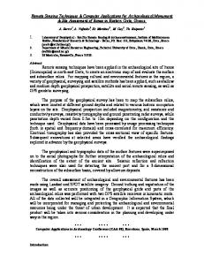
Figure Captions Figure 1. Heuristic time-series model of the relationships between sea ice physical properties and the nature of C-band microwave interactions, throughout the thermodynamic growth cycle. The lower panel shows potential geophysical information contained in microwave backscatter record. Figure 2. Summary of (a) experimental power absorption and (b) equivalent penetration depth in sea ice, at varying microwave frequencies [22]. Figm 3. Wet snow (a) permittivity (e’); (b) loss factor (E”) at volume fractions of water of 0-12%, with constant snow density of 250 kg m-3, and; (c) frequency-dependent penetration depth for varying snow water content [22]. Figure 4. Fully polarimernc microwave scattering model results from L-band simulations of thin ice in March 1988 in the Beaufort Sea [28]; (a) compares measured VV-,hh- and hv-pol. backscatter and simulated data; (b) indicates the magnitude Ipl of the complex correlation between vv and hh linearly polarized returns; (c) shows the corresponding phase of p.

18

-15” CST,F,

05

SEA :E

00

SVC

15

----

---

-----

0012

. . . . . . . . . . . . . . . . . . . . . , THICKENING

----

=-----

. . . .

. . . .

. . . .

. . . .

. , . , . . . #. , . . . . . , . , . .’.’,’ . . . . . . . . . . . . . . . . . . . . . . . . . . . . . . . . . . . . . .

E vENTS . . . . . . . . . . . . .

. .’,’.’.’ . . . . . . . . . . . . . . .

.‘,’.’..,’...’..,’,’,’,’.’,’.’,’>’,’. . . . . . . . . . . . . . . . . . . . . . . . . . . . . . . . . . . . . . . . . . . . . . . . . . . . . . . . . . .

_- ---

-- 1

--- --

.-

. . . . .

. . . . .

. . . . .

# . , , ,’ . . . . . . ?’..,’ . . . ,’.’,’.’ . . . . ,’.’, . . ..,.,., . . . . . . . . . . . . . . . . . . . . . . . . . .. . . . . . . . . . . . . . . . . . . .

. . . . .

. . . . .

_- .-

. ...’.’ .’/’? . . .’.’... . . ,,, . . .,,.,. . . . . . . . . . . . . . . . . . . . . . . . . . . . . . . . . . . . . . . . . . . . . . . . . . . . . , , / , / , , . . . . . . . . . . . . . . . . . . ./,,,.,.,., . . . . . . . . . . . . . . . . . . . . . . . . . . . . . . . . . . . . . . . . . . . . . . . . . . . . . . . . . . . . . . . . . . . . . . . . . . . . . . . .

FLLJWNG

-.

Oam 0002 PI

012

-

00s

-

0C8

-

002

-

. ,.,. . . . . .,.,. ...’.’.., . . ,... . . . . . . . . . . . . . . . . . . . . . . . . . . . . . . . . . . . . . . . . . . . . . . . . . . . . . . . . . . . , . ..,?...,?, . . . . . . . . . . . . . . . . . . . . . . . . . . . . . . . . . . . . . . . . . . . . . . . . .

SR!NE WICKING SALWE SNOW

. ,,,. . . . . . . . . . . . . . . . . . . . . . . . .

. .,,. ,,,. . . . . . . . . . . . . . . . . . . . . . . . . . . . . . . . . . . . .

. ,,. ,... ..?.? . . . . .../,. . ..... .. . . . . . . . . . . . . . . . . . . . . . . . . . . . . . . . . . . . . . . . . . . . . . . . . . . . . . . . . . . . . . . . . . . . . . . . . . . . .,. . ..,,.,,., . . . . . . . . . . . . . . . . . . . . . . . . . . . . . . . . . . . . . . . . . . . . \ . . . . . . . . . . . . . . . .. . . . . . . . .

.,,. ,,,.. . ,,. ,.,.. ,, ,,,. .,,.

COMPLETE MELT

. . ,,,. . . ,.. . . . . . . . . ,//,. . . , . . ,,. . .,., . . . . . . . . . . . . . . . . ./,,. . . . . . . . ,,,. . . , ..cE . /,,,,/./ . . . . . . . . ,,,. . . . . ,,,. . . ,,/, . . . , . . ,,. . .

-------

-----

01 WOW .VETNESS 3Y VOLUME

. . . .

GRAWTATIONM BRINE C+TAINAGE

OLWS

T~r2WC

s Talrswc PONO!NG

. . . . . . . . . . . . . . . . . . . . . . . . . . . . . . . . . . . . . . . . . . . . . . . . . . . . . . . . . . . . . . , , , -------:--------------------

SUMMER

SPRING -19C

-

‘HICKNESS

jULi( ?/EAN ‘:E SALINITY

WINTER

FALL

to

I

.— —_-

--__

----—

-

-

RESIOUAL

-

-

-

YEAFF ICE ---

-

----

EVENTS OURING WARM PERIODS

\

\

I

No SNow WETNESS I NEGATIvE UNLESS FL~

FREEZE ? lltAW EVENTS

FREEWARO

FUNICUIAR ----—---——PENDuLAR

REGIME

-—---

PONOWG ---

CATASTROPNFC ORAINAGE

{

REGIME

I

0

10

‘ FROST FLOWER

~ELATIvE SN~

:; ;

SURFACE SCATTERING SUFFICIENCY

II 8*