and mining large amounts of data from heterogeneous sources over an ... Data warehouses and OLAP systems help to analyze complex multidimensional.
OLAP Formulations for Supporting Complex Spatial Objects in Data Warehouses Ganesh Viswanathan & Markus Schneider Department of Computer & Information Science & Engineering University of Florida Gainesville, FL 32611, USA {gv1, mschneid}@cise.ufl.edu
Abstract. In recent years, there has been a large increase in the amount of spatial data obtained from remote sensing, GPS receivers, communication terminals and other domains. Data warehouses help in modeling and mining large amounts of data from heterogeneous sources over an extended period of time. However incorporating spatial data into data warehouses leads to several challenges in data modeling, management and the mining of spatial information. New multidimensional data types for spatial application objects require new OLAP formulations to support query and analysis operations on them. In this paper, we introduce a set of constructs called C 3 for defining data cubes. These include categorization, containment and cubing operations, which present a fundamentally new, user-centric strategy for the conceptual modeling of data cubes. We also present a novel region-hierarchy concept that builds spatially ordered sets of polygon objects and employs them as first class citizens in the data cube. Further, new OLAP constructs to help define, manipulate, query and analyze spatial data have also been presented. Overall, the aim of this paper is to leverage support for spatial data in OLAP cubes and pave the way for the development of a user-centric SOLAP system. Keywords: spatial data cube, user-centric OLAP, region hierarchy
1
Introduction
Data warehouses and OLAP systems help to analyze complex multidimensional data and provide decision support. With the availability of large amounts of spatial data in recent years, several new models have been proposed to enable the integration of spatial data in data warehouses and to help analyze such data. This is often achieved by a combination of GIS and spatial analysis tools with OLAP and database systems, with the primary goal of supporting spatial analysis dimensions, spatial measures and spatial aggregation operations. However, this poses several new challenges related to spatial data modeling in a multidimensional context, such as the need for new spatial aggregation operations and ensuring consistent and valid results. Moreover, existing commercial geographic
data management systems force database designers to use logical data structures heavily influenced by implementation concerns. This paper takes an unique approach to alter this implementation dependent view for modeling OLAP systems, by using a lattice theoretic approach based on the (hyper)cube metaphor to model multidimensional data. We present a user-centric conceptual modeling strategy that incorporates spatial data as first class citizens in data hierarchies. The modeling and querying of complex hierarchical structured multidimensional data in a large scale presents interesting challenges through the entire spectrum of spatial data warehouse development from designing conceptual data models accommodating complex aggregations on hierarchical, multidimensional spatial data, to developing the logical schema and finally, storage and the physical implementation. In this paper, we focus on the conceptual data model design that would allow the user to easily yet effectively create spatial data cubes, and navigate and analyze them. The model we present here is an extension of the BigCube approach [1] that presents a strict type structured hierarchy of classes to model the hierarchical data dimensions in data cubes. We start by introducing a new region-hierarchy or regH representation for complex structured region objects into a partially ordered lattice structure. Then, we introduce the C 3 constructs, which stand for the three primary constructs required for data-cube creation and maintenance, namely, Categorization, Containment and Cubing or Combination. Categorization helps to organize base data values into meaningful categories, containment helps to assign a hierarchy of ordering over the categories, and finally cubing forms an association between categories of different hierarchies in order to signify a new subject of analysis (measure value). Further, we also introduce new OLAP formulations to support the spatial data in cubes, such as the geo construct operator which allows the creation of new spatial regions from complex region hierarchies to facilitate analysis. The rest of this paper is organized as follows. Section 2 reviews existing work in spatial data warehousing and provides a case study in the form of a Product Sales data cube that is used in the rest of the paper. Section 3 presents the regH concept, which is a region-hierarchy specification to help incorporate complex structured spatial objects in data warehouses for performing analysis. Section 4 presents the C 3 constructs for spatial data cube definition and construction. Section 5 presents new OLAP formulations such as geo construct, slice and dice, and discusses spatial topological relations among complex regions using the poset structures. Finally, Section 6 concludes the paper and mentions topics for further research.
2
Related Work
Spatial data warehousing (SDW) has become a topic of growing interest in recent years. This is primarily due to the explosion in the amount of spatial information available from various sources such as GPS receivers, communication media, online social networks and other geo-spatial applications. Consequently several spatial OLAP tools are now available to help model and analyze such data.
An early approach to spatial online analytical processing (SOLAP) is [2], which mentions essential SOLAP features classified into three areas of requirements. The first is to enable data visualization via cartographic (maps) and non-cartographic displays (e.g., 2D tables), numeric data representation and the visualization of context data. Second, data exploration requires multidimensional navigation on both cartographic and non-cartographic displays, filtering on data dimensions (members) and support for calculated measures. The third area discussed involves the structure of the data, for example, the support for spatial and mixed data dimensions, support for storage of geometric data over an extended time period, etc. The conceptual design models for spatial data warehouses are extensions of ER and UML diagrams or ad-hoc design approaches. Among extensions of ER models, [3] presents a clear integration of spatial data for OLAP by extending the MultiDimER and MADS approaches. Among other ad-hoc design approaches, [4] presents a formal framework to integrate spatial and multidimensional databases by using a full containment relationship between the hierarchy levels. In [5], the formal model from [6] is extended to support spatially overlapping hierarchies by exploiting the partial containment relations among data levels, thus leading to a more flexible modeling strategy. For a comprehensive review of spatial data warehouse design models the reader is referred to [7, 8]. For modeling spatial data there are now several established approaches in the database community. [9, 10] provide a robust discussion of spatial data types by introducing types such as point, line and region for simple and complex spatial objects and describe the associated spatial algebra. Composite spatial objects (collections of points, lines and regions) are presented as spatial partitions or map objects. Similarly, the Open GIS Consortium also provides a Reference Model [11] as a standard for a representing geo-spatial information. Qualitative spatial operations include topological relations [12] such as disjoint, meet, overlap, equal, inside, contains, covers and coveredBy, and cardinal direction relations. Quantitative relations on spatial objects include metric operations based on the size, shape and metric distances between objects or their components. All these operations can be used to query and analyze spatial data in the data warehouse.
3
Modeling Data Cubes With Complex Spatial Data
In this section, we describe a new approach to design and model cubes for complex, hierarchical, multi-structured data. Spatial data such as points, lines and polygons or regions often display such semantics. Consider for example, Figure 1 that illustrates a complex region object which consists of three regions with one of them inside the hole of another. The figure also displays a single face of a region object (which can also be regarded as a simple region) with multiple holes. To facilitate the handling of such complex data in multidimensional data cubes, we introduce the regH or region-hierarchy concept that aims to provide a clear hierarchical representation of a complex region that can be incorporated as first class citizens into spatial data cubes.
exterior
interior
boundary
(a)
(b
Fig. 1. Illustration of (a) a complex region object with three faces and its interior, boundary and exterior point sets, and (b) a single face, also denoted as a simple region with holes.
The first step to accommodate complex spatial data in OLAP cubes is to explore and extract the common properties of all structured objects. Unsurprisingly, the hierarchy of a structured object can always be represented as a directed acyclic graph (DAG) or more strictly, as a tree. Figure 2a provides a more detailed visualization of a complex region object with three faces labeled as F1, F2 and F3. The interior, exterior and boundary point sets of the region are also displayed. After performing a plain-sweep operation the cyclic order of the region’s boundary is stored to represent a each face uniquely. Figure 2b shows such as tree structure of a region object. In the figure, face[ ], holeCycle[ ], and segment [ ] represent a list of faces, a list of hole cycles and a list of segments respectively. In the tree representation, the root node represents the structured object itself, and each child node represents a component named sub-object. A sub-object can further have a structure, which is represented in a sub-tree rooted with that sub-object node. For example, the region object in Figure 2a consists of a label component and a list of face components. Each face in the face list is also a structured object that contains a face label, an outer cycle, and a list of hole cycles, where both the outer cycle and the hole cycles are formed by segments lists. Further, we observe that two types of sub-objects can be distinguished called structured objects (SO) and base objects (BO) [13]. Structured objects consist of sub-objects, and base objects are the smallest units that have no further inner structure. In a tree representation, each leaf node is a base object while internal nodes represent structured objects. A tree representation is a useful tool to describe hierarchical information at a conceptual level. However, to give a more precise description and to make it understandable to computers, a formal specification would be more appropriate. Therefore, we propose a generic region-hierarchy as an alternative of the tree representation for describing the hierarchical structure of region (or multi-polygon) objects. Thus, we can define the structure of a region object from Figure 2b with the following structure expression: hregion : SOi := hregionLabel : BOihf ace : SOi[ ]. In the expression, the left side of := gives the tag declaration of a region object and the right side of := gives the tag declarations of its components, in this case, the
F3 C4
F2 C3 C2 C1
F1
(a)
(b)
Fig. 2. Illustration of a complex structured region showing faces F1 (containing cycles C1 and C2), F2 (cycle C3) and F3 (cycle C4), and a hierarchical representation for the region (or multi-polygon) object.
region label and the face list. Thus, we say the region object is defined by this structure expression. Using this representation, we can now recursively define the structure of structured sub-objects until no structured sub-objects are left undefined. A algebraic list of structure expressions then forms a specification. We call such a region specification that consists of structure expressions and is organized following some rules a region-hierarchy or regH. It can be observed that the conversion from a tree representation to the regH is simple. The root node in a tree maps to the first structure expression in the region-hierarchy. Since all internal nodes are structured sub-objects and leaf nodes are base sub-objects, each internal node has exactly one corresponding expression in the regH, and leaf nodes require no structure expressions. The regH for a region object corresponding to the tree structure as in Figure 2a is thus defined as follows: hregion : SOi := hregionLabel : BOihf ace : SOi[ ]; hf ace : SOi := hf aceLabel : BOihouterCycle : SOihholeCycle : SOi[ ]; houterCycle : SOi := hsegment : BOi[ ]; hholeCycle : SOi := hsegment : BOi[ ]; The region-hierarchy provides a unique representation for complex multistructured regions. This can be incorporated into data hierarchies in OLAP cubes by using the extract and union operators specified in section 5.
4
Data Model and C 3 constructs
In this section, we present our data model for multidimensional data cubes supporting complex hierarchical spatial objects. These are extensions to the BigCube approach [1], which is a conceptual metamodel for OLAP data defined over several levels of multidimensional data types. To support complex objects in data warehouses we need new constructs that can handle data with complicated structures. However to keep the data warehouse modeling user-friendly, the approach taken for conceptual modeling and for applying aggregations must be simple. The C 3 constructs presented here satisfy both these requirements by providing the analyst with three simple and
logical operations to construct data cubes, namely categorization, containment and cubing. Later by using classical OLAP operations such as slice, dice, rollup, drilldown and pivot, users can navigate and query the data cubes. Categorization helps to create groupings of base data values based on their logical and physical relationships. Containment helps to organize the data categories into levels and place them in atleast a partial ordering in order to construct hierarchies. Cubing or Combination takes different categories of data from the various hierarchies an helps to create a data cube from them by specifying meaningful semantics. This is done by associating a set of members defining the cube to a set of measures placed inside the cube. Further, each of the C 3 constructs have a set of analysis functions associated with them, called the A-set . An A-set can include aggregation functions, query functions such as selections, and userdefined functions (UDFs). Since aggregations are fundamental to OLAP cubes, we first introduce the definition of an A-set in Definition 1. Definition 1. Analysis set or A-set . An analysis set or A-set is a set of functions defined on the components of a data cube that are available for aggregation, querying and other user-defined operations. An A-set has the following algebraic structure: A =< {a1 , ..., an }, {q1, ..., qn }, {u1, ..., un} > where, ai represents the ith aggregation function available, qi the ith query function available and ui the ith user-defined function (UDF) available in that particular cube component. The A-set is available as part of every category, hierarchy, perspective (data dimension) and subject of analysis (fact) in the data cube. The operations on the constituent elements of these cube components are specified by its corresponding A-set . Next, to facilitate the development of the C 3 constructs and additional OLAP formulations, we present some necessary terminology and definitions based on lattice theory [14] and OLAP formalisms [15, 1]. Definition 2. Poset and its Top and Bottom Elements A partially ordered set or poset P is a set with an associated binary relation � that for any x, y and z, satisfies the following conditions: Ref lexivity : x≤x T ransitivity : ∀x ≤ y and y ≤ z ⇒ x ≤ z Anti-Symmetry : ∀x ≤ y and y ≤ x ⇒ x = y For any S ⊆ P, m ∈ P is a maximum or greatest element of S if ∀x ∈ S : (m ≥ x), and is represented as maxP. The minimum or least element of P is defined dually and represented as minP. A poset (P, �) is a totally or linearly ordered set (also called chain) if ∀x, y ∈ P ⇒ x ≤ yory ≤ x With an induced order, any subset of a chain is also a chain.
y
TIME (Year) Year: ms_date Sales Quantity : ms_int Profit : ms_int
Month : ms_date Day : ms_date
Country : ms_string
Name : ms_string PRODUCT (Name) x
Zone : ms_region
y
... 2007 2008 TIME (Year) 2009 2010
Subjects: Sales Qnty. = 10 units Profit = 1500 USD
State : ms_string County : ms_string City: ms_string LOCATION (Country)
(a)
iPhone PRODUCT (Name) Rubix cube USA Italy ...
x
LOCATION (Country)
(b)
Fig. 3. Product-Sales BigCube (a) structure shows three perspectives: Time, Product and Location that define two subjects of interest: Sales-Quantity and Sales-Profit, and a (b) sample instance.
The greatest element of P is called the top element of P and is represented as ⊤, and its dual, the least element of P is called the bottom element of P and represented as ⊥. A non-empty finite set P always has a ⊤ element (by Zorn’s Lemma). OLAP cubes often contain sparse data. To ensure that a bottom element exists and to make the OLAP operations generically applicable to all multidimensional cube elements, we perform a lifting procedure where given a poset P (with or without ⊥), take an element 0 ∈ / P and define � on P⊥ = P ∪ {0} as: x ≤ y iff x = 0 or x ≤ y in P. Definition 3. Lattice Let P be a poset and let S ⊆ P. An element u ∈ P called an upper bound of S if ∀s ∈ S : (s ≤ u). Dually, an element l in P is called the lower bound of S if ∀s ∈ S : (s ≥ l). The set of all upper bounds and lower bounds is represented as S u and S l respectively. S u = {u ∈ P | (∀s ∈ S) : s ≤ u} S l = {l ∈ P | (∀s ∈ S) : s ≥ l} An element x is called the supremum or the least upper bound of S if: x ∈ S u and ∀x, y ∈ S u : x ≤ y. This is represented as supS or ∨S. The infimum or the greatest lower bound of S is defined dually and represented as inf S or ∧S. A non-empty ordered set P is called a lattice if ∀x, y ∈ P : x ∨ y and x ∧ y. Example: Consider the classical product-sales multidimensional dataset as shown in Figure 3a. The data cube has product, location and time perspectives (or data dimensions), and sales quantity and profit, for example, as the subjects of analysis (or facts). There are several hierarchies on location perspective such as {city,county,zone,country} and {city,state,country}. An instance of the data cube is shown in Figure 3b.
The basic data that needs to be stored (and later analyzed) in the data warehouse are values such as 1500 (of type int ) for the profit in USD and “Gainesville” (of type string) for the City name. These are called the base data values of the dataset. The base data type for each value is indicated within parenthesis. According to their functionality, base data values can be either members when used for analysis along data dimensions, or measures when used to quantify factual data. Now we introduce the C 3 constructs and supporting OLAP formulations. Real-world data always has some form of symmetric and asymmetric nature associated with its base data values. For e.g., all persons working in a University can be employees (symmetric relationship). Employees could be students, faculty or administrators (asymmetric relationship). Definition 4. The first C in C 3 : Categorization. A categorization construct defines groupings of base data values based on the similarity of data as: hC, Ac i where C is a category (collection of base values) and A is a set of analysis functions that can be applied on the elements of C. The base data values can be members or measures of the data warehouse. The exact semantics of categorization relationships are defined in one of three ways: arbitrary (for e.g., split 100 base values into 10 categories equally according to some criteria), user-defined (for e.g., Gainesville, Chapel Hill and Madison can be categorized as College Towns), or according to real-world behavior (such as spatial grouping, for e.g., New Delhi, Berlin and Miami can be categorized as Cities). Examples of A-set functions on such categories include string concatenation, grouping (nesting) and the multiset constructor. Example: In our case study, two examples of categories are City={(“Gainesville”, “Orlando”, “Miami”)} and Profit={ (“1500, “10000, “45000”)} for the profit in USD. These are of types string and int respectively. Definition 5. Category, Category Type and CATEGORY. A category of elements c ∈ S, S ⊆ BASE, is a grouping of base data values such that a valid categorization relationship exists among the set of elements. A category type, provides the multiset data types for each category. The set of all available category types is defined as a kind CATEGORY. Categories help us to construct higher levels of BigCube types, namely hierarchy, perspective and subject. Hierarchies are constructed using the containment construct over the categories, and perspectives are defined as a combination of hierarchies. Definition 6. The second C in C 3 : Containment. The Containment construct helps to define hierarchies in the data. These data hierarchies are modeled as partially ordered sets (or posets) to use an extensible paradigm that supports different kinds of ragged and unbalanced hierarchies. The containment construct
takes one or more data categories and builds a new partial ordering (data hierarchy) from it. These data hierarchies are part of the generalized lattice structure that is established by the partial ordering of the constituent categories. The containment construct is defined as a set inclusion from one level to another as < P, Q, �, A >, where P and Q represent the categories of data on which � holds. The containment construct is analogous to a single path between two levels in a poset. The set of analysis functions that are applicable on a particular containment are available in A. These functions can be applied which moving from the elements of one category to another. This helps to uniquely define operations on specific hierarchical paths in the perspectives of the cube. The semantics of the containment construct is defined by: (i) any arbitrary containment, for e.g., fifteen base data values can be ordered into a four- level hierarchy using the structure of a balanced binary tree, (ii) user-defined containment : for e.g., products can be ordered into a hierarchy based on their selling price, (iii) according to real-world behavior: these reflect the fact that a higher level element is a context of the elements of the lower level, it offers constraint to the lower level values, it evolves at a lower frequency than the lower level elements, or that it contains the lower level elements. To define the multidimensional cube space we now need to third C in C 3 which is the cubing or combination construct. Before arriving at this, we first need to define the direct product of two lattices. Definition 7. Direct Product. The direct product P × Q of two posets P and Q is the set of all pairs (x, y), x ∈ P and yinQ such that (x1 , y1 ) ≤ (x2 , y2 ), iff x1 ≤ x2 in P and y1 ≤ y2 in Q. The direct product generates new ordered sets from existing posets. The direct product L1 × L2 of two lattices L1 and L2 is a lattice with ⊤ := (x1 , y1 ) ∧ (x2 , y2 ) = (x1 ∧ x2 , y1 ∧ y2 ) and ⊥ := (x1 , y1 ) ∨ (x2 , y2 ) = (x1 ∨ x2 , y1 ∨ y2 ) for all x1 , y1 ∈ L1 , x2 , y2 ∈ L2 and (x1 , y1 ), (x2 , y2 ) ∈ L1 ×L2 . The use of direct product enables the creation of perspectives and subjects of analysis from a combination of member and measure value lattices. Definition 8. The third C in C 3 : Cubing or Combination. The Combination construct helps to map two semantically unique categories of data values by a set of analysis functions. Given two ordered sets of categories P and Q, we define a order-preserving (monotone) mapping ϕ : P → Q such that if x ≤ y in P ⇒ ϕ(x) ≤ ϕ(y) in Q. Now, the combination construct is defined as hP, Q, ϕ, Ai, where A is the set of analysis functions that can be applied on the combination relationship. A collection of lattices are together taken as perspectives combine to determine the cells of the BigCube, each containing one or more subjects of analysis. Semantically, subjects of analysis are thus unique, in that they are functionally determined by a set of perspectives, however, they are structurally similar to perspectives in being a collection of lattices.
Definition 9. BigCube. Given a multidimensional dataset, the BigCube cell structure is defined as an injective function from the n-dimensional space defined by the Cartesian product of n functionally independent perspectives P (identified by its members) to a set of r subjects (identified by its measures) S and quantifying the data for analysis as: fB : (P1 ⊗ P2 ⊗ . . . ⊗ Pn ) −→ Si where i ∈ {1, . . . r} ∧ (Si , P ) ∈ BASE The complete BigCube structure is now defined as a union of all its cells, given as: [ Si BigCube (B) = i∈{1,...r}, fB
5
Spatial OLAP formulations with the C 3 Constructs
In this section, we present OLAP formulations that help to apply analysis operations on data cubes with complex spatial data by using the C 3 constructs on the BigCube model. First, we analyze how data cubes can be easily designed and modeled using the C 3 constructs as follows. The basic, low-level data types are available in the kind BASE. These include alphanumeric, time and geo-spatial data types. Elements of these types are the base data values which are first organized into Categories by using the categorization construct. This means that for e.g., “GNV”, “LA”, “MN” can be a category of cities. Analysis functions can be associated to the domain of the categories. For e.g., we can define a union function that takes the elements of cities and performs a union operation to yield a new polygon (country). The geo construct operation allows to extract any face of the complex region from the regH and construct a new region from it, for example, a city (Gainesville) from the country (USA). This is done using three topological operations interior, boundary and closure that remove possible anomalies such as dangling points or lines in the structure of the region. The interior A◦ of a region A is given by the set of points contained inside the region object. The boundary ∂A gives the set of points covering the object. Thus, A◦ ∪ ∂A gives the closure A of A and this is used to construct the regH for the new spatial object from the base segment lists. The next step is to use the containment construct to define the hierarchical nature of the elements within the categories. This allows for the creation of explicit hierarchical paths between categories and the specification of analysis operations on each of them on uniquely or as a whole. An e.g., of analysis being using the containment construct is the often-used SUM aggregation operator on Sales quantity defined from City to State level. The final step is the creation of interacting lattice galaxies which is achieved by using the combination construct. The combination construct maps the categories in different hierarchies to others in the galaxy to create the data cube
schema (cells). Elements of the data cube (objects within the cells) are identified by their defining cube perspectives. We now provide examples of OLAP formulations that can applied on the BigCube types and their instances thus defined. Consider a BigCube Bwith n perspectives and i subjects of analysis. Let m1 , . . . , mn be members from each of the n perspectives defining the set of measures b1 , . . . , bi . Then, the restrict operator returns the cell value by following the cubing from upto n perspectives of the BigCube as hhm1 , . . . , mn i, b1 , . . . , bi i. For example, the sales quantity of iphones in Gainesville region in March 2011 is given by hh“iPhone”, “Gainesville”, “March2011”i, 50i. The slice operation removes one perspective and returns the resulting BigCube and dice performs slice across two or more perspectives. The resulting cells have the structure hhm1 , . . . , mk i, b1 , . . . , bi , Ai, where 1 ≤ k ≤ n and A provides the set of aggregation functions applicable on the measures of this subcube. These operations change the state of the BigCube, because any change in perspectives redefines the cells (measures) in it. Pivot rotates the perspectives for analysis across axes and returns a BigCube with a different ordering of subjects. Roll-up performs specialization transformation over one or more constituent hierarchical levels, and drill-down applies the generalization transformation over one or more hierarchical levels. Given members m1 j, . . . , mk j, 1 ≤ j ≤ n denoting k levels of ordering in each of the n perspectives, roll-up and drill-down operations yield a different aggregated state of the cube, as, hhm1 j, . . . , mk ji, s1 , . . . , si , Ai i, where si = fi (b1 , . . . , bi ), f ∈ A. Drill-through obtains the base data values with highest granularity. Drill-across combines several BigCubes in order to obtain aggregated data across the common perspectives. For spatial measures, spatial relationships can be given directly by checking with the C 3 constructs and ordering in the poset. For example, to check for containment of a region X in region Y, we check the containment construct on X and Y. If hX, Y, �, Ai exists with X � Y , then X is contained in Y. Similarly, the largest area contained contained in one or more given areas Xi is given by ⊥X . Dually, the smallest area containing one or more given areas Yj is given by ⊤Y . In this manner, lattice ordering along with the categorization, containment and cubing constructs provide a minimal set of formulations to create, manipulate and query spatial data cubes in a user-friendly manner.
6
Conclusions and Future Work
In this paper, we present a novel modeling strategy to incorporate support for complex spatial data in OLAP data cubes. First, we introduce a region-hierarchy that helps to represent a complex region object (with several faces and multiple holes) in a uniquely distinguishable manner. Then we present three new constructs called C 3 , involving categorization, containment and cubing or combination that together help to easily build data cubes in a multidimensional environment. This provides a framework consisting of a user-friendly conceptual cube model that abstracts over logical design details such as star or snowflake
schema and other implementation details. Later, new OLAP formulations are specified for manipulating spatial data hierarchies (geo construct ), and for querying. Overall, this region-hierarchy provides a unique approach to include spatial regions as first class citizens of data hierarchies in multidimensional data cubes. In the future, we plan to provide the complete set of OLAP operations for manipulating and querying spatial data cubes, and to provide translations from the hypercube to logical design (relational and multidimensional) to facilitate implementation of the SOLAP system.
References 1. Viswanathan, G., Schneider, M.: BigCube: A MetaModel for Managing Multidimensional Data. In: Proceedings of the 19th Int. Conf. on Software Engineering and Data Engineering (SEDE). (2010) 237–242 2. Rivest, S., Bedard, Y., Marchand, P.: Toward Better Support for Spatial Decision Making: Defining the Characteristics of Spatial On-line Analytical Processing (SOLAP). Geomatica-Ottawa 55(4) (2001) 539–555 3. Malinowski, E., Zim´ anyi, E.: Representing Spatiality in a Conceptual Multidimensional Model. In: 12th ACM Int. workshop on Geographic Information Systems, ACM (2004) 12–22 4. Ferri, F., Pourabbas, E., Rafanelli, M., Ricci, F.: Extending Geographic Databases for a Query Language to Support Queries Involving Statistical Data. In: Int. Conf. on Scientific and Statistical Database Management, IEEE (2002) 220–230 5. Jensen, C., Kligys, A., Pedersen, T., Timko, I.: Multidimensional Data Modeling for Location-based Services. The VLDB Journal) 13(1) (2004) 1–21 6. Pedersen, T., Jensen, C., Dyreson, C.: A Foundation for Capturing and Querying Complex Multidimensional Data. Information Systems 26(5) (2001) 383–423 7. Viswanathan, G., Schneider, M.: On the Requirements for User-Centric Spatial Data Warehousing and SOLAP. Database Systems for Advanced Applications (2011) 144–155 8. Malinowski, E., Zim´ anyi, E.: Advanced Data Warehouse Design: From Conventional to Spatial and Temporal Applications. Springer-Verlag (2008) 9. Shekhar, S., Chawla, S.: Spatial Databases: A Tour. Prentice Hall (2003) 10. Guting, R., Schneider, M.: Realm-based Spatial Data Types: The ROSE algebra. The VLDB Journal 4(2) (1995) 243–286 11. Open GIS Consortium: Reference Model: (Accessed: April 11, 2010) http://openlayers.org. 12. Schneider, M., Behr, T.: Topological Relationships between Complex Spatial Objects. ACM Transactions on Database Systems (TODS) 31(1) (2006) 39–81 13. Chen, T., Khan, A., Schneider, M., Viswanathan, G.: iBLOB: Complex Object Management in Databases through Intelligent Binary Large Objects. 3rd Int. Conf. on Objects and Databases (2010) 85–99 14. Davey, B., Priestley, H.: Introduction to Lattices and Order. Cambridge University Press (2002) 15. Gray, J., Chaudhuri, S., Bosworth, A., Layman, A., Reichart, D., Venkatrao, M., Pellow, F., Pirahesh, H.: Data cube: A Relational Aggregation Operator Generalizing Group-by, Cross-tab, and Sub-totals. Data Mining and Knowledge Discovery 1(1) (1997) 29–53