Nevertheless, our experience in the solution of solid and structural mechanics problems as weil as observations from the corresponding examples in the cited ...
~
Computers & Structures
PERGAMON
Computers and Structures 80 (2002) 1523-1536 www.elsevier.com/locate/compstruc
On applications of parallel solution techniques for highly nonlinear problems involving static and dynamic buckling Th. Rottner a
a,
K. Schweizerhof a,*, 1. Lenhardt
b, G. Alefeld b
InstituteJor Mechanics,UniversityoJ Karlsruhe,Kaiserstr.12, 76128Karlsruhe,Germany
b Institute Jar Applied Mathematics, University oJ Karlsruhe, Kaiserstr. 12, 76128 Karlsruhe, Germany Received 10 January 2001; accepted 4 May 2002
Abstract Within this contribution the efficient finite element analysis of shell structures with highly nonlinear behavior is presented. The coupled nonlinear system of equations resulting from the FE discretization is solved using Newton-like procedures, thus the solution of a linear system of equations is needed in each Newton iteration. For fine discretizations the resulting linear systems of equations become very large and their solution dominates the computational effort. Consequently, parallel computers offer major capabilities to reduce the CPU time needed. A geometrical approach for parallelization is used, standard methods for the graph partitioning are employed. It is weil known that iterative methods for the solution of linear equation systems are much more suitable for parallelizing compared to direct methods. Therefore in a first step the use of such methods is investigated for the application to badly conditioned problems typical for shell problems in particular in failure situations with alm ost singular matrices. In the analysis of shell structures with tendencies to buckle a static and a dynamic approach are discussed considering both physical and computational aspects. @ 2002 Elsevier Science Ltd. All rights reserved.
1. Introduction For stability investigations of structures in solid mechanics usually a static approach is preferred in combination with a finite element discretization. Such a procedure involves the computation of so-called stability points and mostly path-following algorithrns are needed to judge the postbuckling behavior. In addition eigenvalue analyses are often performed. Such approaches are very successful for medium size models with fairly small numbers of degrees of freedom. However, for more complex structures as e.g. silo shells such a method does not lead to a: reliable estimate of the real postbuckling behavior due to the many solution paths possible. In addition, within a Newton-Raphson solution convergence becomes a problem as the matrices become
.Corresponding
author.
singular resp. almost singular in a large part of the postbuckling regime. Thus, it seems to be advisable to investigate the real problem including the time dependency of the buckling process performing a nonlinear transient analysis. Both types of analysis require a fine discretization as local effects are important also for the global response and the models contain large numbers of unknowns. Parallelization of the complete solution process is a must and has been carried out for static nonlinear analyses even with rather badly conditioned system matrices. The latter is-aside from the singularities due to the structural behavior-a result of the discretization with shell elements in general. In transient analyses the conditioning of the matrices ameliorates compared to static analyses, thus iterative solvers should be even better suited for the solution. Besides the adjustment of the time integration schemes for a fully parallel solution, it is also an important aspect to choose an efficient but still
0045-7949/02/$ - see front matter @ 2002 E1sevier Science Ltd. All rights reserved. PlI: S0045-7949(02)OO 107-4
1524
Th. Rottner et al. / Computers and Structures 80 (2002) 1523-1536
reliable preconditioning strategy taking advantage of the knowledge that with constant time step size the system matrix changes only fairly little in most cases. In Section 2 basic equations for the static and transient finite element analyses are given and the applied solution strategies are introduced. Direct and iterative solvers for the solution of the arising systems of linear equations and their properties are discussed in Seetion 3. For a nonlinear static problem, the efficiency of the different solvers is compared. With the restrietion to iterative solvers the parallelization is performed and some results are presented in Section 4 to show the efficiency of the approach. Finally, in Section 5 the problem of an axially loaded cylindrical silo shell is investigated. EspeciaIly the question of the modeling of the problemeither static or transient-is addressed. As the efficiency of the solution process is strongly affected by the modeling, this aspect is also investigated in more detail.
2. Governing equations and solution strategies 2.1. Static analyses In nonlinear finite element analyses nonlinear systems of equations have to be solved: G(u, Je)= Ap - r(u) = O.
(1)
Herein r is the vector of the internal farces, p is the externalload vector, },is a scalar load parameter and u are the nodal displacements. As it is weIl known, the application of Newton's method leads to an incremental iterative solution procedure, in which for every load step m linear systems of equations KT(Ui) . /),.u= r(ui) - },mp = /),.r,
i = 1,2,...
(2)
have to be solved. K T is the Hessian matrix (tangent stiffness matrix), /),.u is the incremental displacement vector, and /),.rthe vector of the residual forces. The update of the displacement vector u in each iteration i is given by Ui+l
= Ui +
/),.u.
(3)
For nonlinear finite element analyses of structures with snap-through or snap-back behavior also arc-length methods are neeessary (see e.g. [4,25,26,31)). The load parameter A is then treated as an additional variable. As a eonsequence, an additional constraint equation has to be introduced, anq after linearizing this equation, a linear, nonsymmetrie system of equations is obtained: KT vT
[
-p
1
CXJ
/),.r
[ ] [1 ], /),.l~
=
-
(4)
/),./,
where 1 defines the arc-length constraint, v comes from
the linearizationand 6;\ is thc incrementof the load
parameter. Performing bloek-Gaussian elimination, the solution of the linear system (4) can be obtained by solving the two symmetrie systems of equations /),.Ul= K~lp
and
/),.JI = -K~l /),.r,
(5)
and then /),.,1.= _I
+ VT/),.ull o::+vT/),.UI
(6)
and /),.u = /),.Ull+
/),.,1./),.ul.
(7)
Thus, the main effort to perform nonlinear finite element analyses is in the solution of linear, symmetrie systems of equations with sometimes indefinite tangent stiffness matrices, that-in case of thin sheIl structures-may be already iIl-conditioned in the purely linear case. For eomputations on serial computers, direct solvers are usually preferred over iterative ones, beeause onee the factorization of the stiffness matrix is performed, the solution of the two linear systems (5) can be obtained by two simple forward/baekward substitutions. Using iterative methods, the two systems have to be computed independently and almost no advantage can be drawn from the solution of the first system. In [20,21,28] a method is described, which reduces the computation time for the iterative solution of (4), but it does not completely overcome the disadvantage of the iterative solvers for strongly nonlinear analyses. The focus in Sections 3 and 4 is on the application of various iterative solver strategies even for ill-conditioned thin shell problems-and their use as solvers in a parallel implementation. In the nonlinear static solution process, the information on the stability in the sense of LJAPUNOV[22] of the structure can be obtained by monitoring the definiteness of the tangential stiffness matrix. Using direct methods for the solution of the arising linear systems of equations in Newton's method, a simple and efficient procedure is to monitor the determinant of the stiffness matrix: det(KT)
= det(LDLT) = det(L) det(D) det(LT) = det(D),
(8)
if an LDLT factorization is performed. It is a necessary condition for instability, that det(K T) becomes negative. If det(K T) is positive, however, the equilibrium is not necessarily stable, because there may be an even number of negative eigenvalues. Another criterion is based on the so-caIled inertia of the stiffness matrix, that is the tripie (n,z,p), where n is the number of negative, z the number ofzero and p the number of positive eigenvalues. Again using a LDLT faetarization with A being the diagonal matrix of eigenvalues and Q the matrix of eorresponding eigenveetors
1525
Th. Rattner et al. I Computers and Structures 80 (2002) 1523-1536
inert(A)
= inert(QTKTQ) = inert(QTLDLTQ) =
inert(XT DX)
(9)
= inert(D),
[11:2ßM+KT]I1U=Pn+1
-r(Ui)+M[U-
11:2ßUi] (16)
the inertia can be detennined by directly checking the diagonal matrix D. The number of negative eigenvalues is identical to the negative entries in D. These eriteria can then be used for the detennination of critical points. A very simple proeedure is to bisect these eritieal points; a more elegant proeedure to compute the critical points direct1y is described in [34,35]. If the eritical points are bifurcation points, also the branching solution paths have to be computed (see e.g. [18]). In addition, as proposed in [7], so-ealled fold lines can be computed, i.e. eritieal sub set paths in a multiparametric space.
is solved and an update of the displacements Un+Li:= Ui+l = Ui + l1u
(17)
has to be perfonned. After convergence, velocities and aceelerations ean then be detennined using Eqs. (12) and (13). It should be noted, that eompared to static analyses, where the coefficient matrix for the linear equation systems is the tangential stiffness matrix KT' an "effective stiffness matrix" K* = 11:2ßM + KT
(18)
2.2. Transient analyses Induding inertia effeets, the system of nonlinear differential equations now reads in a semi-discrete fonn as
Mü+r(u) =P
(10)
with the mass matrix M, the displaeements u, the accelerations Ü, the nonlinear internal forces rand the externaIload p. Starting with the known solution for the displacements Un,the velocities un and the accelerations ün at time tn, the solution at time tn+l= tn + I1t has to be detennined: Mün+!
+ r(Un+d = Pn+l.
(11)
Using the standard Newmark approach [11] leads to Un+l
= Un + I1tun+ I1r[G - ß)ün + ßün+d
(12)
and Ün+!= ün + I1t[(1 - y)ün + YÜn+d,
(13)
with the Newmark parameters ß and y. For ß = 0.25 and Y = 0.5 the Newmark method is known to be uneonditionally stable and the accuracy is then of order two. Introducing Eq. (12) into (11) leads to the nonlinear system 1 I1t2ßMun+J
+ r(un+d = Pn+l+ Mu
(14)
with
u = M~ß
(u" + MÜn)
+ (2~
- 1) Ün,
(15)
that can be solved for the displacements using Newton's method. Thus, in each Newton iteration i the linear systemof equations
is the consequence of the Newmark algorithm which will be diseussed further in Seetion 5. For the transient approach, no efficient stability criteria are available like in the static case. Some details concerning this topie are given in [29].
3. Iterative methods for solving linear systems of equations in structural mechanics The most time consuming step in the nonlinear process is the solution of the linear systems of equations (5) in the static case resp. (16) in the transient case. As especially Eq. (5) may become very ill-conditioned in the context of buckling and stability problems, often direct solvers are preferred over iterative ones. In this section, the application of iterative preconditioned Krylov-subspace methods to such a dass of illeonditioned problems is investigated. For a nonlinear example problem, the efficiency and robustness of these iterative methods are eompared to a fast direct sparse solver. A parallelization based on iterative solvers can only be suggested, if such iterative solvers lead to reliable solutions independent of the problem. 3.1. lntroduction oi iterative solvers As the tangential stiffness matrices in (5) resp. (16) are symmetrie, Krylov subspace methods like the conjugate gradient [10], the Lanczos method [19,23] and the symmetrie QMR method [8] are applied. More general methods for the solution of nonsymmetric eoefficient matrices as e.g. BICGSTAB or GMRES for the solution of the linear system in Eq. (4) appear to be 1ess eonvenient, as they require more numerical effort. The main difference between the three mentioned methods for symmetric coefficient matrices lies in the field of application. The conjugate gradient method is restricted
1526
Th. Rottner et al. I Computers and Structures 80 (2002) 1523-1536
b~a---Hb
to positive definite systems of equations, whereas the Lanczos and the QMR method can also be appliedfor indefinite systems. Since the convergence behavior of iterative methods depends strongly on the condition number of the coefficient matrix, preconditioning techniques are used to speed up the solution process. In particular, the following-partially well known-techniques are applied in this context:
.. .
Jacobi preconditioning (diagonal scaling), SSOR preconditioning with the Eisenstat trick [5], several techniques based on incomplete factorizations as e.g. - incomplete factorization on the sparsity pattern of the coefficient matrix MPILU, often referred to as ILU(O) in the literature, with diagonal modification to enforce positive definiteness, - a block version of MPILU, where the coefficient matrix can be filtered before computing an incomplete factorization Block-MPILU [27], - incomplete factorization allowing fill-in of the first level FLILU, often referred to as ILU(1) in the literature, - incomplete factorization with numerical dropping NDILU.
It should be noted, that aIl these preconditioning matrices are forced to be positive definite. This property has to hold for the conjugate gradient and the Lanczos method, but not for the QMR method. EspeciaIly this fact makes the QMR method very attractive for the following reason: Within the Newton scheme, sequences of linear equation systems have to be solved. In each Newton step, the changes of the tangential stiffness matrix are moderate. Therefore, it seems to be reasonable to re-use preconditioning matrices in subsequent Newton iterations. Thus, computationally "expensive" preconditioners may become attractive-particularly the complete factorization of the coefficient matrix, resulting in a hybrid direct/iterative scheme. However, as the tangential stiffness matrix may be indefinite in a nonlinear solution process, it can be used for preconditioning purposes in general only in combination with the symmetric QMR method.
I
.:::
1 Fig. 1. Flange: system.
loads at the left and right side, as can be seen in Fig. 1. The material behavior is assumed to be linear elastic with E
=
2.1 X 10⁵ N/mm2
and
v
= 0.3
(steel). It is a
badly conditioned thin sheIl-problem (the condition number is about 108), with sheIl thickness 3 mm, at the stiffeners 6 mm. The geometrical
data are a
= 200
mm,
b = 30 mm and h = 400 mm. The complete sheIl structure is discretized with 22,400 four-noded bilinear sheIl elements [9] which leads to 112,500 equations. In Fig. 2, the nonlinear load-deflection curve of the points A and Bof the flange-structure is depicted. There, a snapthrough-behavior can be seen; after reaching a maximum value, the load decreases and remains constant afterwards, whereas the displacements are still increasing. The deformed structure is depicted in Fig. 7. The socaIled snap-through phenomenon happens, when the dents at the left and right sides of the horizontal pipe are occurring (Fig. 3). Fig. 4 shows the computation time and the memory requirements of the above mentioned solvers for the solution of one linear system of equations on an IBM RS6000 workstation. For this problem, the two different fiIl reducing strategies 'md' and 'nd' behave quite similarly concerning computation time as weIl as memory requirement. This may change dramatically for other problems [27]. The preconditioned iterative solver, how8 7 6
-CI) 5 CI)
3.2. Numerical comparison using a benchmark problem These preconditioned iterative methods are compared to an efficient direct sparse solver SMP AK [6] using the nested dissection (nd) and minimum degree (md) strategy to permute the matrix in order to minimize fill-in. As a benchmark problem, the system in Fig. 1 is used. It is a cross-pipe with stiffeners at the ends, the latter is called flange in the following. The flange is fixed at the lower and the upper part and subjected tQ shear
E cu 4 cu Q. "C 3 cu .2 2
point A --0-point B -0-
.............-........
1 0 0
2
4
6
8 10 12 14 displacement [mm]
Fig. 2. Flange: load-detlection
16
curve.
18
20
1527
Th. Rottner et al. / Computers and Structures 80 (2002) 1523-1536 load 5tep 13
load 5tep 10
undeformed
Fig. 3. Flange: defonnation at various load steps (see marks in Fig. 2).
~ 0
100
computing time [5] and ~ 200
300
memory [MByte] 400
500
600
SMPAK (md) SMPAK (nd) cg (without) cg (Jacobi) cg (SSOR) cg (Block-MPILU) cg (MPILU) cg (FLlLU) cg (NDILU)
Fig. 4. Computing time and memory requirement on a IBM RS6000 for flange example (solving one linear system at a typicalload step).
ever, leads to faster solution of the given problem, with the exception of the NDILU preconditioning. Here, unavoidable index operations slow down the computation of the preconditioner. In this case, the most efficient solution is obtained for the Block-MPILU and the FLILU preconditioning, but also simple preconditioning strategies like Jacobi and SSOR lead to satisfactory solution times for the linear problem. It must be noted that the memory requirement for the iterative solvers is considerably smaller. Though the number of iterations required for the better preconditioners SSOR and of course the xl LU preconditioners are substantially smaller than for the Jacobi preconditioning, the corresponding algorithms need more computer memory. In addition the number of operations per iteration is substantially larger; as a consequence the overall effect represented by the computing time in Fig. 4 does hardly decrease for the "better" preconditioning algorithms. For the w,hole nonlinear solution, the same comparison is carried out on a NEC-SX4 computer. The following analyses give an impression on the effort needed for the computations along the full load-deformation path induding stable and unstable parts with partially very bad condition numbers. In order to allow a general judgement on the performance of the various algorithms beyond computing times also the memory required is
monitored. The Lanczos method is used for the iterative solution, because the tangential stiffness matrix gets indefinite within the nonlinear solution path. As can be seen from Fig. 5, the direct SMP AK solver leads to a faster solution ofthe problem. This is mainly due to the fact that with the use of the arc-length method two linear systems of Eq. (5) have to be solved within each nonlinear iteration and therefore the direct solver can reuse the LDL T-factorization. As a consequence, the direct solution of the second system is very fast. In contrast to this, the iterative solver cannot benefit from the solution of the first linear system when solving the second one, with the exception of the preconditioner, that has to be built only once. A method to speedup the iterative solution within the arc-length method is given in [20,21,28], where the system (4) is tackled. The computing times for the Block-MPILU, MPILU and FLILU, however are competitive to the direct solution. As in the linear case, the memory requirements are significantly lower for the iterative solver than for the direct one. A remarkable difference between the nonlinear and linear solution occurs for the NDILU preconditioner. In the nonlinear case, the index operations are performed only once. The resulting sparsity pattern is reused for all subsequent linear systems. Due to the high quality of this preconditioner, the time spent to create the sparsity
1528
Th. Rottner et al. / Computers and Structures 80 (2002) 1523-1536 ~ 0
computing time [min] and ~
250
500
750
.
.
memory [MByte] 1000
1250
SMPAK (md) ~'\i't4~~~~'.~.,,'~S;fu~~+~;*~ SM PAK (nd)~~A'_~j@jj\1j~!&\~1!\\\i~~ lanczos (Jacobi).%fu;~' .
-
,,,,"
;'"",.~if"~~'
"
.,~
.~
lanczos(SSOR) ~~;;!,(w
c: CI> .5:!
a;
c: :;;;
0.0 0.3646
Fig. 14. Load-deflection curve for cylinder AL-llOO, transient axial load, v = 0.01 mm/s; (a) total curve (b) dose-up at buckling point induding kinetic energy time history and load levels from experiment and German DIN norm.
4
5
6
Fig. 15. Cylinder AL-I100, deformation states, transient axial load, v = 0.01 mm/s, scaled by factor of 10.
netic energy after buckling is about 30% larger compared to the smaller velocity. The visually observed buckling process is similar and therefore not shown here. This, of course, changes with higher velocities. Similar results were obtained for a wide range of cylinders and imperfections [17,32]. Further aspects concerning such a variation are discussed in detail, particularly also for cylinders with uniform and nonuniform filling [17,32]. It must be noted that beyond the single transient analysis considered here the consideration of perturbations in combination with transient analysis allows a very good judgement of the sensitivity of a stable point on the load deflection path [27,29]. This also holds for other load cases. 5.4. Efficiency aspects All the results presented have been obtained using the parallel implementation of the FE-pro gram FEAP-
MeKa [33] as described in Section 4. Fig. 16 shows a typical domain decomposition of the structure for 16 processors using the spectral bisection algorithm [1]. However, as discussed in [30], for quasi-static computations of the axially loaded cylinders almost no benefit resulted from the utilization of parallel methods due to the very ill-conditioning of the structural problem in combination with iterative schemes for the solution of the arising linear systems of equations. This is particularly true, if the comparison of the computing time for the iterative parallel solution is not made to the corresponding iterative solution on one processor but to the most efficient sequential solution that is available, what in our case is the combination of the symmetrie QMR method [8] with one factorization per Newton step as a preconditioner [28]. Hence, in the static case, the user has no benefit from parallel processing, until other solution strategies like e.g. parallel direct methods or multilcycl mcthQds are available.
~ -.--.-
1534
Th. Rottner et al. I Computers and Structures 80 (2002) 1523-1536 100
'
d..- .., ideal ~
---
-~CG-MPILU .~~
Co ~ '0 GI GI Co UI
10
...~ .~~~_..~~~
...~_.~ . ~ ~~~ ~-~
~
~_..
~.
---~~.~---
1 2
1
For the transient analysis the situation is different. As mentioned in Seetion 2.2, for transient analyses using the Newmark method (or related methods) the tangential stiffness, whieh is rather ill-eonditioned, is not the eoeffieient matrix of the linear system of equations to be solved, but the effeetive stiffness matrix (see Eq. (18)). A doser look reveals, that deereasing the time step ßt leads to a domination of the mass term in the final matrix. As a eonsequenee, the eondition of the effeetive stiffness matrix K* ameliorates, beeause the mass matrix is symmetrie and positive definite. In Fig. 17 the solution of one linear system cf equations with the eoeffieient matrix K* at the beginning of the analysis with different values for ßt is eompared using the preeonditioned egmethod. For preeonditioning the weIl known ineomplete faetorization MPILU is applied. A signifieant saving of iterations and therefore a deereasing eomputation time ean be observed for smaIl time steps. Though it is not advisable to deerease the time step unneeessarily-as a result many more linear systems of equations would have to be solved for the simulation of the same time interval-it ean be stated, that if it is neeessary to use small time steps, one will benefit from the better eonditioning of the effeetive stiffness matrix. In Fig. 18 the speedup of the eomplete transient eomputation from Seetion 5.3.1 due to parallelization is
4
8 # processors
16
32
64
Fig. 18. Speedup of parallel solution for transient analysis compared to two different sequentia1 solutions, CG-MPILU and SQMR-LU.
given. The parallel eomputation is performed using the preeonditioned eg-method, where on the loeal domains of proeessors some ineomplete faetorizations for the preeonditionings are done (see e.g. [28]). These eomputation times are eompared to the eorresponding sequential solution (MPILU) and also to the most effieient solution proeedure available, that is the symmetrie QMR method with some eomplete faetorizations (LU), as mentioned above. The speedup is suffieiently good, if the size of the given problem is taken into account; for the eomputation with 64 proeessors eaeh domain eonsists of about 150 elements, and the proeessors are by far not loaded enough. However, it is obvious that in the transient analysis the user benefits from the parallel proeessing even eompared to the best available sequential method. Comparing the effort required for a statie vs. a transient solution there is little differenee within a solution step beyond the faet that the added mass matrix improves the eondition number of the system matrix also strongly dependent on the size of the time step. However, the physieal nature of the problem is eonsiderably different in a transient proeess, as inertial forees
250
400
200
'Z
~ 300
QJ .f->
~
;.: 200 0
QJ
E
% 100
'Z
150 100 50
0
0 u
ßt=
~
~
~
Fig. 16. Domain decomposition for 16 processors using spectra1 bisection.
~ 0
~
SQMR-LU
~~._.~~ ~~~._~.~. -~-~
- ~..
'Z cu .f-> \I)
~ 0 T"""i
~ T"""i
~ r-I
I 0 T"""i
~ N
I 0 T"""i
~ Cf:)
I 0 T"""i
~ "