On-axis joint transform correlation based on a four-level power spectrum Ignasi Labastida, Arturo Carnicer, Estela Martı´n-Badosa, Ignacio Juvells, and Santiago Vallmitjana We propose a method to obtain a single centered correlation with use of a joint transform correlator. We analyze the required setup to carry out the whole process optically, and we also present experimental results. © 1999 Optical Society of America OCIS codes: 070.5010, 070.4550, 230.3720.
1. Introduction
The joint transform correlator 共JTC兲1 has been shown to be a powerful coherent processor for optical pattern recognition. Several improvements in this architecture have been proposed to obtain real-time detection by use of liquid-crystal displays 共LCD’s兲.2,3 Most of the papers published in the pattern recognition field have analyzed different systems to increase the discrimination capability. A remaining drawback of JTC’s is that multiple terms appear at the correlation plane, owing to the spatial separation of the scene and the reference at the input plane. A solution to this problem is based on focusing each diffracted term on a different plane.4 Nevertheless, the problem is not well solved, because the nonfocused terms overlap with the focused terms. Recently, some authors5,6 have proposed the use of phase-shifting methods to get a zero-order diffraction term in a JTC, whereas other authors7 have presented a method of removing the zero-order spectrum to improve the performance of the JTC. In this study we propose an approach for obtaining a single centered correlation. This can be achieved by introduction of the scene and the reference superimposed at the input plane. 2. Joint Transform Correlator Review
A simple scheme of the JTC architecture is shown in Fig. 1. The scene and the reference are jointly displayed on an input LCD: fR共x ⫹ x0兾2, y ⫹ y0兾2兲 ⫹ fS共x ⫺ x0兾2, y ⫺ y0兾2兲.
(1)
The authors are with the Departament de Fı´sica Aplicada i ` ptica, Universitat de Barcelona, Av. Diagonal 647, E08028 BarO celona, Spain. I. Labastida’s e-mail address is
[email protected]. Received 18 November 1998; revised manuscript received 15 June 1999. 0003-6935兾99兾296111-05$15.00兾0 © 1999 Optical Society of America
We assume that the scene is located at 共x0兾2, y0兾2兲 and that the reference is at 共⫺x0兾2, ⫺y0兾2兲. The intensity of the optical Fourier transform performed by a lens system is registered by a CCD camera. This distribution is called the joint power spectrum 共JPS兲, and it is described by I共u, v兲 ⫽ 兩FR共u, v兲兩2 ⫹ 兩FS共u, v兲兩2 ⫹ 2兩FR共u, v兲储FS共u, v兲兩cos关2共x0 u ⫹ y0 v兲 ⫹ R共u, v兲 ⫺ S共u, v兲兴,
(2)
where 兩FR共u, v兲兩exp关iR共u, v兲兴 and 兩FS共u, v兲兩exp关iS共u, v兲兴 are the Fourier transforms of the reference fR共x, y兲 and the scene fS共x, y兲, respectively. In turn, the JPS is subsequently displayed on the LCD; so a second Fourier transformation 共Ᏺ兲 gives c共x, y兲 ⫽ Ᏺ兵I共u, v兲其 ⫽ fR共x, y兲 丢 fR共x, y兲 ⫹ fS共x, y兲 丢 fS共x, y兲 ⫹ fS共x, y兲 丢 fR共x, y兲ⴱ␦共x ⫺ x0, y ⫺ y0兲 ⫹ fR共x, y兲 丢 fS共x, y兲ⴱ␦共x ⫹ x0, y ⫹ y0兲,
(3)
where the symbols R and ⴱ stand for the correlation and the convolution product, respectively. Two cross-correlation terms appear centered at points 共x0, y0兲 and 共⫺x0, ⫺y0兲. The other two terms give nonuseful information, because they are self-correlation products. To avoid overlapping between terms, the scene and the reference at the input plane must be sufficiently far from each other. The binarization of the JPS has been widely used as a way to improve the discrimination capability of the recognition system.8 We obtain the binary JPS, 10 October 1999 兾 Vol. 38, No. 29 兾 APPLIED OPTICS
6111
When the reference matches the scene 共 fR ⫽ fS兲 in the correlation plane, we get c共x, y兲 ⬀ ␦共 x ⫺ x0, y ⫺ y0兲 ⫹ ␦共x ⫹ x0, y ⫹ y0兲.
(11)
Note that the usual diffraction spot in the center of the correlation plane is not present, although there are still two cross-correlation terms not centered at the origin. 3. On-Axis Joint Transform Correlator
Fig. 1. Classic JTC.
Ib共u, v兲, by assigning the values ⫹1 or ⫺1 to I共u, v兲, according to the equation Ib共u, v兲 ⫽ B关I共u, v兲兴 ⫽
再
if I共u, v兲 ⱖ IT共u, v兲 , if I共u, v兲 ⬍ IT共u, v兲 (4)
1 ⫺1
where B关 兴 is the binarization operator and IT共u, v兲 is a predetermined threshold. This bipolar function can be expressed as a Fourier expansion8: ⬁
Ib共u, v兲 ⫽
兺 A 关u, v; I 共u, v兲兴cos兵n关2共x u ⫹ y v兲 n
T
0
0
n⫽1
⫹ R共u, v兲 ⫺ S共u, v兲兴其,
(5)
where An关u, v; IT共u, v兲兴 ⫽
再
冋
册冎
4 兩FR共u, v兲兩2 ⫹ 兩FS共u, v兲兩2 ⫺ IT共u, v兲 sin n cos⫺1 n 2兩FR共u, v兲储FS共u, v兲兩
.
To design an on-axis JTC, we propose to compute the complex transmittance exp兵i关R共u, v兲 ⫺ S共u, v兲兴其
instead of the cosine term of relation 共10兲. The Fourier transform of relation 共12兲 gives a single centered detection peak, c共 x, y兲 ⬀ ␦共x, y兲.
A1关u, v; IT共u, v兲兴 ⫽
再 冋
册冎
兩FR共u, v兲兩2 ⫹ 兩FS共u, v兲兩2 ⫺ IT共u, v兲 4 1⫺ 2兩FR共u, v兲储FS共u, v兲兩
2 1兾2
. (7)
With the following threshold function,
9
IT共u, v兲 ⫽ 兩FR共u, v兲兩 ⫹ 兩FS共u, v兲兩 , 2
2
(8)
the intraclass terms of Eq. 共2兲 responsible of the selfcorrelation terms at the output plane are removed. This threshold function can be obtained by evaluation of the intensity of the Fourier transform of the scene and the reference separately. Now Eq. 共5兲 becomes 4 ⬁ 共⫺1兲n Ib共u, v兲 ⫽ cos兵共2n ⫹ 1兲关2共x0 u ⫹ y0 v兲 n⫽0 2n ⫹ 1
兺
⫹ R共u, v兲 ⫺ S共u, v兲兴其.
(9)
We can consider only the first term of the previous expansion, since the remaining terms can be neglected, owing to their low energy: Ib,1共u, v兲 ⬀ cos关2共x0 u ⫹ y0 v兲 ⫹ R共u, v兲 ⫺ S共u, v兲兴. (10) 6112
APPLIED OPTICS 兾 Vol. 38, No. 29 兾 10 October 1999
(13)
Because there is no linear phase term 关2共x0 u ⫹ y0 v兲兴 in the transmittance in relation 共12兲, the scene and the reference should be displayed superimposed on the LCD. Therefore both the input and the correlation plane images are on axis, and the space– bandwidth product of the CCD camera is optimized. We next describe how to obtain the transmittance in relation 共12兲. First, we introduce the scene and the reference centered at the input plane, fR共x, y兲 ⫹ fS共x, y兲;
(6) The term that generates the first diffracted order is
(12)
(14)
so, after a Fourier transform, we obtain the following JPS: IC共u, v兲 ⫽ 兩FR共u, v兲兩2 ⫹ 兩FS共u, v兲兩2 ⫹ 2兩FR共u, v兲兩 ⫻ 兩FS共u, v兲兩cos关R共u, v兲 ⫺ S共u, v兲兴,
(15)
which can be registered by the camera and stored in the computer memory. If we again display the scene and the reference centered at the input plane but with a phase shift of 兾2 between them, fR共x, y兲 ⫹ fS共x, y兲exp共i兾2兲,
(16)
the JPS will be IS共u, v兲 ⫽ 兩FR共u, v兲兩2 ⫹ 兩FS共u, v兲兩2 ⫹ 2兩FR共u, v兲兩 ⫻ 兩FS共u, v兲兩cos关R共u, v兲 ⫺ S共u, v兲 ⫺ 兾2兴 ⫽ 兩FR共u, v兲兩2 ⫹ 兩FS共u, v兲兩2 ⫹ 2兩FR共u, v兲兩 ⫻ 兩FS共u, v兲兩sin关R共u, v兲 ⫺ S共u, v兲兴.
(17)
It is possible to have a phase shift between two images by use of the modulation properties of the LCD’s, which are described by its operating curves, as we further explain in Section 4. We then define a new function that combines the
Fig. 2. Optical setup.
results of binarizing IC and IS, Iq共u, v兲 ⫽ B关IC共u, v兲兴 ⫹ iB关IS共u, v兲兴, i.e., Iq共u, v兲 ⫽
冦
1 ⫹ i if IC共u, v兲 ⱖ IT共u, v兲, IS共u, v兲 ⱖ IT共u, v兲 ⫺1 ⫹ i if IC共u, v兲 ⬍ IT共u, v兲, IS共u, v兲 ⱖ IT共u, v兲 1 ⫺ i if IC共u, v兲 ⱖ IT共u, v兲, IS共u, v兲 ⬍ IT共u, v兲
.
⫺1 ⫺ i if IC共u, v兲 ⬍ IT共u, v兲, IS共u, v兲 ⬍ IT共u, v兲 (18)
If we use the threshold function of Eq. 共8兲 and follow the mathematical procedure of Section 2, the distribution Iq共u, v兲 can be written as Iq共u, v兲 ⬇ cos关R共u, v兲 ⫺ S共u, v兲兴 ⫹ i sin关R共u, v兲 ⫺ S共u, v兲兴 ⫽ exp兵i关R共u, v兲 ⫺ S共u, v兲兴其.
(19)
4. Optical Setup
To perform the whole process optically, we propose the architecture sketched in Fig. 2. This optical setup is similar to the nonconventional JTC,10,11 which basically aimed at obtaining a higher carrier fringe frequency. However, our goal is different, since we introduce the scene and the reference super-
Fig. 3. Image used as scene.
Fig. 4. High-contrast configuration.
imposed at the input plane to achieve a single centered correlation as a result. In our setup the images are displayed on LCD’s that modulate both the phase and the amplitude of the transmitted light, depending on the applied voltage. That voltage is applied by a digitizer board, which transforms different gray levels of images on a computer in electrical signals. It is then necessary to obtain the operating curves of the panel, which give the relationship between the gray level of the input image and the amplitude and phase modulation. Depending on the orientation of the polarizer and the analyzer placed before and after the LCD and on the values of some potentiometer controls available on the videoprojector 共brightness and contrast兲, different kinds of response are obtained. First, the cosine and the sine distributions 关relations 共14兲 and 共16兲兴 should be displayed at the input plane. For that purpose two LCD’s are required. In the first case both of them should have the same amplitude modulation response. In the second case they should
Fig. 5. Phase-mostly configuration and remaining transmittance for the four gray levels chosen. 10 October 1999 兾 Vol. 38, No. 29 兾 APPLIED OPTICS
6113
Table 1. Amplitude and Phase Modulation for the Gray Levels Chosen
Transm. 共Ampl.兲 Phase 共rad兲
gl ⫽ 6
gl ⫽ 38
gl ⫽ 81
gl ⫽ 163
0.87 ⫺0.10
0.85 ⫺0.60
0.94 ⫺1.10
0.98 ⫺1.60
modulate only the amplitude, but their operating curves should give a phase shift of 兾2 between them. In this way, after a Fourier transform, we obtain IC 关Eq. 共15兲兴 and IS 关Eq. 共17兲兴 by means of the CCD camera; so we can compute Iq 关Eq. 共18兲兴 digitally. To perform the second Fourier transform and get the desired centered correlation plane, we need a single LCD with a configuration that gives the required four values of Iq. This can be achieved easily with a phase-only response, which has a constant transmittance and a wide range of phase variation.
5. Experimental Procedure and Results
The scene chosen for the experimental demonstration is shown in Fig. 3, and the verification of the method consists in the detection of each satellite. In the optical setup we used LCD’s removed from an Epson Model VP100-PS videoprojector. With such devices we did not find the ideal aforementioned operating curves. Even so, it is still possible to carry out the whole process by use of different configurations. To display the required distributions of relations 共14兲 and 共16兲, we chose a high-contrast configuration 共Fig. 4兲 and a single LCD. With a single LCD the available dynamic range is generally reduced, but this is not our case, because the images we use never overlap. The high-contrast curve gives a high contrast between the gray level gl ⫽ 255 and gl ⫽ 0 and a phase
Fig. 6. Total correlation plane. Detection of the bottom satellite.
Fig. 7. Total correlation plane. Detection of the upper right-hand satellite. 6114
APPLIED OPTICS 兾 Vol. 38, No. 29 兾 10 October 1999
Fig. 8. Total correlation plane. Detection of the upper left-hand satellite.
shift between gl ⫽ 255 and gl ⫽ 37 of 兾2, as needed. This requires the input images to be binary.6 The scene and the references were binarized by application of a Sobel edge-detection filter and a threshold equal to their median value. First, IC 关Eq. 共15兲兴 is obtained by displaying of both binary images with gl ⫽ 255 and gl ⫽ 0. When we obtain IS 关Eq. 共17兲兴, the same binary reference is used and the scene is displayed with gl ⫽ 37 and gl ⫽ 0. A phase-mostly configuration 共Fig. 5兲 is used to display the Iq 关Eq. 共18兲兴 distribution. Four gray levels that have the same transmittance and with relative phase shift of 兾2 are required. In Table 1 the amplitude and the phase modulation of the values we chose are indicated. It can be seen that the whole transmittance is not null as wanted. The remaining amplitude is ⬃0.14, as shown in Fig. 5. Alternative sets of four gray values can also be used, giving similar results. Finally, the correlation is obtained. Figures 6 – 8 show the correlation planes when each satellite is detected. The detection peaks are higher than the sidelobes present in the correlation planes, as shown in the three-dimensional plots. The central order should be null if the amplitude modulation of the four Iq distribution values were the same; so the whole transmittance of the LCD was null. This is not possible for the operating curve we have. Nevertheless, there is a way to overcome this problem: We can compensate the remaining transmittance by assigning the required gray-level values to a certain area of the LCD without significant information. Moreover, the addressing of the LCD by the frame grabber is only approximately pixel by pixel, and therefore inaccurate gray values due to resampling are displayed, generating noise in the correlation plane. 6. Conclusions
We have proposed a JTC setup for obtaining a single centered correlation term. The use of this setup optimizes the space–bandwidth product of both the LCD and
the CCD camera as well as the required light for the entire process, although it is necessary to have a good knowledge and exact control of the different optoelectronic devices involved. We have also carried out an experimental verification of the method, showing promising results, which surely can be improved by use of devices with greater resolution and dynamic range. This paper was supported in part by Comisio´n Interministerial de Ciencia y Tecnologı´a 共CICYT兲 project TAP97-0454. References 1. C. S. Weaver and J. W. Goodman, “A technique for optically convolving two function,” Appl. Opt. 5, 1248 –1249 共1966兲. 2. F. T. S. Yu and X. J. Lu, “A real time programmable joint transform correlator,” Opt. Commun. 52, 10 –16 共1984兲. 3. F. T. S. Yu, S. Jutamulia, T. W. Lin, and D. A. Gregory, “Adaptive real-time pattern recognition using a liquid crystal television based joint transform correlation,” Appl. Opt. 26, 1370 –1372 共1987兲. 4. Q. Tang and B. Javidi, “Technique for reducing the redundant and self-correlation terms in joint transform correlators,” Appl. Opt. 32, 1911–1918 共1993兲. 5. G. Lu, Z. Zhang, S. Wu, and F. T. S. Yu, “Implementation of a non-zero-order joint-transform correlator by use of phaseshifting techniques,” Appl. Opt. 36, 470 – 483 共1997兲. 6. E. Martı´n-Badosa, A. Carnicer, I. Juvells, and S. Vallmitjana, “Complex modulation characterization of liquid crystal devices by interferometric data correlation,” Meas. Sci. Technol. 8, 764 –772 共1997兲. 7. C. T. Li, S. Yin, and F. T. S. Yu, “Nonzero-order joint transform correlator,” Opt. Eng. 37, 58 – 65 共1998兲. 8. B. Javidi, “Nonlinear correlation joint transform correlation,” Appl. Opt. 28, 2358 –2367 共1989兲. 9. B. Javidi, J. Wang, and Q. Tang, “Multiple-object binary joint transform correlation using multiple level threshold crossing,” Appl. Opt. 30, 4234 – 4244 共1991兲. 10. T. C. Lee, J. Rebholz, and P. Tamura, “Dual-axis joint-Fouriertransform correlator,” Opt. Lett. 4, 121–123 共1979兲. 11. F. T. S. Yu, C. H. Zhang, Y. Jin, and D. A. Gregory, “Nonconventional joint-transform correlator,” Opt. Lett. 14, 922–924 共1989兲. 10 October 1999 兾 Vol. 38, No. 29 兾 APPLIED OPTICS
6115