based circuit for masking of unknown output values ... the LFSR to mask unknown output values while ... register (MISR) is the most popular output response.
On-chip Compression of Output Responses with Unknown Values Using LFSR Reseeding* Masao Naruse
Irith Pomeranz
Sudhakar M. Reddy
Sandip Kundu
RENASAS Technology corp. Kodaira-shi, Tokyo 187-8588, Japan
School of ECE Purdue University W. Lafayette, IN 47907
ECE Dept. University of Iowa Iowa City, IA 52242
Intel corp. Austin, TX 78746
Abstract We propose a procedure for designing an LFSRbased circuit for masking of unknown output values that appear in the output response of a circuit tested using LBIST. The procedure is based on reseeding of the LFSR to mask unknown output values while allowing fault effects to propagate. To determine the seeds, the output response of the circuit is partitioned into a minimal number of fragments, and a seed is computed for every fragment.
1.
Introduction
The complex functionality and size made possible by increasing integration levels of VLSI chips make test generation for these chips more and more difficult. As a result, design-for-testability in the form of scan design is incorporated into most of the VLSI products today [1]-[3]. Even with scan, testing remains a dominant cost factor in VLSI design and reducing the testing cost is one of the objectives which VLSI producers are pursuing vigorously. Onboard testing is also a serious problem for VLSI producers, because customers need to test chips after mounting them. To reduce testing cost and to enable on-board testing, logic built-in self-test (LBIST) is becoming accepted in the industry [4]-[7]. LBIST is an on-chip test architecture composed of a test pattern generator (TPG) and an output response analyzer (ORA), which replace the external automatic test equipment (ATE).
* The work of Masao Naruse was carried out while at Purdue University. The work of Irith Pomeranz was supported in part by NSF Grant No. CCR0098091 and in part by SRC Grant No. 2001-TJ-950. The work of Sudhakar M. Reddy was supported in part by NSF Grant No. CCR-0097905 and in part by SRC Grant No. 2001-TJ-949. Paper 41.1 1060
Various types of TPGs based on pseudo-random pattern generators were proposed in the literature because of their low cost and their ability to achieve high fault coverage [4]-[15]. There are also various types of ORAs [4]-[7],[16]. Output response analysis can be divided into two categories: time compression and space compression. The time compression method accumulates output vectors coming out of the circuit at different clock cycles and produces a single signature that represents the complete output response. The space compression method maintains the number of output vectors but reduces their width so that the number of output streams is reduced. The multiple input shift register (MISR) is the most popular output response analyzer that provides time compression [4]. This is due to its compactness, high compression rate and adoptability to circuits with multiple scan chains. As a space compression method, an XOR network is typically used to compress the output response [4]. Unknown values are often seen in the output response of a circuit during logic and fault simulation [17]. When unknown values get into the ORA, they may invalidate fault effects already captured by the ORA. As a result, some of the faults that could have been detected may not be detected. Both methods of output response analysis may suffer from this problem. For the time compression method, a single unknown bit value at a certain clock cycle may invalidate fault effects at all other clock cycles. For the space compression method, an unknown bit value may mask fault effects in the same clock cycle (although the rest of the output vectors will be valid if no more unknown values are obtained). Unknown output values may be eliminated by using special TPGs or by modifying the target circuit such that it would not generate unknown values. However, this is not always a cost-effective solution. Several
ITC INTERNATIONAL TEST CONFERENCE 0-7803-8106-8/03 $17.00 Copyright 2003 IEEE
solutions have been proposed in the literature for this problem.
employing extra hardware (other than the XOR gates).
On-Product MISR (OPMISR) [18], [19] performs output response analysis using a MISR. It has an optional masking circuit controlled by an external ATE to deal with unknown output values. Details of the masking circuit are not included in [18], [19]. From the brief description in [18], [19], it is possible to mask an entire output vector when the vector contains unknown values by controlling the masking circuit. This may also result in a loss in fault coverage.
In general, unknown output values are easier to handle as part of a space compression scheme since they affect the output response only for the clock cycle where they appear. In contrast, in a time compression scheme, an unknown output value will affect the complete output response. The main advantage of time compression over space compression is the much larger compression rate obtained, e.g., by a MISR compared to an XOR network. Moreover, space compression cannot be used for testing chips in the field where there is no ATE available to check the results of the space compression process.
The synthesis of a masking circuit that ensures the detection of all the circuit faults by a given test set after time compression is examined in [20]. The masking circuit is synthesized using a logic block called a comparison unit, which can produce “0” values for arbitrary subsets of output values defined by a range of outputs and clock cycles. The ranges are defined in [20] such that they cover all the unknown values and retain at least one fault effect of every detectable fault. One of the shortcomings of this method is the difficulty in modifying the masking circuit when the test set changes. It is common to update the input test data after starting the pre-production of a chip in order to improve test quality or avoid testing problems. With comparison unit based masking circuits, modification of the test set requires resynthesis of the masking circuit. EDT [21] uses an XOR network as an ORA. Its masking circuit consists of a linear feedback shift register (LFSR) connected to the inputs of the XOR network. The LFSR generates patterns for masking unknown values and for eliminating aliasing effects according to seeds loaded from an external ATE. Although a detailed procedure is not disclosed, EDT need not mask unknown values unless they hinder fault detection according to the architecture described in [21], so that very limited numbers of unknown values need to be handled. One may face difficulties when trying to use such a method together with a MISR as an ORA and store a limited number of seeds on chip, since for a MISR, all the unknown output values must be masked in order to obtain a valid signature. X-COMPACT [22] is an XOR network based ORA which guarantees fault detection even if there are one or two unknown values in an output vector. XCOMPACT constructs the XOR network without
The target of the study reported here is to design a masking circuit for unknown output values with the following properties. (1) The masking circuit will eliminate all of the unknown output values in a way that will allow us to use time compression. (2) It will be possible to detect all the circuit faults, i.e., no fault effect necessary for the detection of a fault will be masked. We assume the single stuck-at fault model similar to the earlier works. (3) The masking circuit will be simple to implement and will not be sensitive to the test set. These three issues have not been addressed together in any of the earlier studies. As shown in Figure 1, an LFSR will be used as a masking circuit. The LFSR drives AND gates at the inputs of the ORA. The pseudo random patterns generated by the LFSR are controlled by reseeding [9], [10], [11], [13], [14], which ensures that certain bits in the LFSR sequence are specified to precomputed values. The LFSR will produce a 0 corresponding to every unknown output value, and it will produce a 1 for some of the fault effects propagated to the circuit outputs in order to ensure that all the target faults are detected. The LFSR seeds are to be stored on-chip and loaded into the LFSR periodically. The on-chip memory can be a memory used in implementing the functionality of the chip. In this case the additional logic to implement the proposed method will be very small. In addition, the LFSR, the seeds and the counter can easily be tailored to a given test set. In this study, we first consider circuits with single scan chains. In this case, the last bit of the LFSR is used for driving a single AND gate at the input of the ORA. The proposed procedure is then extended to multiple scan chains by using the other bits of the LFSR for driving the other AND gates.
Paper 41.1 1061
TPG
CUT
O R A
& &
Storage (Seeds)
Seed loader
LFSR
Counter
Figure 1: Masking circuit The paper is organized as follows. In Section 2, the issues related to generation of masking patterns for unknown output values using an LFSR are explained. In Section 3, key ideas are given that were used in the proposed procedure. In Section 4, details of the procedure are given. In Section 5, experimental results are shown for benchmark circuits, and the method is extended to deal with multiple scan chains. The conclusion is in Section 6.
Although we used AND gates in Figure 1, we actually have two choices for the masking gate at the inputs of the ORA, an AND gate or an OR gate. When we use AND gates as masking gates, we assign the value “0” to an equation which represents the position of an unknown value and we assign the value “1” to an equation which represents the position of a fault effect that must not be masked. We use the opposite polarity when we use OR gates as masking gates.
2.
Masking results are demonstrated next using AND gates as masking gates:
Preliminaries
LFSRs and LFSR-like structures are used as on-chip TPG in LBIST, because the pseudo-random patterns they generate are suitable as test patterns. It has also been shown that one can specify some of the bits in the LFSR output sequence by selecting appropriate seeds, so that test cubes with specific values in certain positions (and unspecified, or randomly-filled values elsewhere) are obtained [11][13]. The seeds are computed by performing symbolic simulation of the LFSR, and solving the resulting symbolic equations using a linear equation solver. The equations represent positions in the LFSR output sequence that need to be specified to 0 or 1 in order to obtain given test cubes. Every 0 or 1 value in a test cube results in an equation where the left-hand side is the symbolic value of the LFSR and the right-hand side is the required test cube value (0 or 1). It is possible to use the same approach to produce masking sequences for unknown output values with an appropriately seeded LFSR. However, there is a fundamental difference between designing seeds for an LFSR used as a TPG and one used as a masking circuit. In the TPG case, if equations corresponding to a given test cube cannot be solved, the test cube may be modified. On the other hand, a masking circuit must solve certain equations (ones corresponding to unknown values, and ones corresponding to fault effects) to ensure complete fault coverage. Additionally, since we must ensure complete fault coverage considering the complete output response, the number of equations can be Paper 41.1 1062
much larger than the number of equations required for producing a test cube. These differences require new procedures for designing seeds for an LFSR used as a masking circuit. We present such a procedure in the next sections. The basic idea behind the proposed procedure is to partition the output response of the circuit into blocks called fragments, and find an appropriate seed for each fragment. By controlling the fragment size we control the number of equations that need to be solved simultaneously.
Output sequence: Mask pattern: Input to the ORA:
0010 100x 0011 1x01 0100 1010 0010 1011 0000 1000 0010 1001
In this example, the values with underscores in the output sequence result in equations that the LFSR seed must satisfy. The values in bold face indicate the positions to which fault effects are propagated. All the unknown values (x’s) in the output sequence are masked by “0”s which are underscored in the mask pattern. Some of the fault effects are preserved by the “1”s in the mask patterns. The remaining bits in the mask pattern can assume any values (0 or 1). We fill these positions with pseudo-random values (although 1’s are preferred in these positions in order to propagate as many output values as possible to the ORA). The “1” in italic font is masked by the randomly filled mask pattern and therefore any fault propagated only to this position will go undetected by this test. Clearly, we need to make sure that this does not happen.
3. Overview of equation solving and polynomial search As discussed above, the masking circuit we will design is an LFSR whose seeds are stored on-chip. We assume that the polynomial of the LFSR will not be changed during the testing process. To make the hardware as simple as possible, seeds are loaded into
the LFSR periodically. Thus, each seed will cover a constant length of the output response, which we call a fragment. Considering a fragment, we write equations whose solution will give us an appropriate seed for the fragment. We write two types of equations: Ones that ensure masking of unknown values, and ones that ensure that fault effects will be propagated. The equations based on unknown values must all be solved. For fault effects, we may have a choice to detect a fault in one of several different fragments (and in different positions within a fragment). Therefore, we may accept a seed that masks some of the fault effects in a fragment if these faults can be detected by a different fragment. When the fragments are large, each fragment will be associated with a large number of equations, and it is possible that no solution would exist that ensures masking of all the unknown values and detection of all the faults. In this case, we must consider smaller fragments. However, we note that reducing the fragment size increases the number of fragments and the number of seeds. Therefore, our goal is to use the largest possible fragments so as to produce the smallest possible number of seeds. The ability to solve the equations defined for a fragment is limited by the number of cells in the LFSR, since each LFSR cell provides one degree of freedom corresponding to the initial state of the cell (Earlier works observed that the number of equations that can be solved successfully is smaller than the LFSR length, although when the equations are correlated it is possible to solve a larger number). To take advantage of the existing degrees of freedom and minimize the number of seeds, we use the following techniques. First, we employ n-detection (n>1) fault simulation to obtain up to n positions of the output response where each fault is detected. Only one equation corresponding to one of these positions needs to be solved (together with the other equations of the same fragment) in order to guarantee that the fault is detected at least once. When we find that we cannot solve an equation for the fault in a given fragment, we postpone consideration of the fault to other fragments (if such fragments exist). Second, we prioritize the equations corresponding to fault detection according to the number of times the faults are detected. Equations corresponding to faults detected fewer times are given a higher priority. Typically, only a small number of faults are detected
fewer than n times, and so we have relatively few equations with high priorities. Since the likelihood of succeeding to solve the equations for a given fragment is higher if the number of equations is lower, we start from the equations that must be solved for the fragment. If these equations can be solved, we add other equations one at a time starting from the ones with the higher priorities. After each equation is added, we attempt to solve the equations, and if this attempt fails, we remove the equation added last. We repeat this process until all the equations have been tried. In this way, we attempt to maximize the number of high priority equations solved for a given fragment, thus maximizing the effectiveness of the corresponding seed in detecting harder-to-detect faults. Third, we perform a search for an LFSR polynomial that will allow us to use the largest possible fragment size. Changing the polynomial causes the equations to be changed, and this may allow us to solve more equations at a time. This step can be omitted if the LFSR is predetermined. However, in this case the LFSR must be such that it allows the necessary equations to be solved.
4.
Seed computation procedure
In this section we describe the different components of the proposed seed computation procedure.
4.1 Preprocessing – n-detection fault simulation At the beginning of the proposed procedure, we perform n-detection fault simulation of the test set produced by the TPG (for n>1). n-detection fault simulation implies that we drop a fault only after it has been detected n times. We obtain a set of detected faults D. For every fault f in D we have up to n positions in the output response of the circuit where the fault is detected. We observed that most of the faults are dropped very early in the n-detection fault simulation process, such that many of the fault detections fall within the first fragment (or the first few fragments) of the output response. This may complicate the equation solving for the first fragment(s), since a very large number of equations will have to be solved. We resolve this issue by neglecting the faults which are detected n times or more. Such faults are likely to be detected additional times in later fragments, and are thus likely to be detected even if they are not considered explicitly. After selecting the masking circuit, we perform fault simulation with the selected Paper 41.1 1063
seeds to verify that all the faults are detected (including the easy-to-detect faults that were not considered during seed selection). If any fault is left undetected, we continue to search for an appropriate masking circuit.
4.2
Polynomial selection
For the LFSR in the masking circuit, we consider polynomials of degrees P=6,7,…,32 (in this order) for small circuits and P=16,17,…,32 for large circuits. For every degree P we consider up to P polynomials of the same degree. The first one is a primitive polynomial and the next P-1 polynomials are obtained by changing a single coefficient at a time in the primitive polynomial. Specifically, starting from a primitive polynomial CPXP+CP-1XP1 +…+C1X1+1 where Ci is in {0,1}, we try the polynomials CPXP+CP-1XP-1+…+C1X1+1, CPXP+C’P-1XP-1+…+C1X1+1 complemented), … CPXP+CP-1XP-1+…+C’1X1+1 complemented).
(where
CP-1
is
(where
C1
is
For every polynomial, we attempt to find a minimal number of seeds that will allow us to detect all the faults in D while masking all the unknown output values. We stop on the first polynomial of every degree that allows us to detect all the faults in D. Considering several polynomials of each degree helps us find a polynomial of each degree for the masking circuit. Considering polynomials of different degrees helps us find a solution that minimizes the overall size of the seeds (determined as the number of seeds S times the degree of the polynomial P).
4.3
Number of fragments
For every polynomial, we try several numbers of fragments until we find one for which all the faults in D can be detected. For a number of fragments F, the size of a fragment is R/F where R is the number of output values in the output response. We only use values of F that divide R evenly. We start from the smallest value of F (yielding the largest fragment size), and increase it to the next number that divides R evenly, if we cannot find a solution. The initial number of fragments is determined as follows. For a number of fragments F, suppose that the i-th fragment Fi contains Ui unknown values. In addition, suppose that there are Ni faults that are detected only once, and this detection occurs in Fi. In this case, we must write equations for the Ui unknown values, and Paper 41.1 1064
for the Ni faults that are detected once in Fi. Thus, we will need to write at least Ui+Ni equations for Fi. Clearly, Ui and Ni are functions of F. We consider mini{Ui+Ni}, which is the minimum number of equations for any fragment. We note that if mini{Ui+Ni}>P, where P is the number of cells in the LFSR, it will be very difficult or even impossible to solve the equations of any fragment, since the number of degrees of freedom provided by the LFSR may be too low. Therefore, we require that mini{Ui+Ni} ≤ P+1 for F