On Cross-Layer Design and Resource Scheduling in Wireless Networks

On Cross-Layer Design and Resource Scheduling in Wireless Networks

PABLO SOLDATI

Doctoral Thesis Stockholm, Sweden 2009

TRITA-EE 2009:062 ISSN 1653-5146 ISBN 978-91-7415-536-5

KTH School of Electrical Engineering Automatic Control Lab SE-100 44 Stockholm SWEDEN

Akademisk avhandling som med tillstånd av Kungliga Tekniska högskolan framlägges till offentlig granskning för avläggande av teknologie doktorsexamen i telekommunikation tisdagen den 2 Februari 2010 klockan 13.15 i sal F3 Kungliga Tekniska Högskolan, Lindstedtsvägen 26, Stockholm. © Pablo Soldati, December 2009. All rights reserved. Tryck: Universitetsservice US AB

Abstract Wireless technology has revolutionized the world of communications, enabling ubiquitous connectivity and leading every year to several new applications and services embraced by billions of users. To meet the increasing demand for high datarate wireless services, standardization bodies and vendors released a new generation of standard-based devices capable to offer wide area high-speed and high-quality wireless coverage. More recently, wireless sensor networks (WSNs) have captured the attention of the industry society to migrate substantial parts of the traditionally wired industrial infrastructure to wireless technologies. Despite the increasing appetite for wireless services, the basic physical resource of these systems, the bandwidth, is limited. Therefore, the design of efficient network control mechanisms for optimizing the capabilities of complex networks is becoming an increasingly critical aspect in networking. In this thesis, we explore the application of optimization techniques to resource allocation in wireless systems. We formulate the optimal network operation as the solution to a network utility maximization problem, which highlights how system performance can be improved if the traditionally separated network layers are jointly optimized. The advantage of such cross-layer optimization is twofold: firstly, joint optimization across layers reveals the true performance limits that can be achieved by practical protocols, and is hence useful for network design or performance analysis; secondly, distributed optimization techniques can be used to systematically engineer protocols and signalling schemes that ensure the globally optimal system operation. Within this framework, we consider several challenging problems. The first one considers the design of jointly optimal power and end-to-end rate allocation schemes in multi-hop wireless networks that adhere to the natural time-scales of transport and physical layer mechanisms and impose limited signalling overhead. To validate the theoretical development, we present a detailed implementation of a cross-layer networking stack for DS-CDMA ad-hoc networks in the network simulator ns-2. This implementation exercise reveals several critical issues that arise in practice, but are typically neglected in the theoretical protocol design. Second, we consider networks employing resource scheduling at the data link layer, and we develop detailed distributed solutions for joint end-to-end communication rate selection, multiple time-slot transmission scheduling and power allocation that achieve the optimal network utility. We show with examples how the mathematical framework can be applied to optimize the resource allocation in spatial-reuse time division multiple access (S-TDMA) networks and orthogonal frequency division multiple access (OFDMA) networks. We then make a slight shift in focus, and consider off-line cross-layer optimization to investigate the benefits of various routing strategies in multi-hop networks, and apply these results to a techno-economical feasibility study of cellular relaying networks. Finally, we consider the design of efficient resource scheduling schemes for deadline-constrained real-time traffic in wireless sensor networks. Specifically, we develop theory and algorithms for time- and channel-optimal scheduling of networks operating according to the recent WirelessHART standard.

To my mother, Graziella, and my father, Mario.

Acknowledgements Foremost, I would like to thank my supervisor Professor Mikael Johansson. I have really enjoyed working with you, and learning from you what research is all about. I’m very grateful for your support and excellent guidance. More importantly, I am grateful for the way you manage to relate with your Ph.D. students, for finding the balance between formal and informal, between seriousness and hilarity, that makes you truly outstanding in your profession not only as researcher. I feel deep gratitude to all fellow Ph.D. students and professors at the Automatic Control Group, and to Karin Karlsson Eklund and Anneli Ström, for making the work environment worm and fun. And I am grateful to Hanne Eklund for caring so much about people and for being one of the most sweet person I ever met. A lot of important material in this thesis is the result of fruitful and tight collaborations with many colleagues. I would like to thank Dr. Björn Johansson for his help on the material here presented in Chapters 3 and 5. A special thank is for Dr. Bogdan Timuş, with whom I shared rather frustrating times while working on the material of Chapter 6, but at the end we were greatly rewarded and I found a good friend! I would like to thank Dr. Haibo Zhang for the prolific and friendly collaboration during the last two years. Finally, am grateful to all other co-authors of the papers collected in this thesis: Tekn. Lic. Pangun Park, Ing. Piergiuseppe Di Marco, Ing. Lapo Balucanti, Ing. Marco Belleschi, Prof. Karl Henrik Johansson, Prof. Jens Zander, Prof. Dongwoo Kim, Prof. Andrea Abrardo, Dr. Gábor Fodor, Ing. Simone Loretti, Assistant Prof. Carlo Fischione, and Jonnas Pesonen. Thanks to Prof. Mikael Johansson, Dr. Haibo Zhang, Dr. Bo Yang, Tekn. Lic. Pangun Park, Ing. Piergiuseppe Di Marco, and Tekn. Lic. Gabriele Bellani, for proofreading various parts of this thesis. This work was financially support by many projects and agencies to which I am grateful: the Swedish Research Council (CoopNets), the Swedish Agency for Innovation Systems (WISA I/II), the European Community through the Network of Excellence HYCON (FP6-IST-511368) and the WIDE project (FP7-ICT-2007-2), to Ericsson who partially supported the ARRM and SERAN project. I would like to remember the many friends that I have met here in Sweden and those that I have left back in Italy. I am grateful to you all for the great time we used to spend together. A special thought is dedicated to Gabriele and Sama (for the great fun had when living together), to Olesja and Andrea (the most atypical Russian-Italian couple ever), to Michael, Sara and Vivi (who I wish I could see more vii

viii

Acknowledgements

often), to Nicolas (made of 100% pure fun, despite being French ;-) ) and Claire (for standing Nicolas since years), and to Stefano and Tiina. Last, but never least, Pan and PG for being not only outstanding colleagues but also great friends. I would like to thank Annemarie, my girlfriend, who managed to stand me more than two months...a record for me! Although you used to repeat me that I should not thank you for small daily things, I am truly grateful to you for all the support and love you showed me every day in the last two years. Infine, un grazie enorme e un abbraccio forte va alla mia “famiglia estesa”: ai miei genitori, a Ilaria, ai miei nonni, a Guido, Elisa, Eleonora e Manuel, e alla Sig.ra Raffaella. Il calore l’affetto che mi mostrate ogni volta che torno a casa li porto con me ogni giorno. Pablo Soldati Stockholm, December 2009.

Contents

Acknowledgements

vii

Contents

ix

1 Introduction 1.1 Resource Management in Communication Systems . . . . . . . . 1.2 Thesis outline and contributions . . . . . . . . . . . . . . . . . . 2 Resource Allocation Models 2.1 Modelling of Communication Systems . . . . . . 2.2 The Physical and Data Link (MAC) Layer Model 2.3 The Transport and Network Layers . . . . . . . . 2.4 A Simplified Model for Performance Analysis . . 2.5 A Model for Real-Time Resource Scheduling . . . 2.6 Summary . . . . . . . . . . . . . . . . . . . . . .

. . . . . .

. . . . . .

. . . . . .

. . . . . .

. . . . . .

. . . . . .

. . . . . .

. . . . . .

. . . . . .

3 Network Utility Maximization and Mathematical Decomposition Techniques 3.1 Network Utility Maximization . . . . . . . . . . . . . . . . . . . . 3.2 Decomposition Methods . . . . . . . . . . . . . . . . . . . . . . . 3.3 Decomposition as Guiding Principle for Distributed Cross-layer Protocol Design . . . . . . . . . . . . . . . . . . . . . . . . . . . . 3.4 Optimization Flow Control . . . . . . . . . . . . . . . . . . . . . 3.5 Summary . . . . . . . . . . . . . . . . . . . . . . . . . . . . . . . 4 Cross-Layer Design for Transport and Physical Layers 4.1 Problem Formulation and Existing Solutions . . . . . . . 4.2 Enforcing Time-Scale Separation . . . . . . . . . . . . . . 4.3 A Low-Signalling Distributed Power Control . . . . . . . . 4.4 Mapping Existing TCP Models . . . . . . . . . . . . . . . 4.5 NS-2 Implementation . . . . . . . . . . . . . . . . . . . . . 4.6 Simulations . . . . . . . . . . . . . . . . . . . . . . . . . . 4.7 Summary . . . . . . . . . . . . . . . . . . . . . . . . . . . ix

. . . . . . .

. . . . . . .

. . . . . . .

. . . . . . .

1 2 6 11 11 14 21 24 26 30 31 31 37 45 46 48 49 49 53 58 61 62 67 76

x

Contents

5 Distributed Resource Scheduling for End-to-End Spectrum Allocation 5.1 Resource Scheduling in Wireless Networks . . . . . . . . . . . . . 5.2 Cross Decomposition . . . . . . . . . . . . . . . . . . . . . . . . . 5.3 Distributed Resource Scheduling . . . . . . . . . . . . . . . . . . 5.4 Distributed Transmission Scheduling in S-TDMA . . . . . . . . . 5.5 Distributed Transmission Scheduling in OFDMA . . . . . . . . . 5.6 Summary . . . . . . . . . . . . . . . . . . . . . . . . . . . . . . .

77 77 81 89 90 102 108

6 Multi-Path Routing Optimization 6.1 Motivations . . . . . . . . . . . . 6.2 Problem Formulation . . . . . . . 6.3 The Proposed Solution . . . . . . 6.4 Numeric Examples . . . . . . . . 6.5 Summary . . . . . . . . . . . . .

. . . . .

. . . . .

. . . . .

. . . . .

. . . . .

. . . . .

. . . . .

. . . . .

. . . . .

. . . . .

. . . . .

109 109 110 114 119 122

7 Resource Scheduling in WirelessHART 7.1 Background . . . . . . . . . . . . . . . . . . . . 7.2 Problem Formulation . . . . . . . . . . . . . . . 7.3 Resource Scheduling in Line Routing Topology 7.4 Resource Scheduling in Tree Routing Topology 7.5 Channel-Constrained Time-Optimal Scheduling 7.6 Sub-Schedule Extraction and Channel Hopping 7.7 Performance Evaluation . . . . . . . . . . . . . 7.8 Summary . . . . . . . . . . . . . . . . . . . . .

. . . . . . . .

. . . . . . . .

. . . . . . . .

. . . . . . . .

. . . . . . . .

. . . . . . . .

. . . . . . . .

. . . . . . . .

. . . . . . . .

. . . . . . . .

123 123 127 128 132 141 142 143 150

. . . . .

. . . . .

. . . . .

. . . . .

. . . . .

. . . . .

. . . . .

8 Discussion and Future Work

151

A Gradient-Based Methods A.1 Gradient and Subgradient Methods . . . . . . . . . . . . . . . . . A.2 Conditional Gradient Method . . . . . . . . . . . . . . . . . . . .

157 157 159

B Proofs for Chapter 4 B.1 Properties of Standard Power Control . . . . . . . . . . . . . . . B.2 Proofs . . . . . . . . . . . . . . . . . . . . . . . . . . . . . . . . .

161 161 161

C Centralized Scheduling Problems C.1 S-TDMA with Fixed-Rate and Variable-Power . . . . . . . . . . C.2 S-TDMA with Fixed-Rate and Fixed-Power . . . . . . . . . . . . C.3 The Multi-Radio Multi-Channel Scheduling Problem . . . . . . .

165 165 166 166

D Network Generator for S-TDMA D.1 Radio Link Model . . . . . . . . . . . . . . . . . . . . . . . . . . D.2 Network Topology . . . . . . . . . . . . . . . . . . . . . . . . . . D.3 Model Extension for Multi-Radio Multi-Channel Systems . . . .

167 167 168 168

Contents

xi

E Proofs of Chapter 7

169

Bibliography

175

Chapter 1

Introduction

W

ireless communications have recently become one of the leading areas in the communication field. Although the first experiment of wireless communication, the Marconi’s “wireless telegraphy”, is over a hundred years old, the technology has taken a quantum leap during the last couple of decades, leading to an enormous number of applications and services embraced by billions of users. Internet-enabled cell phones, satellite communications, and multimedia applications have been some of the engines pushing the research and industry societies to innovation and fast growth between the 90s’ and nowadays. To meet the increasing demand for high-speed connectivity, new families of standards, such as IEEE 802.11s and IEEE 802.16, have been released to offer a mobile and quickly deployable alternatives to the current cabled networks and to provide high-speed wireless communications to a large number of users across wide areas. More recently, the emergence of low-cost and low-power radios along with the surge in research on wireless sensor networks and networked control has laid the foundations for a wide application of wireless technology in industrial automation. There are many aspects of wireless communications that make the problem by far more interesting and challenging than communication over wireline systems. The interest of vendors and industrial bodies was historically triggered by economic and strategic reasons: wireless technology offers cheaper deployment and maintenance solutions, and allows to reach a larger pool of customers by providing services also to users in remote (scarcely populated) areas where the cost-revenue ratio would make any operator unwilling to provide cabled coverage. However, guaranteeing reliable transmissions while meeting the increasing demand for connectivity and high-speed communication is still a major challenge compared with wireline systems. The first issue is the reliability of the air interface due to the fading phenomena. The channel strength may vary drastically in time and frequency due to small-scale effects (multi-path fading) and large-scale effects, such as distance-based (path loss) attenuation or shadowing effects due to obstacles. The second challenge is the multiple access interference. This somewhat recalls how people interact in everyday life: Interference occurs when multiple transmitters communicate simultaneously over a 1

2

Introduction

shared medium (e.g. when several groups of people are talking at the same time in the same room). The parallel conversations create a disturbance at the receiver, which makes it hard for the to decode the transmitted message. To overcome this interference, one may instinctively increase the transmission power (i.e., raise the voice in our analogy). However, raising the transmission power increases the interference so the other transmitters will also have to increase their powers. This creates an avalanche effect that will make communication impossible. Finally, wireless systems are characterized by a limited (thus expensive) resource: the spectrum (or available bandwidth). Therefore, there are economic incentives pushing both operators and vendors to make efficient use of the available resources. How to deal with the combination of these effects, and how to design efficient control mechanisms for optimizing the capabilities of complex wireless networks is becoming an increasingly critical aspect in networking, and it is the central theme of this thesis.

1.1

Resource Management in Communication Systems

World-wide broadband connectivity has drastically changed the rules and limitations of communication. Wireless systems have played a fundamental role in this process. Customers’ demands have quickly shifted from simple home connectivity to anywhere/anytime connectivity, with little respect for its technical feasibility. Unlike the wireline technology where the demand for increasing bandwidth is met by deploying more cables, the physical resources of wireless systems are limited, e.g. there is only a limited spectrum of frequencies available. Therefore, efficient resource management is instrumental. Typically, the performance of wireless communications over fading channels can be improved by guaranteeing some form of diversity, for instance over time, frequency, and space, or by protecting the information through smart coding. The idea is simple: to make transmissions more robust to multi-path fading the transmitted information symbols must pass through multiple signal paths, possibly fading independently. Thus, as long as one of the paths is strong, reliable communication is possible. Analogously, frequency-selective channels allow to exploit diversity over frequency. Spatial diversity can be achieved by using multiple antennas at receiver or and/or transmitter, and position individual antennas so that the channel gains between different antenna pairs fade more or less independently.1 . Leveraging on these concepts, several multiple access protocols have been designed to control the users’ access to the radio resources, improving the efficiency and reliability of the air interface. These protocols can be classified into two families2 according to how they control access to the communication medium (see e.g. [1]): Contention-based schemes allow users to compete for the channel when 1 The minimum distance between antennas capable to guarantee independent channel chains and fading depends on several factors, such as the carrier frequency and the propagation environment, and it may range from half to one carrier wavelength. 2 A complete overview of multiple access protocol is outside the scope of this thesis, and we refer the interested reader to [1] for more details of some of these schemes.

1.1. Resource Management in Communication Systems

3

they have data to send, and rely on various contention-resolution mechanisms to resolve conflicts that happen when users try to access the medium simultaneously. The Aloha-based protocols and the various versions of Carrier Sense Multiple Access (CSMA) are examples of contention-based schemes. Conflict-free schemes, on the other hand, ensure that users have exclusive right to a part of the communications resource. The radio resources can be split by giving the entire frequency spectrum (bandwidth) to a single user for a fraction of the time as done in Time Division Multiple Access (TDMA), or giving a fraction of the frequency range to every user for the entire time as in Frequency Division Multiple Access (FDMA), or providing every user a portion of the bandwidth for a fraction of the time as done in spread spectrum based systems such as Code Division Multiple Access (CDMA). More recently, Orthogonal Frequency Division Multiplexing (OFDM) has been proposed to convert the frequency-selective fading channel into a set of non-interfering (orthogonal) sub-channels, so called sub-carriers, each experiencing narrowband flat fading. Frequency diversity is attained by coding over independently faded subcarriers, i.e. by letting users transmit their data over different sub-carriers. While TDMA, FDMA and CDMA divide the resource according to times, frequencies, and codes, respectively, OFDM divides the resource also according to the frequency/tone (with each tone orthogonal to all other tones), resulting in a combination of modulation and multiple access techniques. Multiple access is obtained allowing users to transmit in different symbol periods. Orthogonal Frequency Division Multiple Access (OFDMA) is similar to OFDM in that it divides the bandwidth into subcarriers, but it goes one step further by grouping multiple sub-carriers into subchannels. A user might transmit using all the sub-carriers (as in OFDM), or multiple clients might transmit simultaneously using subsets of sub-carriers to exploit location-dependent channel diversity and frequency selectivity. The design of efficient transmission protocols involving some of these techniques, alongside of other networking mechanisms, and the characterization of their theoretical performance limits will be covered in the next chapters.

1.1.1

Optimization

In our abstraction, we represent a communication network with a set of nodes communicating with each other using some physical medium, e.g. optical fiber or air interface. A node represents a user, e.g. a stationary PC for IP networks or a cell-phone in cellular networks. The connections between nodes, so called (logical) links 3 , act as pipes in which data flows. When a node desires to communicate with a distant node, it might be beneficial to use intermediate nodes, so-called relaying devices, which receive the signal from the source, reinforce it and forward it toward the destination. Relaying nodes may simply be placed to improve the connection 3 It is important to make a clear distinction between physical and logical link. The former implicitly assumes a physical means connecting two nodes, whereas the latter rather provides the abstraction of a link. In the wireless case, links are intended in their logical meaning since a physical connection between two nodes over the air interface may fail due to a bad channel state.

4

Introduction A

A

SA-D

SA-D

C

SC-D

C

D

SB-D

SC-D

D

SB-D

B

B (a) Not optimized resource allocation

(b) Cross-layer optimized resource allocation

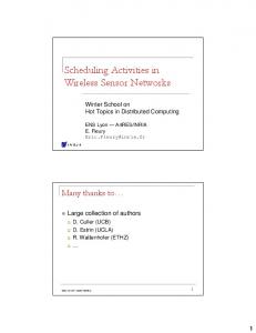
Figure 1.1: Four nodes (circles) communicate through three links (solid line) with controllable link capacities. The thickness of the lines corresponds to the capacity. The three leftmost nodes desire to send as much data as possible to the rightmost node. (a) When the network is not optimized, for instance allocating equal capacity to all links, the link to the right is a bottleneck. (b) Through cross-layer optimization, the link to the right is assigned more resources allowing more data to be transferred from nodes in the left side to the right side. The bottleneck link has been relieved. The example was taken from [2].

between a source and a destination, such as in cellular-relaying networks, or may also be source of their own data traffic, such as in ad hoc multi-hop networks. Traditionally, the functionality required to support end-to-end communication has been structured into distinct components, or layers, each responsible for a specific functionality. Layers are treated more or less separately and logically stacked on top of each other so that the higher layers can use the functionality provided by the lower layers without knowing their inner workings. This approach guarantees high modularity and simplifies both the design and the maintenance of the network. However, by allowing the layers to cooperate more closely and viewing the stack as a flexible structure, there could be performance benefits. This form of cooperation can be achieved through cross-layer optimization. A large body of the literature, see e.g. [3, 4, 5] and references therein, advocates cross-layer optimization as a powerful framework for the systematic design of networking protocols with performance guarantees. The drawback with this increased entanglement is that the design probably has to be redone if one layer is changed. Thus, the performance is improved at the expense of greater complexity. In some situations, cross-layer design may induce to a large number of new interactions among layers to the extent that layers may start working “against” each other, leading to worse practical performance than in a layered network, see e.g. [6]. The problem is typically formulated as a network utility maximization of the form maximize subject to

P ui (si ) Pi i∈I(l) si ≤ cl smin ≤ si ≤ smax

∀l ∀i.

(1.1)

Here, si is the communication rate for source-destination pair i, and the function ui (si ) describes the utility of pair i to communicate at rate si . Each logical link l is characterized by a capacity cl describing the sustainable data traffic. If I(l) denotes

1.1. Resource Management in Communication Systems

5

4

0.74

3.5

0.72

x 10

Link C −− D

3

0.7 2.5 Link rates [bps]

Total utility

0.68 0.66 0.64

2

1.5

0.62 1 0.6

Link A −− C Optimal Primal Decomposition Dual Decomposition

0.58

0

200

400 600 Iteration time t (at MAC−PHY layer)

800

0.5

0

1000

Link B −− C

0

200

(a) Network utility.

Optimal Primal Decomposition Dual Decomposition


800

1000

(b) Link-rates.

4

2.5

x 10

2 End−to−end rates [bps]

Rate S CD

8000 6000

1.5 4000 2000

1

Rate S AD 0.5

0

Rate S BD

0

200

0

5

10

15

20

Optimal Primal Decomposition Dual Decomposition


800

1000

(c) End-to-end source rates.

Figure 1.2: Two techniques, primal decomposition and dual decomposition, are used to optimize the operation of the network in Figure 1.1 assuming wireless links among nodes.

P the set data flows traversing link l, the inequality i∈I(l) sp ≤ cl states that the total traffic across a link cannot exceed its capacity. Solving the optimization problem (1.1) gives the optimal network performance, and the associated resource allocation. Such insight is useful for performance analysis and network dimensioning tasks. However, a more remarkable use of the network utility maximization framework is optimal protocol design. Kelly et al. [7] were the first to show that the network optimization can be performed distributively and that the components of such a distributed performance optimization maps onto idealized operation of TCP clients and active queue management schemes (see also [8]). It has been demonstrated that most of the common TCP/AQM variants correspond to different ways of solving the optimization problem (1.1). Now, different distributed optimization algorithms suggest different protocol solutions for achieving the optimal network operation. Figure 1.2 shows how problem (1.1) is solved for the network illustrated in Figure 1.1 assuming wireless links affected by path loss and shadow fading. The example shows two solution approaches based on primal and dual decomposition, respectively. Both solutions lead to the global optimum operating point, but with very different protocol dynamics and time-scales updates.

6

Introduction

Several contributions in this thesis consider the extension of the NUM framework to wireless systems, where the intricate resource couplings create many new theoretical and practical challenges.

1.1.2

Wireless Sensor Networks

Recently, a strong interest raised in migrating substantial parts of the traditionally wired industrial infrastructure to wireless technologies to improve flexibility, scalability, and efficiency. A critical requirement for applications related to industrial monitoring and control is timely and reliable data delivery, for instance for guaranteeing the performance of closed-loop controllers. Although industrial wireless is almost a hundred years old [9], the emergence of low-cost and low power radios along with the recent surge in research on wireless sensor networks and networked control raises expectations of a much wider deployment [10]. One of the main industrial concerns about a larger investment in wireless technologies has been the absence of networking standards (alongside with security concerns and the lack of proven operational reliability and latency). This has been acknowledged by major standardization bodies and automation system vendors, and several standards for industrial wireless networks are developed. The first of these to be finalized, wirelessHART, was accepted in the fall of 2007 and is now publicly available [11]. Designed to be an easy-to-use wireless mesh networking protocol leveraging on advanced techniques, such as time diversity, frequency diversity, path diversity and power diversity, WirelessHART achieves the level of reliability and latency required to support advanced process monitoring and control applications [12]. An important contribution in this thesis is to study real-time resource scheduling problems for delay sensitive applications, focusing on the design of optimal scheduling algorithms which comply with the WirelessHART standard.

1.2

Thesis outline and contributions

In what follows, we present the outline and contributions of the thesis in more detail.

1.2.1

Chapter 2

This chapter presents the basic assumptions and models used throughout the thesis.

1.2.2

Chapter 3

This chapter collects background information related the mathematical techniques and algorithms studied in the thesis. Starting from a rather general formulation of network utility maximization problems, we analyze the impact of the modelling assumptions on the problem structure. Then, three decomposition techniques for convex optimization are reviewed: primal, dual and prima-dual. As we shall see,

1.2. Thesis outline and contributions

7

these methods suggest layered, but loosely coupled, network architectures and protocols design and provide the guidelines for distributed cross-layer protocol design. This chapter is partially based on: B. Johansson, P. Soldati, and M. Johansson. Mathematical decomposition techniques for distributed cross-layer optimization of data networks. IEEE Journal on Selected Areas in Communications, 24(8):1535–1547, August 2006

1.2.3

Chapter 4

This chapter presents novel results on distributed cross-layer design for joint optimization of transport and physical layers in mobile ad hoc networks. Compared to the solution alternatives, the proposed approach has several attractive features: it adheres to the natural time-scale separation between rapid power control updates and slower end-to-end rate adjustments, and uses simplified power control mechanisms with reduced signalling. To validate the potential benefits of this approach, we present a detailed implementation of a cross-layer networking stack for DS-CDMA ad-hoc networks in the network simulator ns-2. Several critical issues arising in the implementation, but are typically neglected in the theoretical design, are described and the solution alternatives are compared in simulations. The material presented in this chapter is based on the following publications: P. Soldati, L. Balucanti, M. Belleschi, A. Abrardo, and M. Johansson. Respecting time-scales and reducing overhead: a novel cross-layer protocol design for MANETs. IEEE/ACM Transactions on Networking, 2009. (submitted) P. Soldati and M. Johansson. Reducing signaling and respecting time-scales in cross-layer protocols design for wireless networks. In Proc. of the IEEE Global Communications Conference (Globecom), Honolulu, Hawaii USA, Dec. 2009 M. Belleschi, L. Balucanti, P. Soldati, M. Johansson, and A. Abrardo. Fast power control for cross-layer optimal resource allocation in DS-CDMA wireless networks. In Proc. of the IEEE ICC International Conference on Communications, Dresden, Germany, June 2009

1.2.4

Chapter 5

In this chapter we present a novel mathematical framework for distributed optimization of end-to-end bandwidth sharing, transmission scheduling and power control in wireless systems. The optimization involves the operations at transport, data link and physical layer. The solution approach is quite general and allows to tackle the transmission protocol design of a large class of systems that support scheduled medium access, either over time, frequency or a combination of them. We will show in examples how the theoretical achievements apply to the design of S-TDMA wireless mesh networks or to OFDMA-based networks.

8

Introduction The following publications provide the cornerstones for this chapter:

P. Soldati, B. Johansson, and M. Johansson. Distributed cross-layer coordination of congestion control and resource allocation in S-TDMA wireless networks. Wireless Networks, 14(6):949–965, December 2008 P. Soldati and M. Johansson. A low-signalling scheme for distributed resource allocation in multi-cellular OFDMA systems. In Proc. of the IEEE Global Communication Conference (Globecom), New Orleans, LA USA, Dec. 2008 P. Soldati, B. Johansson, and M. Johansson. Proportionally fair allocation of end-to-end bandwidth in STDMA wireless networks. In Proc. of the 7th ACM MobiHoc International Symposium on Mobile Ad Hoc Networking and Computing, pages 286–297, Florence, Italy, May 2006 P. Soldati, B. Johansson, and M. Johansson. Distributed optimization of endto-end rates and radio resources in WiMax single-carrier networks. In Proc. of the IEEE Global Communications Conference (Globecom), San Francisco, CA, USA, Dec. 2006

1.2.5

Chapter 6

Originally driven by the desire of analyzing the techno-economic feasibility of cellular-relaying networks, this chapter proposes a novel cross-layer resource allocation model for wireless mesh networks, based on average interference and ideal rate adaptation for the physical layer, time-shares for the medium access layer, and fluid-flows for the transport and network layer. We formulate a centralized social welfare maximization problem, where the overall problem of allocating time-shares and selecting routes and link rates is non-convex. We also propose an iterative algorithm for solving the problem, based on a novel approximation of the physical layer. We prove analytically that each iteration consists of a convex subproblem, that the series of subproblems is convergent, and that it converges to the global optimum in case the route selection is not included in the problem formulation. The material in this chapter is based on the following publications: B. Timuş, P. Soldati, J. Zander, and D. Kim. Cross-layer resource allocation model for cellular-relaying network performance evaluation. IEEE Transactions on Vehicular Technology, July 2009. (submitted) Bogdan Timuş and Pablo Soldati. A joint routing-MAC model for cellularrelaying networks. In Proc. of the IEEE 19th International Symposium on Personal, Indoor and Mobile Radio Communications PIMRC, Cannes, France, Sept. 2008. (It has received the “MAC track best paper award”) Bogdan Timuş and Pablo Soldati. Cellular-relaying network dimensioning with cross-layer resource allocation. In Proc. of the IEEE 19th International Symposium on Personal, Indoor and Mobile Radio Communications PIMRC, Cannes, France,

1.2. Thesis outline and contributions

9

Sept. 2008 B. Timuş, P. Soldati, and J. Zander. Implications of fairness criteria on the techno-economic viability of relaying networks. In Proc. of the IEEE Vehicular Technology Conference (VTC), Barcellona, Spain, April 2009

1.2.6

Chapter 7

In this chapter we address the joint link scheduling and channel hopping problem for networks operating according to the recent WirelessHART standard. We consider a critical functionality for wireless networks deployed for industrial monitoring and control, so-called convergecast, in which data from a set of sources is routed toward one data sink. It turns out that the routing structure plays a fundamental role to achieve jointly time- and channel-optimal scheduling policies. Specifically, we will provide lower bounds on the minimum convergecast schedule length and bounds on the minimum number of channels for linear and tree routing structures. For networks with line and balanced complete m-ary tree routing topologies, we present jointly time- and channel-optimal scheduling policies taking into account different packet buffering capabilities. For networks with general tree routing topology, we first present time-optimal scheduling policies requiring only single-packet buffering capability. Then, we establish the lower bounds on the number of channels for time-optimal convergecast under different packet buffering capabilities, and present a heuristic algorithm for time- and channel-optimal convergecast scheduling. We further investigate the channel constrained convergecast problem, that is , given any fixed number of channels we design scheduling policies are able minimize the convergecast time, thereby enabling to explore the tradeoffs between the number of time slots and channels needed to complete convergecast. This chapter is based on the following publications: H. Zhang, P. Soldati, and M. Johansson. Optimal link scheduling and channel hopping in wirelessHART networks. ACM Transactions on Sensor Networks, October 2009. (submitted) P. Soldati, H. Zhang, and M. Johansson. Deadline-constrained transmission scheduling and data evacuation in wirelessHART networks. In Proc. of the European Control Conference (ECC), Budapest, Hungary, August 2009 H. Zhang, P. Soldati, and M. Johansson. Optimal link scheduling and channel assignment for convergecast in linear wirelessHART networks. In Proc. of the IEEE WiOpt, Seoul, Korea, June 2009 J. Pesonen, H. Zhang, P. Soldati, and M. Johansson. Methodology and tools for controller-networking co-design in wirelessHART. In Proc. of the 14th IEEE International Conference on Emerging Technologies and Factory Automation (ETFA), Mallorca, Spain, September 2009

10

1.2.7

Introduction

Chapter 8

This chapter summarizes the contribution of this thesis. It gives the main conclusions and suggests the natural steps to continue the work in this thesis.

1.2.8

Other Publications

The following publications are not covered in this thesis, but they have influenced the contents. G. Fodor, M. Johansson, and P. Soldati. Near optimum power control in CoMP systems under fairness constraints. In Proc. of the IEEE Global Telecommunications Conference (Globecom), Honolulu, Hawaii USA, dec. 2009 G. Fodor, M. Johansson, and P. Soldati. Near optimum power control and precoding under fairness constraints in network MIMO systems. International Journal of Digital Multimedia Broadcasting, March 2010. (To appear) P. Park, P. Di Marco, P. Soldati, C. Fischione, and K. H. Johansson. A generalized Markov model for effective analysis of slotted IEEE 802.15.4. In Proc. of the IEEE MASS, Macau SAR, P.R.C., October 2009. (It has received the “MASS best paper award”) P. Soldati and M. Johansson. Network-wide resource optimization of wireless OFDMA mesh networks with multiple radios. In Proc. of the IEEE International Communication Conference (ICC), Glasgow, Scotland, June 2007 S. Loretti, P. Soldati, and M. Johansson. Cross-layer optimization of multi-hop radio networks with multi-user detectors. In Proc. of the IEEE Wireless Communications and Networking Conference (WCNC), New Orleans, La, March 2005

Chapter 2

Resource Allocation Models

T

his chapter presents the mathematical models for communication networks used throughout this thesis. Although all these models focus on the interplay between the radio resource management and the networking operations, their aim can be quite different: some are detailed models describing fine-grained resource allocation decisions critical to protocol design, while others are high-level models useful for network dimensioning and performance analysis. The detailed outline of this chapter is as follows. Section 2.1 shortly reviews various modelling approaches commonly used in the literature. A cross-layer model for the systematic design of distributed transmission protocols of communication networks is described in Sections 2.2-2.3. A simplified cross-layer resource allocation model suitable for network design and off-line evaluation of the network performance is presented in Section 2.4 Finally, Section 2.5 proposes a model suitable for realtime resource scheduling.

2.1

Modelling of Communication Systems

A reliable model shall provide the link between the physical characteristics of a system and the mathematical techniques for its analysis. Detailed modelling of complex systems is often overwhelming and rather complicated as it requires to balance between accuracy and simplicity, i.e. between the desire of precisely describing as many aspects as possible and the will (or need) of formulating tractable problems. Two important issues emerge: what is the purpose of the model and which level of abstraction should be used? Since the field of wireless communications embraces several non-trivial disciplines, such as information theory, communication theory, resource management, optimization etc., the answer to this question may change case by case. Finding the best compromise among these aspects is therefore essential. The classic information theoretic approach starts from the physical aspects of the radio propagation to arrive to an input/output formulation of the wireless channel as a linear time-varying system, see e.g. [34] and references therein. Starting from Claude Shannon in 1949 [35], information theory used this approach to 11

12


characterize the limits of reliable communication, the so-called channel capacity, of various wireless channel models. The basic idea is that through intelligent coding of the information, one can communicate at a strictly positive rate with vanishing error probability. The capacity of the wireless channel defines the theoretical rate limit at which this operation can be done, i.e. communication at higher rate makes impossible to drive the error probability to zero. In some cases, such as for the IS-95 Code Division Multiple Access (CDMA) standard, this approach led to a significant impact in practical applications [34]. The information-theoretic analysis feeds into the other disciplines by specifying the relationship between the resource allocation and the resulting link-rates. This macroscopic view of the network operation is preferred, for instance, in the design of transmission protocols that regulate the users access to the wireless medium. Similarly, from a networking prospective a detailed model of the data traffic and the way data flows are routed through the network is more relevant than dealing with the specific details of the data transmission over the physical channel. Nevertheless, the achievable source-destination rates will depend on both the routing of data trough the network and the sustainable link-rates on the wireless channel. Modelling choices could be also driven by application requirements. For instance, streaming and voice services, or industrial process monitoring and control applications, are typically delay sensitive, therefore it is essential to model the packet delay distribution. In what follow, we will recall the basic notions of the information-theoretic analysis and describe how they feed into models for an optimization framework that aim to capture the coupling among different network operations into resource constrains.

2.1.1

The OSI Reference Model

Network functionalities and services are commonly classified through the well-known Open System Interconnection (OSI) network model. The OSI reference model establishes a 7-layer protocol stack where each layer defines the specifications for a particular network aspect and provides services to the upper layers. Figure 2.1 shows the layered hierarchy of the OSI network stack where: • The Physical layer deals with signal transmission over the channel. • The Data Link layer provides the abstraction of “link” and the ability to transmit raw of bits over the channel. This layer consists of two sub-layers: - Logical Link Control (LLC) multiplexes protocols running at higher layers. It optionally provides flow control, acknowledgment, and error recovery. - Medium Access Control (MAC) hosts the routines that regulate the access to the physical medium, which can be either centralized or decentralized. • The Network Layer introduces the concept of source-destination path and handles the routing of data flows through the network. • The Transport layer provides a virtual end-to-end channel.

2.1. Modelling of Communication Systems

13

Source Node

Destination Node Application Protocol

Application

Presentation Protocol

Presentation

Application Presentation

Session Protocol

Session

Transport Protocol

Transport

Session Transport

Network

Network

Network

Network

Data Link

Data Link

Data Link

Data Link

Physical

Physical

Physical

Physical

Communication Subnet Boundry

Figure 2.1: ISO/OSI reference model.

• The last tree layers, less significant to the scope of the thesis, create sessions between users, structure the data to enable communication among devices using different data formats, and define the user applications, respectively. The OSI model provides modularity and simplifies the network design by letting layers at the same level interact with each other without knowing the operation at the lower levels. This per-layer communication encourages the optimization of each layer separately in a layered fashion. In many systems, however, there exists a strong inherent coupling between the operation at different layers. For instance, in wireless networks adjusting the resource allocation at the physical and MAC layers, such as transmit power or transmission rights, changes the average link-rates, influences the optimal routing, and alters the achievable performance. Off-line optimization returns network settings that can very well be implemented in the layered model. However, it is really when we try to design protocols that we see these interactions coming into play in a way that needs coordination across layers in a cross-layer fashion. A model for these dependencies will be developed next.

2.1.2

Network Topology

We consider a network consisting of a constellation of geographically distributed radio units, i.e., nodes. Each node is assumed to have infinite buffering capacity and can transmit, receive and relay data to other nodes over wireless multi-hop links. Unless differently stated, nodes are assumed to be at fixed positions in the plane. We describe the network topology by a directed graph G = (V, E), with nodes labelled n = 1, . . . , N and (logical) radio link labelled l = 1, . . . , L. A link is represented by an ordered pair (i, j) of distinct nodes, i.e., an arc in the topology graph. The presence of link (i, j) means that the network is able to send data from node i to node j. Associated with each node n are two sets, namely O(n) and I(n), collecting the outgoing and incoming links to the node, respectively.

14

2.2


The Physical and Data Link (MAC) Layer Model

The purpose of this section is to characterize the interplay between data link and physical layers of several communication systems. The main outcome will be the theoretically achievable link capacity, and we will introduce the notation c ∈ C,

(2.1)

for indicating that the link-rate vector c belongs to the appropriate multi-user rate region C. The shape of the multi-user rate region depends on which underlying MAC and PHY-layer technologies are used. To be able to optimize over the link-rate vectors c, we often need to explicitly model how c depends on the resource allocation. In some cases, such as optical networks, the links capacity is fixed (typically the physical limit of the deployed cables), and the region C takes the simple form C = {cl | cl = cl,max ∀ l}. In wireless systems, however, the achievable link-rates are not fixed à priori but depend in a non trivial way on the allocation of the communication resources at both data link and physical layer, such as time slots in a transmission schedule, transmission power, channels, rate, coding and modulation etc.. Moreover, the quality of the wireless channel is typically not constant, neither over time nor over the frequency domain. Besides the deterministic (distance-based) signal strength attenuation1 , abrupt and unpredictable changes occur due to both large-scale fading2 or small-scale fading3 . Starting from a simple baseband signal model, in what follows we derive the Shannon-limit for the transmission rate and we discuss both continuous and discrete rate mapping. Finally, we demonstrate how these basic concepts can be applied to define the multi-user capacity region of several technologies, including Code Division Multiple Access (CDMA), Time Division Multiple Access (TDMA), Orthogonal Frequency Division Multiplexing (OFDM) and Orthogonal Frequency Division Multiple Access (OFDMA)4 .

2.2.1

Signal Model

We consider a Gaussian frequency-selective interference channel composed by multiple links simultaneously sharing the same physical resources, e.g., time and bandwidth, as in Figure 2.2. We focus on transmission techniques where no interference cancellation is performed and each receiver treats multiuser interference as additive noise. No multiplexing strategy is imposed à priori so that, in principle, all users interfere with each other. To avoid excessive signaling and coordination among users, 1 Path loss: The theoretical attenuation of the signal radiated by a transmitter in free space that would occur if all aleatoric factors were disregarded, i.e. it depends on frequency and distance. 2 Slow fading: Shadowing, or large-scale fading, represents the average signal power attenuation due to obstructions within the environment between transmitter and receiver, such as terrain contours, forests, clumps of buildings, or movements of users over large areas. 3 Fast Fading: Multi-path fading, or small-scale fading, occurs due to small movements or obstacles, on the order of the signal wavelength, and can dramatically affect both amplitude and phase of the received signal. 4 Although not included in this thesis, the model extends to multi-user detectors, see e.g. [33].

2.2. The Physical and Data Link (MAC) Layer Model

15

Figure 2.2: Examples of interference caused by multiple access. The first case is the uplink of a cellular system, the second case is the uplink of a WLAN.

each link is assumed to perform encoding/decoding independently of the other links. Block transmissions are considered as a general framework embracing most current schemes like, e.g., TDMA, CDMA, or OFDM systems. We view each link as a single-user Gaussian channel transmitting an information symbol zl (eventually coded by means of pre-coding matrix), and adopt the baseband signal model y = Hz + w,

(2.2)

to describe the simultaneous transmission over L links. Here, H ∈ CL×L is the p ρ channel matrix, and Hlk = H lk / dlk denotes the channel frequency response between the transmitter (source) of link kth and the receiver (destination) of link lth, including distance based path-loss attenuation dρlk , with exponent ρ, and a normalized fading H lk ; y ∈ CL is the vector of received signals; and w ∈ CL is a zero mean circularly symmetric complex Gaussian white noise vector with covariance σl2 I. By expanding the signal model (2.2) in the form yl = Hll zl +

X

Hlk zk + wl

l = 1, . . . , L,

k6=l

it is easy to recognize the direct channels in the diagonal elements of H, and the interference channels in the off-diagonal elements. The power allocated to the transmission of zl is denoted by Pl = E{|zl |2 }. We will consider, for instance, a) Per-link peak-power constraints in the form Pl ≤ Plmax

l = 1, . . . , L,

(2.3)

b) Per-node total power budget in the form X

l∈O(n)

Pl ≤ Pntot

n = 1, . . . , N.

(2.4)

16

2.2.2


Achievable Transmission Rate

Given the signal model in (2.2), the achievable link transmission rate is defined as the maximum information rate, treating the other received signals as additive noise [36]. Under certain idealized conditions (e.g., ideal channel estimation, asymptotically long codewords, error-free link adaptation, etc.), the spectral efficiency achieved by the lth user with vanishing error rate, i.e. the Shannon-limit, is cl (p) = log2 (1 + γl (p))

[bps/Hz] ∀ l,

(2.5)

where p = (P1 · · · PL )T is the power allocation vector, and γl (p) denotes the Signalto-Interference plus Noise Ratio (SINR) for the lth link defined as γl (p) =

σl2

|H |2 P Gll Pl P ll l 2 = 2 P + k6=l |Hlk | Pk σl + k6=l Glk Pk

∀ l.

(2.6)

Here, Glk = |Hlk |2 denotes the effective gain between the transmitter of link j and the receiver of link l (including path-loss, fading, as well as the effects of coding, spreading gain etc., see e.g., [37]). Equation (2.5) defines a mapping from the power allocation p, via the resulting SINR at the receiver, to the achievable data rate. Under the Shannon assumptions, bits transmitted at rate (2.5) are received with asymptotically small bit error rate (BER), cf. [37]. Conversely, cl can be read as the maximum data rate that meets a given BER requirement of a modulation scheme, cf. [38, 39]. Most practical communication schemes will achieve substantially lower rates, and the effectively achievable spectral efficiency can be quantified as cl (p) = log2 (1 + Kl γl (p))

[bps/Hz] ∀ l,

(2.7)

where Kl ≤ 1 models the SINR-gap for a specific coding and modulation5 [38]. Adaptive coding and modulation schemes adjust the transmission format to the sustainable SINR, providing high spectral efficiency by transmitting at high rate under favorable channel conditions or reducing the throughput when the channel degrades. The mapping (2.5) is difficult to realize in practice. Firstly, the Shannon capacity is achievable only in the limit6 . Secondly, the continuous SINR-rate mapping would require an infinite number of codes. Practical coding schemes, however, rely upon finite order constellations of symbols with limited coding block size, cf. [41]. To capture this effect, the rate curves can be modelled as a piecewise constant functions of the sustainable SINR as cl = ctgt,j l

if

γltgt,j ≤ γl (p) < γltgt,j+1

∀ l,

(2.8)

5 For ease of notation, the theoretical results presented in this thesis refer to the case K = 1. l Nevertheless, numerical examples and simulations may use different values of Kl . 6 Data should be split in packets with variable length and repacked with new headers for re-sequencing the original information at the receiver side, see e.g. [40] for a detailed discussion. Although we do not model this aspect, Chapter 4 evaluates in simulations the impact of packet with fixed payload size for systems using continuous rate mapping.

6

6

5

5 Transmission rate [bits/s]

Transmission rate [bits/s]


4

3

2

1

0

17

4

3

2

1

0

5

10

15 SIR

20

25

(a) Multiple rate formats.

30

0

0

5

10

15 SIR

20

25

30

(b) Single rate format.

Figure 2.3: Example of piecewise affine functions for multi-level rate allocation.

where ctgt,0 = 0, γltgt,0 = 0 and γltgt,j < γltgt,j+1 , where ctgt,j and γltgt,j denote l l the jth discrete rate format and the associated SINR, respectively, as in Figure 2.3. In practice, for a given BER, the number of constellation points is adapted to the channel state, i.e. it is decreased when the receiver is in deep fade, or increased if the channel state is sufficiently good, cf. [40, 42, 43, 44]. A special case of (2.8) is when links offer a single rate format ctgt = log2 (1+γltgt ) l tgt if the SINR at the receiver exceeds a communication threshold γl , eventually the same for each link/node. To capture this effect, we rewrite (2.8) as ( tgt ctgt l , if γl (p) ≥ γl cl = (2.9) 0, otherwise. The model implicitly assumes fixed target decoding error probability, coding, and modulation scheme. The only degree of freedom is the transmission power adaption7 .

2.2.3

Multiple Access Interference (MAI)

The communication quality over a certain link depends on its own transmission power, but also on the transmission power of other active links, which are experienced as interference. The impact of the interference on the link quality (or, more generally, on the quality of service QoS) can be read, for instance, in terms of SINR degradation. Interference mitigation (or rejection) can be improved by ensuring data transmission diversity, for instance via coding, or over time and frequency. Code Diversity via CDMA CDMA systems, along with Spread Spectrum (SS) techniques, are widely used to mitigate interference by ensuring code diversity through (theoretically) orthogonal 7 In essence, we will show numerical results only for this special case, though we would only need this restriction in decentralized schemes.

18


codes assigned to users. We will consider a CDMA systems with nodes equipped with omnidirectional antennas, and with a matched filter and a CDMA spreading sequence preassigned to each link8 . To account for the spreading gain S, we rewrite the SINR in (2.6) using Glm = G′lm /S for m 6= l, and σl = Neq B. Here, B = W/S is the system bandwidth normalized to the spreading gain, and Neq models the noise figure and thermal noise at the receiver. The achievable link-rate becomes cl (p) = B log2 (1 + γl (p))

[bps] l = 1, . . . , L.

(2.10)

If a power budget is not imposed, the achievable rate region resulting from (2.10) may be unbounded (an example is the rate maximization problem where a single link is allowed to use infinite power). In practice, however, nodes have a limited power budget9 which can be enforced either on links through (2.3) or on nodes through (2.4). Therefore, the multi-user capacity region takes the following form CCDMA , {c | cl satisfies (2.10) ∀l, subject to (2.3) or (2.4)}.

(2.11)

Time Diversity via TDMA and S-TDMA The simplest way to provide time diversity and interference rejection is by time sharing the system resources (bandwidth, ect.) among users. Time division multiple access (TDMA) guarantees a time orthogonal resource allocation by letting a single user to transmit at any given time. Time is slotted in interval of fixed duration, referred to as time slots. A transmission schedule describes the allocation of resource blocks to the users in terms of time slots, transmission power and rate formats. Scheduling users to access the medium is particularly efficient to enhance the achievable multi-user capacity region when the impact of multiple access interference is strong, as illustrated in the following example. Example 2.2.1. Figure 2.4 pertains to the rate region of a two-link wireless system subject to individual peak-power constraints, and operating in the highSINR regime (upper row) and low-SINR regime (lower row), respectively. The leftmost picture at each row shows the achievable instantaneous rate region under continuous power and rate adaption, while the middle picture illustrates the (finite) set of feasible rates (marked by dots) for a discrete rate allocation. The rightmost figures compare the instantaneous rate region with the longterm average rate regions achievable by combining discrete rate allocation with time-sharing (dark blue region). In the high-SINR case, the quantization effect from using a finite set of rates forces the long-term rate region to be strictly smaller than the instantaneous rate region under continuous power and rate adaption. In the low-SINR regime, scheduling is instrumental for mitigating 8 We further assume perfect self-interference cancellation and nodes able to transmit and receive simultaneously. Such assumption is suitable through RF isolators and echocancelers, coupled with base-band digital filtering, see [45] and references therein. 9 As we shall see later, power budget may be replaced by a global power minimization problem.


19

Figure 2.4: Rate region under high-SINR and low-SINR regimes.

multi access interference and achieving good average transmission rates on both links. Thus, while continuous rate and power allocation are beneficial when all users experience good channel quality, scheduling is instrumental to protect users from bad performance in case of high interference. TDMA, however, can be wasteful since in practice one may maintain multiple transmissions without causing too much interference to each other. Spatial reuse TDMA (S-TDMA) enables multiple users to access the channel simultaneously if they are sufficiently separated apart [46]. Moreover, half-duplex technology refrains nodes from receiving and transmitting signals at the same time. This results in a combinatorial constraint on which links that can be activated simultaneously, which complicates the scheduling and resource allocation problem considerably. In fact, the combinatorial nature of this problem is sometimes so dominant that researchers disregard the power control all together and focus solely on the scheduling aspect. When a link is assigned to transmit in a time slot, the rate selection scheme (2.8) leads to a finite number of achievable link-rate vectors c(k) = (c1 . . . cL )

k = 1, . . . , K,

20


where cl ∈ {0, ctgt,1 , . . . , ctgt,J−1 } is any of J transmission formats. By time-sharing among link-rate vectors, the following polyhedral rate region can be achieved n o X X CS-TDMA , c = αk c(k) | αk ≥ 0, αk = 1, k = 1, . . . , K . (2.12) k

k

The time-sharing coefficients αk represent the fraction of schedule in which the linkrate vector c(k) is activated. Although K may be as large as J L , interference and the half-duplex restriction drastically reduce the number of link-rate vectors that can be supported. Moving from a saturated traffic model to delay sensitive traffic, the long-term average performance should be replaced with more appropriate metrics. This subject will be discussed in Section 2.5 and Chapter 7.

2.2.4

Frequency Diversity via OFDM and OFDMA

To capitalize on the frequency-selectiveness of the fading channel, OFDM technique converts the channel into a set of orthogonal, narrowband, flat fading sub-channels. The system bandwidth W of a block of transmission is divided into F equally sized and non-overlapping sub-carriers labelled f = 1, . . . , F . The propagation channel is assumed to be slowly time-varying and frequency selective, with the channel coherence bandwidth larger than the bandwidth of each sub-carrier. Frequency diversity is obtained by letting users transmit the data over different sub-carriers. Sub-carrier reuse among users creates multiple access interference10 . The signal model in Section 2.2.2 can be extended to each sub-carriers, leading to the definition of the SINR of link lth over sub-carrier f th as γlf (pf ) =

G P P llf lf σlf + m6=l Glmf Pmf

∀l, f,

(2.13)

where pf = (P1f · · · PLf )T is the channel power vector, Glmf is the channel gain between the transmitter of link m and the receiver of link l, σlf be the thermal noise power at the receiver. For convenience, we define a global power vector p = vec(p1 . . . pF ). Thus the total achievable transmission rate on link l becomes P cl = W F −1 f log2 (1 + γlf (pf )) ∀ l. (2.14)

Alternatively, by using the discrete rate selection (2.8) to find the sustainable transmission format clf of each link in each sub-carrier, the achievable rate on link l is cl =

PF

f =1 clf

∀ l,

(2.15)

which leads to a finite number of link-rate vectors c(k) = (c1 . . . cL )

k = 1, . . . , K.

10 Examples in this sense are multi-cell OFDMA cellular networks with reuse factor one (see e.g. LTE or WiMAX), where each subcarrier is assigned to at most one user within each cell.

2.3. The Transport and Network Layers

21

Similarly to the S-TDMA case, time-sharing between link-rate vectors allows to achieve the following polyhedral rate region n o X X COFDMA , c = αk c(k) | αk ≥ 0, αk = 1, c(k) s.t. (2.14) − (2.15)∀k (2.16) k

k

where the number of possible link-rate vectors K may be as large as (J + F − 1)L , although the number of possible (L × F ) matrix combinations resulting from J multi-rate formats is J L×F . Most networks, however, will support substantially fewer link-rate vectors due to interference and other technological constraints.

2.3 2.3.1

The Transport and Network Layers The Transport Layer

At the transport layer, we use a fluid flow model for the user data traffic, i.e. we assume saturated (bit-level) traffic where sources have full data buffers, and ignore the delay distribution of the individual packets. Source-destination pairs are labelled by integers i = 1, . . . , I and communicate at average rate si [bps]. Each pair shares (or eventually competes for) the end-to-end resources with all other users in the network. Defining S as the set of feasible end-to-end rates, we use the notation s∈S

(2.17)

to denote that the rate vector s is feasible. The set S typically implies an upper and a lower bound on the end-to-end-rate si , i.e. S = {s | si,min ≤ si ≤ si,max ∀i}. A critical aspect of transport layer models is to describe the utility that users have of being able to communicate a given end-to-end rate s. This is typically described by a per-user utility function ui (si ). We will discuss various utility in more detail in Chapter 3, but note that in many cases the performance of the network is directly related to the end-to-end rates. Thus, it is natural to find the best rate vector s that can be supported, e.g. the maximum throughput. In other cases, the end-to-end rate vector s also allows to abstractly model the stationary behavior of congestion control protocols, e.g. the bandwidth sharing of TCP/IP networks.

2.3.2

The Network Layer

Routing protocols determine the routes along which data is forwarded from source to destination, and regulates the amount of data sent along each individual paths. In this way, the routing also limits the achievable end-to-end rates. In most models for communication networks, each source-destination pair is supported by only one route. A counter example in this sense is the soft handover in CDMA types of systems; another one is the case of a heterogeneous environment in which terminals with multiple air interfaces can be connected to several access networks at the same time. Cooperative relaying and network coding are example of theoretic concepts

22


in which data may follow parallel tracks. Multicommodity flow models have been widely used in the literature of network routing and optimization to address these concepts, see e.g. [47]-[50] or more recently [51]. A Multicommodity Flow Model: The classic multicommodity flow model assumes lossless flows across links and routes the data traffic through several parallel paths at each intermediate node. Flows with the same destination are considered as a single commodity regardless of their sources. Let the destination nodes be labelled d = 1, . . . , D where D ≤ N . For each destination d, we define a source-sink (d) vector s(d) ∈ RN whose nth (n 6= d) entry, sn , denotes the non-negative data rate injected to the network at node n (the source) destined for node d (the sink). P (d) (d) The flow conservation law imposes the sink flow sd = − n6=d sn at the destina(d)

tion node. Let xl be the amount of traffic on link l destined for node d, and call x(d) ∈ RL the flow vector for destination d. At each node n, the components of the flow vector and the source-sink vector for the same destination satisfy the following flow conservation law X (d) X (d) ∀(d, n), xl − xl = s(d) n l∈O(n)

l∈I(n)

which can be compactly written as hd (x(d) , s(d) ) , Ax(d) − s(d) = 0

∀d,

where hd : RL × RN 7→ RN , and A ∈ RN ×L is the node-arc incidence matrix whose entry Anl is 1 if node n is the transmitter of link l; -1 if node n is the receiver of link l; and zero otherwise. Finally, given the link-rate vector c = [cl ], the total amount P (d) of traffic on each link, i.e. tl = d xl , should not exceed cl . Altogether, the model imposes the following constraints on the variables x(d) , s(d) and c hd (x(d) , s(d) ) , Ax(d) − s(d) = 0 ∀d PD g(x, c) , d=1 x(d) − c 0 x(d) 0, s(d) d 0, c ∈ C ∀d,

(2.18)

where g : RLD × RN 7→ RL , the symbol denotes componentwise inequality, and d means componentwise inequality except for the dth component. A Multi-Route Selection Model: The multicommodity flow model is quite general and in essence it describes how the data flow is split at each node into multiple directions. In some cases, however, it is more natural to use a model that explicitly reveals the route selection. As an example, consider the optimal route selection problem in cellular-relaying network as exemplified in Figure 2.5. Here, some of the nodes are connected directly to the wired core network (i.e. are access points or base stations), some are using air interfaces to receive and forward data

2.3. The Transport and Network Layers PSfrag

23 routes links core

I terminals

relays

bases

Figure 2.5: I terminals are connected to the core network via R routes. Some routes may pass through relays, others go directly through the access points. A terminal can be connected through several routes; several routes can pass through the same (logical) radio link.

from other nodes (i.e. are relays), others are user terminals. Finding the optimal combination of routes from each terminal to the core network is instrumental for establishing the achievable system performance. In what follows, we present a model for load balancing across multiple fixed routes. For the sake of simplicity, each route is uniquely associated with a sourcedestination flow, with R(≥ I) denoting the number of possible routes. Let F ∈ RI×R be the flow-to-route incidence matrix, with Fir = 1 if the rth route carries data for the ith source-destination flow, and 0 otherwise. Let xr be the data flow through the rth route11 , the flow conservation at each node imposes the routing constraint12 : hi (x, s) ,

R X

Fir xr − si = 0,

i = 1, . . . , I,

(2.19)

r=1

where hi : RR × RI 7→ R, or in a compact matrix notation h(x, s) , Fx − s = 0.

(2.20)

Let R ∈ RL×R denote the link-to-route incidence matrix, with entries Rlr = 1 if the rth route passes through the lth link, and zero otherwise The vector of total traffic across links t = Rx is upper bounded by the capacity of the link gl (x, c) ,

R X

Rlr xr − cl ≤ 0

l = 1, . . . , L,

(2.21)

r=1

where gl : RR × RL 7→ R. Altogether, the model imposes the following constraints h(x, s) , g(x, c) , x∈X

Fx − s = 0 Rx − c 0 s∈S c ∈ C.

(2.22)

(d)

11 With an abuse of notation, here we use x with a different meaning. While x denotes the l traffic with destination d traversing link l, here xr is the rate associated with route r. 12 This constraint is written by assuming that each packet follows an unique route, i.e. no multiroute redundancy is used. Multi-routes could be used for forward error protection redundancy, as well as for retransmissions. In our model the transmission reliability is dealt with at the link (physical) level, i.e. per route segment only.

24


Remark 2.3.1. Note that the variable x has different interpretations in the two models: in the multicommodity network flow model, it describes how an aggregate flow is split in each intermediate node, while in the route selection model, its components correspond to the total load on the individual paths The Single Route Case: It is sometimes natural to keep the routes between the source-destination pairs fixed, and only allow the source rates to vary. If a routing algorithm is à priori run P so that each source i is associated with an unique route r we have s ≡ x (and i r r Fir = 1). Therefore, the total traffic across links is given by P tl = r Rli si and the network flow model imposes the following set of constraints g(s, c) , s∈S

2.4

Rs − c 0 c ∈ C.

(2.23)

A Simplified Model for Performance Analysis

When the model is not expected to support the design of algorithms to be implemented in real networks, a different (eventually simplified) approach can be applied. To overcome the redundance of details typical of protocol design, we propose a novel cross-layer radio resource model in which the resource allocation is treated in average sense. Compared to previous sections, this model does not provide any explicit time-slot structure, but time-slots are seen as continuous variables {αl }L l=1 ∈ [0, 1]. The MAC protocol creates mutual exclusion conditions on links, so that when two links cannot be activated at the same time, this will be reflected by a requirement on their assigned time-share fraction {αl }13 . The model is designed to estimate an upper bound of the network performance, not to be the basis for protocol design. Example 2.4.1. Uncoordinated Cellular Example: In a traditional single-hop cellular network, each base station is allocated a share of the total spectrum, and is delegated the responsibility of scheduling resources to the terminals connected to it. For the sake of simplicity, we exemplify the model for a network with frequency reuse one, such as HSPA. In a long term average (so as to ignore the specific, practical time slots) the following constraint can be written for each cell: X αl ≤ 1, ∀ cell n. (2.24) user l in cell n

The model can also be used for other fixed resource allocation schemes, such as the schemes proposed in the WINNER project for a two-hop cellular network [52, page 24]. It can easily be extended to systems with several carriers. 13 Unlike the previous model, in which the time-sharing coefficients were associated with a transmission vector, in this case each αl describes the transmission activity of a specific link.

2.4. A Simplified Model for Performance Analysis

25

th k-th link

h-th link

tk tl l-th link

rl

T RTS

CTS

Figure 2.6: A pathgain threshold T is used for the RTS/CTS link exclusion area.

An RTS-CTS Example: To improve the link quality for terminals located at the cell border, neighboring cells could coordinate the resource scheduling. Another way is to exploit the broadcast properties of the radio environment for coordinating the medium access, for instance by a RTS-CTS mechanism14 . RTS and CTS messages reserve resources within T dB “radio distance” from the transmitting and the receiving nodes, respectively. A boolean matrix B ∈ RL×L , called the link mutual exclusion matrix, is defined so that Blk = 1 if the kth link can not be active at the same time with the lth link, and Blk = 0 otherwise. Given the pathgain Grl tk between the transmitter of link k and the receiver of link l, the exclusion area in Figure 2.6 is mathematically expressed as: ( 1 if Gtl tk > T or Grl tk > T or k = l Blk = (2.25) 0 otherwise. This model recalls the protocol model used by Gupta and Kumar in [53]. Nonetheless, the exclusion area could be defined for each individual link, so that the robust links have a smaller exclusion area, as in cellular systems with fractional channel reuse [54, 55]. Unlike the uncoordinated cellular case, where each link uniquely belongs to a cell, in the RTS-CTS case a link may belong to several exclusion areas. For instance, in Figure 2.6 none of the links k and h may be active at the same time as link l, but they can be active at the same time if link l is inactive since they are not in each other’s exclusion areas. If we see αl as a transmission probability, and if the overhead due to signalling and collisions are ignored [56], then αl is upper bounded by the probability for all the links in the lth exclusion area to be silent: αl ≤

L Y

k6=l

(1 − Blk αk ) = 1 −

X

Blk αk + ∆.

(2.26)

k6=l

The term ∆ stands for the probability for two links k and h to belong to the lth exclusion area, but not to each others exclusion area. In the following we ignore 14 A Request To Send (RTS) message is broadcasted by the source node, which may reserve (block the medium). The destination node may answer with a Clear To Send (CTS) message, which reserves the medium around the receiver, and thus protects the reception.

26


these joint probability terms ∆ ≈ 0, and approximate the above expression by its linear part15 . Thus we generalize the constraint previously expressed for each cell, to a MAC constraint for each link: X fl (α) , αl + Blk αk − 1 ≤ 0, 0 ≤ αl ≤ 1. (2.27) k6=l

Active links use a constant transmission power Pl , i.e. no power control is employed. The bit-rate along a radio link is modeled based on the average interference created by the other links active at the same time. Then the link capacity is modeled as16 : Pl Gll , (2.28) cl (α) = min cmax , ζ1 W log2 1 + ζ2 I¯rl + σ 2 where I¯rl =

L X

(1 − Blk ) αk Pk Glk ,

k=1

is the average interference and cmax is the maximum link-rate. Here, ζ1 and ζ2 depend on the modulation scheme, channel coding, etc. Notice that in the RTSCTS model of the MAC layer, the closest interferers are always removed, since (1 − Blk ) = 0 if Glk > T 17 . Finally, total traffic through a link is upper bounded by the capacity of the link as gl (x, α) ,

R X

Rlr xr − αl cl (α) ≤ 0,

∀ l.

(2.29)

r=1

As a final remark, the MAC model could be extended with a constant term to account for the signaling overhead, or to cover systems where users are multiplexed in frequency or in a combination of time and frequency [57, 58], e.g. LTE or WiMAX.

2.5

A Model for Real-Time Resource Scheduling

The models discussed so far capture average link-rates and traffic flows in the network, and focus on mapping the resource allocation to the average long-term system performance. However, a growing number of applications, including wireless networks for industrial control, demands precise control over the real-time performance of individual packets. In what follows, we describe a mathematical programming model for transmission scheduling of deadline-constrained data transfers. This 15 By ignoring the signaling overhead, the total resource allocation is overestimated. By ignoring the joint transmission probabilities αk αh , the resource allocation is underestimated. 16 This expression should not be read as a time-average over peak rates in different time slots, but rather as a model accounting for the statistics of fading channel, retransmissions, etc. 17 T can be tuned so as to control the average interference I. ¯ An example of the effect of tuning T has on the network performance is given in [19].

2.5. A Model for Real-Time Resource Scheduling

27

model disregards multi-access interference and assumes that active links can transmit reliably at a single rate. The model will be the basis for the design of efficient radio resource scheduling algorithms proposed in Chapter 7. We assume a fixed network topology over time. Data packets d are produced at (d) (d) individual nodes18 vn,0 ∈ V at given times t0 . Associated to each data transfer is (d)

(d)

a deadline tf when the data has to be delivered at its destination node vn,f ∈ V. The problem is to construct a link schedule that delivers the data on time. The schedule assigns transmission rights to links. There are C channels for use in the network, and in each time slot t only one transmitter can send in each channel19 . Moreover, current radio platforms impose the limitations that a node cannot receive and transmit simultaneously, i.e. half-duplex constraints. Finally, we set a limit pn,max on the number of packets that can be buffered at node vn .

2.5.1

Time-Expanded Graphs and Dynamic Network Flows

One way to deal with network flows over time is to use time-expanded graphs GT = (VT , ET ) [59]. These are obtained from the network topology graph G = (V, E) via VT = {vn,t : vn ∈ V, 0 ≤ t ≤ T }, where vn,t is the t-th time copy of the node vn ∈ V and ET = {(vn,t , vm,t+1 ) : (vn , vm ) ∈ E}. We will use the shorthand notation lt ∈ ET to denote the t-th time copy of link l = (vn , vm ) ∈ E. A deadline-constrained flow on G can then be modelled as a classical network flow on the time expanded graph GT ; see Figure 2.7 for an illustration.

a

a0

a1

a2

b

b0

b1

b2

aT bT ...

c d

c0

c1

c2

cT

d0

d1

d2

dT

t=0

t=1

t=2

t=T

Figure 2.7: A simple network and the corresponding time-expanded graph. The grey arrows denote hold-over links. 18 With an abuse of notation, Section 2.5 and Chapter 7 use v to refer to a generic node n. n The motivation for this choice is to simplify the design of the scheduling algorithms in Chapter 7. 19 In practice, adjacent (physical) channels may not be perfectly orthogonal and some leaching can still generate little interference.

28


Depending on the network flow formulation, it can be useful to define hold-over links, HT = {(vn,t , vn,t+1 ) : vn ∈ V} to model buffering of data in a node over time, and then consider network flow in the associated graph GH T = (VT , ET ∪HT ). We will explore both formulations below. For convenient notation, we introduce I(vn,t ) , {lt = (vm,t−1 , vn,t ) ∈ ET } as the set of incoming links to node vn,t and O(vn,t ) , {lt = (vn,t , vm,t+1 ) ∈ ET } as the set of outgoing links from node vn,t . Note in particular that I(vn,t ) and O(vn,t ) do not include hold-over links.

2.5.2

A Mathematical Programming Formulation (d)

(d)

We introduce variables xl,t ∈ {0, 1} with xl,t = 1 if data packet d is scheduled on link lt ∈ ET , and 0 otherwise. The limit on the number of channels reads X X (d) xl,t ≤ C ∀ t, (2.30) l

d

and the primary (half-duplex radio) constraints can be written as X X (d) xl,t ≤ 1 ∀ vn,t ∈ VT .

(2.31)

lt ∈I(vn,t )∪O(vn,t ) d

We model the production and consumption of data packets over time by vari(d) (d) (d) (d) (d) ables sn,t , defined as −1 if vn = vn,0 and t = t0 , +1 if vn = vn,f and t = tf , 0 (d)

otherwise. Let pt (vn ) encode if the data packet d is buffered at node vn at time t (d) (i.e., pt (vn ) = 1 if data packet d is buffered at node vn at time t, and 0 otherwise). Then, the flow conservation constraints can be written as X X (d) (d) (d) (d) (d) pt (vn ) = pt−1 (vn ) + xl,t − xl,t + sn,t , ∀ n, t, (2.32) lt ∈I(vn,t )

lt ∈O(vn,t )

for each node vn,t ∈ VT and each data flow d. The buffer occupancy constraint reads X (d) pt (vn ) ≤ pn,max ∀ vn,t ∈ VT . (2.33) d

We consider the objective of minimizing a linear cost of link activations such as XXX (d) wl,t xl,t . (2.34) d

l

t

Some examples of relevant link costs include time, e.g., wl,t = t (to discourage long schedules), transmit power wl,t = Pl where Pl denotes the power used in transmitting and receiving nodes of link l (to minimize power consumption) or

2.5. A Model for Real-Time Resource Scheduling

29

wl,t = log(pl ) where pl is the success probability for a transmission on link l. To sum up, the deadline-constrained scheduling problem is P P P (d) minimize d l t wl,t xl,t (2.35) subject to (2.30), (2.31), (2.32), (2.33). This problem is an integer programming problem that can be solved using offthe-shelf software for combinatorial optimization. Unfortunately, like the case of maximal matching [60], the linear programming relaxation obtained by disregarding the integrality constraints on the variables xl,t has a fractional solution in general, and a branch-and-bound or branch-and-cut methods needs to be adopted.

2.5.3

Aggregation by Commodities

When multiple sources produce data with the same destination node and the same deadline, the number of variables in the optimization formulation can be reduced by aggregating this data into a single commodity (in a way, not discerning between individual packets with the same destination and the same deadline). Here, the (d) formulation above remains the same except for the definition of the variables sn,t which are now 1 for each pair of data production sources (nodes) and production times, negative the number of data sources for the reception node at the desired deadline, and 0 otherwise. This trick can, for example, be applied to the data evacuation problem defined next.

2.5.4

An Important Special Problem: Convergecast

In Chapter 7, we will adapt this model to the specific feature of WirelessHART, where no device-to-device communication is permitted: all communication has to go through the gateway. Moreover, in many cases the rate requirements within a specific superframe are relatively homogeneous (i.e. data is produced with the same frequency by all nodes, and the deadlines are comparable). It can then be of interest to study the problem of scheduling the network so that all data, produced at various nodes at the same time, reach the gateway with a minimum delay. Such problems are often called evacuation problems, or convergecast. In our framework, the minimum convergecast time problem is formulated by aggregating all data produced in the (d) network as a single commodity, letting sn,0 = 1 if n 6= GW , where GW denotes the (d)

(d)

gateway, sGW ,T = N and sn,t = 0 otherwise, and then solving minimize subject to

P

t tzt xl,t ≤ zt ∀l, t (2.30), (2.31), (2.32), (2.33),

(2.36)

where zt is 1 if at least one link is scheduled at time t, 0 otherwise. Compared with the generic deadline-constrained scheduling problem, the convergecast problem

30


has a lot of additional structure. This structure does not automatically translate into short running times for the mathematical programming problem (2.36) (see e.g., [25]), but has to be exploited directly, as we shall see in Chapter 7.

2.6

Summary

This chapter presented mathematical models and notions that will be the basis for the optimization problems studied in this thesis. The models in Sections 2.2 and 2.3 will be used for the design of distributed transmission protocols with provably optimal performance in Chapter 4 and Chapter 5. The multi-route selection model in Section 2.3.2, along with the simplified MAC and physical layer model in Section 2.4, will be applied Chapter 6 for network design and off-line evaluation of the potential performance benefits of various routing strategies in multi-hop networks. Finally, the model presented in Section 2.5 will be used in Chapter 7 for the design of efficient real-time scheduling algorithms in WirelessHART.

Chapter 3

Network Utility Maximization and Mathematical Decomposition Techniques

N

etwork performance can be improved if the traditionally separated network layers are jointly optimized. Recently, network utility maximization has been explored for studying such cross-layer issues. Starting from a quite general formulation of network utility maximization, this chapter briefly revisits three fundamental techniques typically applied to engineer utility-maximizing protocols: primal, dual, and primal-dual. By decomposing the original problem into smaller subproblems, these techniques suggest layered, but loosely coupled, network architectures and protocols where different resource allocation updates should be run in parallel, possibly at different time-scales. The computational complexity of the problem depends on the specific technologies used at various networking layers. In many cases, realistic modelling results in non-convex formulations with non-trivial couplings between different layers. Still, in some cases it is possible to recover convexity by means of variable and constraint transformations, and decouple decisions in different layers using mathematical decomposition techniques. A selection of examples is presented to gain insight in these aspects. The detailed outline of the chapter is as follows. Section 3.1 introduces the network utility maximization framework, and discusses the impact of the specific technology and modelling assumptions on the computational complexity of the problem. Decomposition methods and their application to the cross-layer design of distributed transmission protocols are discussed in Section 3.2 and 3.3, respectively. Finally Section 3.4 reviews the work on optimization flow control for wired communication networks and presents a simple extension to wireless systems.

3.1

Network Utility Maximization

Network utility maximization (NUM) [3, 4, 5, 7] has emerged as a powerful framework for the systematic design of networking protocols with performance guarantees. This subject, widely investigated for almost a decade, covers both layered 31

32


resource allocation mechanisms (e.g. Internet congestion control [7, 8] or radio resource management [39]) and cross-layer designs which coordinate congestion control with power control, routing, network coding, etc. (see e.g. [3]-[5] for selected references). By viewing the protocol stack as a flexible structure, and exploiting the implicit interdependencies between the layers, cross-layer design capitalizes on the full system capabilities and eventually allows to enhance the network performance. Although utility maximization is a mature subject in disciplines such as economics (e.g., [61]) its application to congestion control in data networks was pioneered by Kelly et al. [7] and by Low and Lapsley [8]. The initial work in the networking literature focused on understanding various network control schemes (e.g., transmission control protocol/active queue management (TCP/AQM) variants) in the fixed Internet as algorithms for solving a performance optimization problem, but it has also been used to engineer new congestion control schemes, notably TCP FAST. The literature on utility maximization for networks with fixed link capacities is vast, and it is fair to say that there is now a relatively complete understanding of both equilibrium properties and of the dynamics of Internet congestion control (see, e.g., [62] for a survey). During the last couple of years, the basic model has been extended to include the effects of the physical layer and a number of cross-layer optimal protocols have been suggested for different wireless technologies (see e.g., [39, 63, 64, 65]). However, one might argue that there has been limited innovation in terms of theoretical tools: almost all protocols have been designed using variations of the dual decomposition techniques employed in the initial work by Low and Lapsley. A key contribution of this thesis is to demonstrate how alternative decomposition techniques allow to address problems where the dual decomposition method is impractical or does not apply.

3.1.1

NUM Formulations

We consider a communication network formed by a set of nodes which can transmit, receive and relay data to other nodes across communication links. The network performance then depends on the interplay between end-to-end rate selection in the transport layer, routing in the network layer, medium access control at the data link layer, and resource allocation at the physical layer. The optimal operation can be found by solving the following generalized NUM1 maximize s,x,c

u(s) − v(c)

subject to hi (s, x) = 0 gl (x, c) ≤ 0 s ∈ S, x ∈ X ,

∀ sources i, ∀ links l, c∈C

(3.1)

The optimization variables are the end-to-end user rates s ∈ RI , the per-route (or per-destination) rates x ∈ RR , and the theoretically achievable capacity vector 1 Other

general NUM formulation can be found in literature, see e.g. [5].

3.1. Network Utility Maximization

33

c ∈ RL , which in practice depends on the allocation of resources at the data link and physical layer. Any combination (s, x, c) that satisfies the constraints of (3.1) is said to be feasible, and corresponds to an admissible network operation point. The end-to-end traffic of each user si is tuned to maximize a utility function u : RI 7→ R. An additional function v : RL 7→ R may be added to penalize the resource consumption at the physical and/or data link layer. The constraint functions reflect the network operation at different layers of the OSI stack: the functions hi : RR × RI 7→ R map the traffic load x resulting from the routing strategy to the endto-end user rate s; and gl : RI × RR 7→ R model the operation at the data link and physical layer, typically bounding the traffic traversing a (logical) link by its offered link-rate. The class of problems that fit into (3.1) is rather large, and to arrive at specific results we will focus on three (still quite broad) particular cases of (3.1). These problem classes are practically relevant and the underlying structure lends itself to the design of novel distributed solutions to the utility maximization problem. Example 3.1.1. Network-Wide Resource Constraint: The NUM formulation (3.1) is rather abstract as it hides the complexity of optimizing the link-rate vector c ∈ C, e.g. allocating communication resources such as time slots in a transmission schedule, transmission rates, powers, and bandwidths. In some cases, it is more natural to be explicit about the resource dependence on the link-rates and use a model on the form maximize

u(s) − 1T ϕ

subject to

Rs c(ϕ) s ∈ S, ϕ ∈ Φ,

s,ϕ

(3.2)

where s and ϕ are jointly optimized to maximize an aggregate utility, and where the link capacity is assumed to depend on the physical layer resource ϕ. Here, data is routed along fixed paths specified by the routing matrix R, thus the network flow model imposes the constraint g(s, ϕ) , Rs−c(ϕ) 0, see e.g. Section 2.23. The resource penalty v(ϕ) = 1T ϕ in the objective penalizes the total physical layer resource usedPin the network. If it is critical to not exceed a given resource budget, e.g. that l ϕl ≤ ϕtot , then it might be necessary to include this restriction in the constraint set Φ of the physical resource (and eventually remove it from the objective function). If the physical layer resource ϕ represents the available frequency spectrum, this formulation can model a wireless or optical network that uses orthogonal channels and supports dynamic allocation of spectrum between transmitters [13]. If ϕ represents transmission powers, this formulation can model a wireless network that operates with CDMA-like MAC and supports dynamic transmission power and link-rate adaption. This problem will be studied in details in Chapter 4.

34


Example 3.1.2. Resource Scheduling: In other cases it is fruitful to keep the abstract formulation of (3.1) but to restrict the capacity region to have some specific structure. One interesting example is maximize

u(s)

subject to

Rs c s ∈ S, c ∈ C,

s,c

(3.3)

in the optimization variables s and c, and C is the convex hull of a finite set of “extreme vectors” c (i.e. a convex polytope). Each such extreme vector represent an achievable instantaneous rate vector, and the convex hull is obtained by time-sharing between these configurations. This model captures networks that employ spatial-reuse TDMA, cf. Section 2.2.3, or OFDM and OFDMA modulation techniques, cf. Section 2.2.4. This model will be applied in Chapter 5 to develop distributed mechanisms for constructing transmission schedules. Example 3.1.3. Simplified Model for Performance Evaluation: When the purpose is network design or performance evaluation rather than protocol design, we will consider the simplified model of the physical and medium access control layers described in Chapter 2. The resulting NUM problem becomes: maximize

u (s) − κ1T α

subject to

Fx = s Rx c(α), Bα 1 s ∈ S, x ∈ X ,

s,x,α

(3.4) α ∈ A.

Here, the constraint on time slot allocations Bα 1 has been made explicit, rather than simply included in the constraint set A. The strength of this formulation is its simplified modeling of the scheduling compared to (3.3), i.e. the model does not provide any explicit time-slot structure but only optimizes the average activation times. Moreover, we shall see in Chapter 6 that including the routing optimization into the NUM framework will introduce additional couplings that will render the traditional techniques for convexifying the singleroute problem inadequate.

3.1.2

Performance Metrics and Convexity

If the objective function in (3.1) is concave, i.e. u(·) is concave and v(·) is convex, and if the constraint functions hi (·), fl (·), and gl (·) define a convex feasible set, then the formulation (3.1) is a convex optimization problem. The attractive feature of this

3.1. Network Utility Maximization

35

class of problems is that any local maximum is also a global maximum and efficient centralized solutions can be found, cf. [66]. In this thesis, however, we will mostly deal with non-convex optimization problems, where the non-convexity resides in the constraints. The function u(·) describes the network performance. In many cases, u(·) is a function of the performance perceived by individual users. To this end, we associate an increasing a strictly concave function ui (si ) to each source-destination pair. This function describes the utility of source-destination pair i to communicate at rate si . Thus, the communication resources are distributed among the users to maximize some network-wide criterion, which aggregates the end-user satisfaction. This function is sometimes called social welfare to indicate that the satisfaction of users is traded against each other so as to improve a common performance metric, often according to an explicit fairness criterion. An extreme example is the perfect fairness, which aims to provide the same average data rate to all users by selecting u(s) = P mini si . The other extreme is the network throughput maximization, i.e. u(s) = i si , which may lead to an unfair allocation of resources, typically concentrated in a few favorable users. The trade-off between the “bit-rate egalitarianism” of perfect fairness and greedy maximization of the system throughput is well known, particularly for multihop networks [67, 68]. The literature on fairnessor QoS-based resource allocation is vast, and includes the concept of proportional fair allocation introduced by Kelly [69, 7] by letting ui (si ) = log(si ), and the αfair resource allocation introduced by Mo and Walrand [70] by maximizing α−fair utilities parameterized by a scalar α ≥ 0 as ui (si ) = (1 − α)−1 s1−α . i An important property of the utility functions associated with proportional and α−fairness is that they are (log, x)−concave. Recall that a function u(x) is (log, x)concave if u(exp(x)) is concave [71]. We will explore this fact in Chapter 4.

3.1.3

Physical Layer Model and Convexity

The characteristics of the data-link and physical layer decide the shape of the feasible rate region C and hence the extent to which we can find the global optimal solution to the NUM formulation (3.1). For optical (or wired) communication systems, for instance, the sustainable data traffic is upper bounded by a fixed capacity cl,max . Hence, the resulting optimization problem is solvable through standard convex optimization theory, see e.g. [7, 8, 72]. The complexity is increased when there is a coupling between link-rates and/or resources. Even more challenging is the case where the feasible rate region C is non-convex, which often happens in problems related to wireless communication systems. To gain insight on the impact of the physical layer resource allocation on the problem formulation, we briefly investigate the constraints in Examples 3.1.1 and 3.1.2 in more detail, and we revisit some techniques that permits to transform the original problem into a more convenient (convex) form.

36


Noise-Limited and Orthogonal Channels We first consider radio systems with noise-limited or orthogonal channels. The expression of cl only depend on the physical layer resource ϕl , which can model either the bandwidth Wl , or the transmission power Pl (or both). It is easy to prove that the Shannon capacity formula for the gaussian broadcast channel2 Gl Pl l = 1, . . . , L (3.5) cl (ϕl ) = cl (Pl , Wl ) = Wl log 1 + σl Wl is jointly concave in (Pl , Wl ) on {(Pl , Wl ) : Pl ≥ 0, Wl > 0}, with Gl and σl nonnegative constants. Thus, the physical layer constraints in problem (3.2) become X gl (s, ϕ) , Rli si − cl (ϕl ) l = 1, . . . , L. i

Here, each gl (·) consists of a linear term in s and a convex term in ϕl , thus is jointly convex in s and ϕ and problem (3.2) is a convex optimization problem. Interference-Limited Channels The Shannon capacity formula for interference-limited channels is cl (ϕ) = cl (p) = W log(1 + γl (p))

l = 1, . . . , L,

where, ϕ coincides with the power allocation vector p, and γl (p) =

(3.6) σl +

PGll Pl k6=l

Glk Pk

is the SINR. Thus, the physical layer constraints in problem (3.2) become X gl (s, p) , Rli si − cl (p) l = 1, . . . , L. i

Unlike the noise-limited case, the convexity of the functions gl (·) is lost due to the expression of γl (p), and the problem is not readily solvable in its original form. Initial work proposed to get around the non-convexity of the original NUMformulation by exploring approximation and variable transformation. One way is to approximated the problem for networks in low-SINR regime using log(1 + γl (P)) ≈ γl (P). Alternatively, one can approximate (3.6) for networks in high-SINR regime as log(1 + γl (P)) ≈ log(γl (P)). This approximation, combined with a log-change of variables from geometric programming Pl ← ePel , allows to rewrite the constraint gl (s, p) ≤ 0 as h i X X σl Rli si ≤ W log Gll ePel − log ee + Glk ePek l = 1, . . . , L. i

2 For

k6=l

ease of notation, we write the expression (3.5) and (3.6) using log(·) instead of log2 (·).

3.2. Decomposition Methods

37

Since the left-hand side of the inequality is linear in s, and the right-hand side is e , i.e. it contains a linear term in Pel and a concave term in Pek for k 6= l concave in p (log-sum-exp is convex, [66]), the new constraint is convex. Although the methods in both [73, 39] lead to a convex form, they only approximate the original problem. In many situations, one cannot guarantee that all links in the network operations in either the high or low SINR regime. Rather, some links will experience good conditions, while others suffer a lot of interference and will have to do with low SINRs. To render the constraints convex, without any approximations, Papandriopoulos et al. [74] proposed to perform both constraint transformation and variables transformation. By taking the logarithm of both sides of the original constraints log

X i

Rli si ≤ log W log 1 +

G P P ll l σl + k6=l Glk Pk

l = 1, . . . , L,

si the variable transformation si ← ee and Pl ← ePel yield the new constraints ! !! X Gll ePel e si l = 1, . . . , L. (3.7) log Rli e ≤ log W log 1 + P σl + k6=l Glk ePek i

e [74]. As we shall see The new constraint functions (3.7) are jointly convex in e s and p in detail in Chapter 4, under certain assumptions this technique allows to transform an original non-convex problem, without approximations, to a convex form. Resource Scheduling The previous examples describe different resource management models. On top of these, resource scheduling may help to enhance the system performance. Using the resource scheduling model in Chapter 2, the link-rate constraints become X X Rs αk c(k) , αk = 1, k

k

where both the rate vectors c(k) and their activation times αk are to be optimized. The co-design of c(k) and αk is typically not convex and solved by sequentially enumerating the rate vectors, see e.g. [51, 75]. Computing a specific rate vector, however, may require to solve a resource management problem based on the previous models. Mastering these techniques and models will be the focus of the next chapters.

3.2

Decomposition Methods

Mathematical decomposition methods allow to split a large optimization problem into smaller subproblems. These subproblems, often independent on each other, are solved separately (either sequentially or in parallel) and need to be coordinated to reach the optimal solution of the original formulation. This coordination is typically

38


Original Optimization Problem

Master Problem

Subproblem

Subproblem

Subproblem

Figure 3.1: Mathematical decomposition splits the original optimization problem into two levels: a master problem and several subproblems.

achieved through a hierarchical optimization structure where a master problem coordinates several subproblems, as in Figure 3.1. The classical rationale for applying decomposition is to exploit the problem structure to improve computational efficiency. Our purpose is different. We use mathematical decomposition as guiding principle for protocol engineering. Rather than trying to subdivide the original problem into subproblems that can be solved efficiently (say, in terms of memory or CPU cycles), we use decomposition techniques to divide the optimization of a network-wide performance measure to functions that can be executed in a distributed manner, preferably using existing protocols (or slight variations thereof). By decoupling the network-wide resource constraints, decomposition techniques allow to devise distributed resource allocation mechanisms with provably optimal performance, eventually amendable for real-world implementation. In what follows, we review three classes of decomposition principles: primal, dual, and primal-dual. We use primal and dual in their mathematical programming meaning: primal indicates that the optimization problem is solved using the original formulation and variables, while dual indicates that the original problem has been rewritten using Lagrangian relaxation. To study these methods, we apply them to solve the following variant of the optimization problem (3.3) maximize

u(s)

subject to

g(s) c s ∈ S, c ∈ C,

s,c

(3.8)

where the objective function u : RI 7→ R is concave, the constraint function g : RI 7→ RL is convex, and the feasible sets S and C are convex and closed. Thus, problem (3.8) is a convex optimization problem. Moreover we will make use of the following assumptions: Assumption 3.2.1. i) The network is connected. ii) The utility functions ui are strictly concave, differentiable and increasing, with ui → −∞ as si → 0+ . iii) A strictly interior point exists and the problem is feasible.


3.2.1

39

Dual Decomposition

Dual decomposition is sometimes referred to as price directive decomposition. The name comes from the economic interpretation that the system is directed towards its optimal operation by pricing the common resources. The master problem sets the price for the shared resources, while the subproblems react by claiming resources accounting both for their performance benefit and the incurred resource cost. Constraints on the common resource are not explicitly enforced, but the demand is aligned with the supply using a simple pricing strategy: increase the prices on resources that are in shortage and decrease the price of resources that are in excess. Formally, we apply Lagrange duality to the coupling constraint of (3.8), g(s) c, and form the partial Lagrangian L(s, c, λ) = u(s) − λT g(s) + λT c.

(3.9)

The dual function is defined as d(λ) = max L(s, c, λ). s∈S, c∈C

Note that d(λ) is separable and can be written as d(λ) = max{u(s) − λT g(s)} + max{λT c} . s∈S c∈C | {z } | {z } Subproblem 1

Subproblem 2

Thus, to evaluate the dual function for a given price vector we need to solve two subproblems. If u⋆ denotes the optimal value of (3.8), then d(λ) ≥ u⋆ , so we can think of d(λ) as an optimistic estimate of the total utility. Intuitively, the coupling constraint is not present as such, but accounted for using the pricing scheme. Suboptimal prices can be exploited by either Subproblem 1 or Subproblem 2 to yield a value of d(λ) that exceeds u⋆ . Lagrange duality allows to temporarily violate some of the constraints at the cost of higher dual prices. While this concept is mathematically sound, its recoil in real systems is less clear (see also the discussion in Chapter 4). The optimal prices are obtained by solving the dual problem minimize

d(λ)

subject to

λ 0.

λ

(3.10)

The minimization tries to recreate the effect of the constraints g(s) − c 0 on the relaxed problem. Let d⋆ denote the optimal value of the dual problem. In general, d⋆ ≥ u⋆ . When d⋆ = u⋆ we say that strong duality holds, and the optimal value of the original problem can be computed via its dual. One condition that guarantees strong duality is Slater’s condition: if there exists an interior point where strict inequalities hold, then strong duality holds. We have the following lemma from [76, Section 8.1], and more details on duality can be found in [66, 76].

40


Algorithm 1 Dual Let k = 0 and λ(0) ∈ Λ. loop Compute a subgradient at λ(k) . Update λ(k+1) via (3.11) and let k = k + 1. end loop

Lemma 3.2.2. Let λ 0 be given, and let s and c be the associated optimal solutions to the network and resource allocation subproblems, respectively. Then, a subgradient of d(λ) at λ is given by g(s) − c. Now that we have a subgradient available, we can solve the dual problem using the subgradient methods in the Appendix A. We update the prices according to n o λ(k+1) = P λ(k) + α(k) (g(s)(k) − c(k) ) , (3.11) where α(k) is the step length and P(·) denotes projection on the positive orthant. More generally, we will use PK {·} to denote projection on the set K. Lemma 3.2.3. Algorithm 1 converges to the optimal solution to (3.10) with step lengths fulfilling (A.5). Proof. See the subgradient section in the Appendix A. There are a number of issues in applying dual decomposition in a distributed setting. The first one is that convergence to the optimal point only holds for diminishing step size sequences. Another, maybe more critical, issue is that the primal variables (the end-to-end rate and link-rate allocations) obtained for a given link price vector λ may not be feasible, even if the dual variables are set to their optimal values [77]. An example of this phenomena is the following case. Example 3.2.1. One of the simplest examples illustrating this is maximize

x

subject to

x ≤ K,

x

x ∈ R.

Strong duality holds and the Lagrangian is L(x, λ) = x− λ(x− K). The optimal Lagrange multiplier is λ⋆ = 1 yielding the optimal value d(λ⋆ ) = K. Since the Lagrangian at λ⋆ , L(x, λ⋆ ) = K, is maximized by an arbitrary x, depending on the implementation we can get primal solutions that are neither optimal nor feasible.


41

Within linear programming, this property has been referred to as the noncoordinability phenomenon. In off-line schemes, this problem can be circumvented if one can devise a method for supplying a feasible primal solution (see [78] for a simple primal heuristic for the problem at hand). The following result gives us conditions for convergence of the subproblem solutions. Lemma 3.2.4. If the Lagrangian is maximized for a unique s and c for every λ 0, then the subproblem solutions corresponding to the optimal λ⋆ are primal optimal. There are several approaches for attaining primal convergence in dual decomposition schemes. One approach is to add a strictly concave term to the maximization objective, as is done in proximal point methods (see, e.g., [79]). The original problem is then replaced by a sequence of equivalent optimization problems of the form maximize

u(s) − εkc − ˜ck22

subject to

g(s) c,

s,c

c ∈ C,

˜c ∈ RL .

˜(k) ← c⋆(k−1) , where This series of problems is solved sequentially by letting c ⋆(k−1) c is the optimal c of the previous problem in the series. This makes the dual function smooth, and convergence of the primal variables in the limit follows. For centralized optimization problems, one may also impose primal convergence by solving a master problem (see [51]); however, since the master problem is typically a large-scale convex optimization problem, the approach appears less applicable to protocol engineering. Another alternative is based on forming weighted averages of subproblem solutions in a way that guarantees convergence to the optimal primal variables in the limit [80]; however, since the iterates themselves may not be wellbehaved, this approach is not always desirable.

3.2.2

Primal Decomposition

Primal decomposition is also called resource-directive decomposition. Rather than introducing a pricing scheme for the common resources, this approach sequentially updates the resource allocation to maximize the total utility. The problem decomposition relies upon temporarily fixing the coupling resources. To perform the redistribution of resources, each subproblem needs to estimate the marginal performance improvement that could be achieved if they were given an increase in their resource allocation. It turns out that this information can be obtained from the Lagrange multipliers: a large Lagrange multiplier indicates that a large increase in utility could be obtained by allocating more resources to the subproblem, a small multiplier indicates the opposite. Mathematically, primal decomposition relies upon rewriting (3.8) in terms of the primal function ν(c) = max{u(s) | g(s) c}. s∈S

42


Algorithm 2 Primal Let k = 0 and c(0) ∈ C. loop Compute a subgradient at c(k) . Update c(k+1) via (3.13) and let k = k + 1. end loop

The primal function is simply the optimal performance of the optimization for the given resource allocation c. Under the explicit model (3.2), it is more natural to consider the primal function as a function of ϕ, i.e., ν(ϕ) = max{u(s) | g(s) c(ϕ)}. s∈S

Note that the primal function is a pessimistic estimate of the achievable network utility, since the resource allocation may be fixed at sub-optimal values. The optimal network utility can be found by solving the primal problem maximize

ν(c)

subject to

c ∈ C.

c

(3.12)

Although the primal function is potentially non-smooth, a subgradient is given by the following Lemma (See e.g. [76, section 6.5.3]). Lemma 3.2.5. Let λ be a vector of optimal dual variables for the constraint g(s) c in the optimization problem corresponding to ν(c). Assume that the allocated c is such that there exist a strictly feasible s, i.e., ∃s ∈ S : g(s) ≺ c. A subgradient of ν(c) at c is given by λ. We can thus use the subgradient methods from Appendix A to solve the primal problem, updating c using the iteration n o c(k+1) = PC c(k) + α(k) λ(k) . (3.13) From the subgradient method in the Appendix A, we have the following lemma.

Lemma 3.2.6. If (3.12) admits a solution, the subgradients are bounded, and stepsize fulfils (A.5), then Algorithm 2 converges to the optimal solution to (3.12). Contrary to dual decomposition, primal decomposition guarantees that the iterates remain feasible by construction, provided that the subproblems are feasible3 . 3 This,

however, does not give insight on how feasibility can be maintained in the subproblems.


3.2.3

43

Primal-Dual Decomposition

In primal-dual decomposition schemes, one tries to exploit both primal and dual problem structures. One class of methods, sometimes called mixed decomposition, applies price- and resource-directive to different components within the same system [81], i.e. a decomposition is supplied by pricing part of the common resource and by allocating the remaining resources. We will make use of an alternative decomposition scheme, called cross decomposition [82]. In essence, cross decomposition is an alternating price directive and resource directive decomposition approach. One alternates between the primal and dual subproblems and there is no master problem involved. In general, the convergence of pure cross decomposition schemes is not guaranteed. However, mean value cross decomposition (MVC), where one uses the mean value of all previous solutions, has recently been shown to convergence [83]. The MVC algorithm, see Algorithm 3, solves the following problem (presented in its original form) maximize

u(s) + v(c)

subject to

A1 (s) + B1 (c) b1 A2 (s) + B2 (c) b2 s ∈ S, c ∈ C,

s,c

(3.14)

where u(s) and v(c) are concave, A1 (s), A2 (s), B1 (c), and B2 (c) are convex functions, and S and C are convex and compact sets. It is also assumed that for any c ∈ C there exist a strictly interior point, implying that strong duality holds for the two coupling constraints. Define the partial Lagrangian as L(s, c, λ) = u(s) + v(c) − λT (A1 (s) + B1 (c) − b1 ), and define K(c, λ) for any c ∈ C and λ 0 as K(c, λ) = max L(s, c, λ) | A2 (s) + B2 (c) b2 . s∈S

The primal subproblem is defined as

minimize

K(c, λ)

subject to

λ 0,

λ

and the dual subproblem is defined as maximize

K(c, λ)

subject to

c ∈ C.

c

(3.15)

44


Algorithm 3 MVC 1: 2: 3: 4: 5: 6:

(0)

Let c(0) ∈ C, λ 0, and k = 0. loop Solve the primal subproblem (3.16) for c(k) to get λ(k+1) . (k)

Solve the dual subproblem (3.15) for λ to get c(k+1) . Update the averages with (3.17) and let k = k + 1. end loop

By strong duality (applicable by assumption), we rewrite the primal subproblem as maximize

u(s) + v(c)

subject to

A1 (s) + B1 (c) b1 , s ∈ S A2 (s) + B2 (c) b2 .

s,c

(3.16)

The primal and dual subproblem are solved alternatingly for the mean values of all previous iterations, where the mean values are defined as (k)

λ

=

Pk

i=1

λ(i) /(k)

and

c(k) =

Pk

i=1

c(i) /(k),

(3.17)

and we have the following lemma for the these averages (see e.g. [83]). Lemma 3.2.7. Under the assumptions given, Algorithm 3 converges to the optimal (k) solution to (3.14), i.e., lim c(k) = c⋆ and lim λ = λ⋆ . k→∞

3.2.4

k→∞

Saddle-Point Computations and Min-Max Games

An alternative path to finding primal-dual optimal solutions to the cross-layer NUM problem goes via the saddle-point characterization of optimal points. By weak duality, we have max min L(s, c, λ) ≤ u⋆ ≤ min max L(s, c, λ)

s∈S, c∈C λ0

λ0 s∈S, c∈C

This inequality, known as the max-min inequality, simply states that the primal problem underestimates the optimal value, while the dual problem overestimates it. Under strong duality, the inequality holds with equality as the primal and dual optimal values are equal. The optimal point can then be given the following alternative characterization: (s⋆ , c⋆ , λ⋆ ) is a primal-dual optimal point to the cross-layer NUM problem if and only if (s, c) ∈ S × C, λ 0 and (s⋆ , c⋆ , λ⋆ ) forms a saddle point of the Lagrangian, in the sense that L(s, c, λ⋆ ) ≤ L(s⋆ , c⋆ , λ⋆ ) ≤ L(s⋆ , c⋆ , λ)

3.3. Decomposition as Guiding Principle for Distributed Cross-layer Protocol Design45 for all (s, c) ∈ S × C, λ 0 (cf. [79, Proposition 5.1.6]). In other words, λ⋆ minimizes L(s⋆ , c⋆ , λ) while (s⋆ , c⋆ ) maximizes L(s, c, λ⋆ ). One of the most well-known algorithms for finding saddle points is the algorithm due to Arrow-Hurwicz [84] n o s(k+1) = PS s(k) + α(k) ∇s L(s(k) , c(k) , λ(k) ) n o c(k+1) = PC c(k) + α(k) ∇c L(s(k) , c(k) , λ(k) ) n o λ(k+1) = P λ(k) − α(k) ∇λ L(s(k) , c(k) , λ(k) )

where α(k) is the step length. Although the iteration is not guaranteed to converge (unless one imposes the additional requirements of strict convexity-concavity [85]), it provides a unified view of the primal and dual decomposition methods. In particular, the decomposition schemes can be interpreted as methods that run the above updates on different time-scales. Primal decomposition lets the s and λ dynamics run on a fast time-scale (essentially, until convergence) while the resource updates are run on a slow time-scale. Similarly, dual decomposition can be seen as letting the s and c updates run on a fast time-scale, while the λ variables are updated slowly. Further insight into the decomposition schemes can be gained from the following zero-sum game interpretation of the max-min inequality: consider a game where the dual player selects λ, while the primal player picks s, c and collects L(s, c, λ) dollar from the dual player. If the dual player goes first, he will try to minimize the amount that he can be forced to pay, i.e., he will let (λ) = arg minλ0 {maxs∈S,c∈C L(s, c, λ)} resulting in the payoff u. Conversely, if the primal player goes first, she will try to maximize the amount that the dual player is guaranteed to pay and thus let (s, c) = arg maxs∈S,c∈C {minλ0 L(s, c, λ)}, leading to the payoff u. The min-max inequality simply states that it is best to go second, u ≥ u. In convex games with strong duality there is no advantage to go second, since the inequality holds with equality. The mean value cross decomposition can be seen as a repeated zero-sum game where the dual and primal players act alternatingly. During the course of the game, the players remember earlier moves and decide their own strategy under the assumption that the other will use the average strategy over the history of the game.

3.3

Decomposition as Guiding Principle for Distributed Cross-layer Protocol Design

Modern networked systems are designed for a trade-off between a multitude of objectives, including optimality of performance, simplicity and flexibility in implementation, operation and maintenance, as well as robustness to uncertainties and variations. Trying to master this complex trade-off often results in highly structured designs and implementations. The approach advocated in this thesis relies on a mathematical network model that exposes the key interconnections between the network layers. Based on this

46


model, we formulate the optimal network operation under user cooperation and cross-layer coordination as a global network utility maximization problem. To transform the centralized optimization problem into distributed protocols, we must find efficient ways for guiding different network elements towards the common goal. Inspiration for such coordination schemes can be found in mathematical decomposition techniques. Applying decomposition techniques to the global optimization problem allows to identify critical information that needs to be communicated between nodes and across layers, and suggests how network elements should react to this information to attain the global optimum. In many cases, the underlying structure is such that these optimal rate and resource allocation schemes suggested by the decomposition methods reside in separate networking layers. The layers are only loosely coupled via a set of critical control parameters. The basic analysis suggests that these parameters are the Lagrange multipliers of the optimization problem. An underlying assumption of this thesis is that if a solution procedure of decomposition type has mathematical convergence, then it corresponds to a possible network architecture. Inspired by [86], we can take a step further and make a conjecture that a computationally efficient solution method corresponds to a better way of organizing the networking stack than what a less computationally efficient method does. Decomposition methods allow us to develop network architectures and protocols with different properties in terms of convergence speed, coordination overhead and the time-scale on which various updates should be carried out. In addition, they allow us to find distributed solutions to problems where Lagrange duality is not immediately applicable. Starting from the seminal work [7, 8], the network utility maximization framework has been gradually extended to cover wireless systems [87, 88] and has since grown into a rather complete mathematical framework for studying layered network architectures [5]. While early work considered centralized performance optimization, current research focuses almost exclusively on low-overhead mechanisms for distributed scheduling, e.g. [39, 89, 74, 90, 91, 65, 22, 23]. We end this chapter by a short review of the techniques used by Low and Lapsley to study flow control in TCP/IP networks, and an extension of this model to wireless systems.

3.4

Optimization Flow Control

A mathematical formulation of distributed flow control over TCP/IP networks was proposed in [7, 8]. Since optimization flow control will be a basic building block in our novel schemes, we will briefly review it below. A key assumption is that the optimal bandwidth sharing mechanism solves the NUM problem P maximize ui (si ) s i (3.18) subject to Rs c, s ∈ S, where the variables are collected in the end-to-end rate vector s, while the link capacity vector c is fixed. A distributed solution to this problem can be found

3.4. Optimization Flow Control

47

via standard Lagrange duality. Introducing Lagrange multipliers λ for the capacity constraints Rs c, one can form the Lagrangian as in (3.9), i.e., X X X L(s, λ) = ui (si ) + λl (cl − Rli si ) = i

=

X

l

ui (si ) − qi si +

i

X

i

λl cl ,

l

P where qi = l Rli λl can be interpreted as the total congestion price along route i. The associated dual function o X Xn X d(λ) = max ui (si ) − si Rli λl + λl cl , s∈S

i

l

l

is separable in the end-to-end rates si , and can be evaluated by letting sources optimize their rates individually based on the total congestion price along the endto-end path qi , i.e., by letting si = arg max ui (z) − qi z z≥0

∀ i.

(3.19)

Moreover, the dual problem to (3.18) minimize

d(λ)

subject to

λ 0,

λ

can be solved by the projected gradient iteration h P i (k+1) (k) (k) λl = P λl + α(k) − cl i Rli si

∀ l,

where {α(k) } is a step length sequence. Note that links can update their congestion prices based on local information: if the traffic across link l exceeds the capacity cl , the congestion price increases; otherwise it decreases. Convergence of the dual algorithm has been established in [8]. As argued in [8, 72], running the appropriate TCP/AQM protocols effectively amounts to letting the network solve the NUM problem (3.18). The equilibrium points of several TCP variants can be interpreted in terms of sources maximizing their marginal utilities (utilities minus resource costs). Link algorithms generate prices to align the sources’ selfish strategies with the global optimum. Most of the common TCP/AQM variants can be identified with different utility functions and different laws for updating the link prices [5].

3.4.1

An Extension to Wireless Networks

Extending the optimization flow control framework to wireless systems is not straightforward. In the spirit of (3.18), we can rewrite the problem as follows P maximize i ui (si ) (3.20) subject to Rs c s∈S c ∈ C,

48


where c ∈ C hides the non-trivial dependence of the link capacity on the MAC and physical layer resources, and the resource coupling in Rs c can be quite involved, as seen in Section 3.1.3. For the special case of noise limited systems, we use expression (3.5) to describe the dependency of cl on the transmission power Pl and bandwidth Wl used by the link. Additionally, one can consider node’s power budget Pntot and a network-wide bandwidth constraint of the form P

Pl ≤ Ptot ∀ n,

P

and

Wl ≤ W.

(3.21)

l

l∈O(n)

Similarly to the previous example, we can form the partial Lagrangian X X L(s, c, λ) = ui (si ) − qi si + λl cl (Pl , Wl ), i

and the associated dual function is nX o d(λ) = max ui (si ) − qi si + s∈S

|

i

{z } Network subproblem

l

max c∈C

nX l

o λl cl (Pl , Wl )

.

| {z } Resource management subproblem

Similarly to the optimization flow control problem, Lagrange duality helps to decompose the problem among layers. The first subproblem can be solved using the rate update (3.19), whereas the resource management subproblem becomes maximize subject to

PL λl cl (Pl , Wl ) Pl=1 W l ≤W Pl tot l∈O(n) Pl ≤ Pn Pl , Wl ≥ 0

n = 1, . . . , N l = 1, . . . , L.

(3.22)

By expanding c ∈ C, problem (3.22) still exhibits a network-wide resource coupling in the variables Wl . A solution to (3.20) can be found in [13]. A more involved resource coupling occurs in interference limited systems, c.f. (3.6), which will be the subject of the next chapters.

3.5

Summary

In this chapter we have discussed how network utility maximization can be exploited for the systematic design of networking protocols or for network design and off-line evaluation of the achievable performance. In this framework, mathematical decomposition methods provide a guiding principle to engineer utility-maximizing protocols, i.e. to identify what information that needs to be signalled. These important concepts and notions that will be adopted throughout the thesis.

Chapter 4

Cross-Layer Design for Transport and Physical Layers

C

urrent proposals for distributed and jointly optimal power and rate allocation protocols in mobile ad hoc networks, e.g. [39, 74], require a large signaling overhead, and do not adhere to the natural time-scales of transport and physical layer mechanisms. This chapter presents a novel cross-layer design to jointly optimize the transport and physical layers that overcomes these issues. The specific outline of the chapter is as follows. The design is formulated as a network utility maximization problem in Section 4.1, and existing solutions are briefly revised. Section 4.2 proposes a primal decomposition technique to develop distributed mechanisms for power control, end-to-end rate, and queue management that achieve the optimal network operation. The solution approach has several attractive features compared to alternatives: it adheres to the natural time-scale separation between rapid power control updates and slower end-to-end rate updates, and uses simplified power control mechanisms with reduced signalling, which are presented in Section 4.3. Section 4.4 demonstrates how the transport layer algorithm maps existing TCP variants. To validate the theoretical development, a detailed implementation of a cross-layer adapted networking stack for DS-CDMA ad-hoc networks in the network simulator ns-2 is presented in Section 4.5. The protocol stack includes the proposed mechanisms, as well as some of the previously suggested approaches. Several critical issues that arise in the implementation, but are typically neglected in the theoretical protocol design, are described and the solution alternatives are compared in extensive simulations in Section 4.6. Finally, we summarize our findings and conclude with Section 4.7.

4.1

Problem Formulation and Existing Solutions

This chapter is dedicated to optimal and distributed cross-layer design of transport and physical layers in DS-CDMA mobile ad hoc networks (MANETs). The objective is to develop algorithms for joint congestion control and radio resource 49

50


management, along with their coordination mechanisms, so that the transport layer can dynamically and optimally adapt the end-to-end rates in response to changes in the network capacity. We consider the NUM formulation (3.2), where the resource dependence on the link-rates is made explicit as a function of the transmit power, and use a model on the form P maximize ui (si ) − κ1T p s, p

subject to

i

Rs c(p) s ∈ S, p ∈ P,

(4.1)

where the optimization variables are the end-to-end user rates s and the transmission powers p, defined over the sets S = {s | s 0} and P = {p | p 0}, respectively1 . The network layer is not optimized and the routing of data across the network is described through a routing matrix R = [Rli ] ∈ RL×I , where Rli is 1 if the end-to-end data flow i uses link l, zero otherwise. The optimal network operation depends on the end-to-end rate selection at the transport layer and linkrate adaptation (via power control) at the physical layer. Unlike the original NUM formulation in [7], the link capacities in (4.1) are not fixed à priori, and the problem is typically non-convex due to the physical layer constraints. In the notation of (3.1), v(·) = κ1T p penalizes excess power use. The objective is to maximize the network utility while minimizing the transmitted power (and hence interference). Much like multi-criterion optimization problems, the fixed weight κ ∈ [0, ∞) is used to balance these conflicting objectives, see e.g. [66, 74]. The multiple access interference in the definition of the links capacity G P P ll l l = 1, . . . , L, (4.2) cl (p) = B log2 1 + σl + k6=l Glk Pk introduces a network-wide resource coupling in the power allocation. Although this problem (or some variations of it) has been widely investigated, we identify two closely related studies based on standard Lagrange duality theory: Chiang in [39] proposed a distributed solution based on high-SINR approximation of the Shannon capacity and on fixed (snapshot), or very slow-varying, wireless channel. This allows the algorithm to track the changes in the channel if the iterations can be executed faster than the fading dynamics. A remarkable breakthrough was recently made by Papandriopoulos et al [74] who recognized how the original problem, without any approximations, could be transformed to a convex form, enabling the design of distributed mechanisms for congestion control and radio resource management that converge to the optimal network operation. This approach introduces the notion of rate-outage probability to allow the network to withstand a limited amount of fading-induced congestion. By doing so, one can avoid the requirement of fast power control updates at the expense of drastically lowering the average SINR (and hence the network throughput). Since we will borrow the convexity results in [74] and use the latter as reference for comparison, we will briefly review it in what follows. 1 In

general, one can assume S = {s | smin s smax } and P = {p | pmin p pmax }.

4.1. Problem Formulation and Existing Solutions

4.1.1

51

Distributed Protocol Design via Dual Decomposition

To render the problem (4.1) convex, Papandriopoulos et al. explored the variable si transformation si ← ee and Pl ← ePel along with a log-transformation of the capacity constraints to arrive at the following formulation P P si maximize ui (ee ) − κ ePel es, e p i (4.3) l P e si e p subject to log R e ≤ log c (e ) ∀ l, l i li

where the constraint set is now convex.

Theorem 4.1.1. [74, Theorem 2]: The transformed problem (4.3) is convex if the utility functions ui (·) are all (log, x)-concave over their domain. Utility functions modelling TCP Vegas and Reno, as well as the α-fairness functions, were proved to be (log,x)-concave [74]. Under the conditions of Theorem 4.1.1, problem (4.3) can be solved to optimality via standard Lagrange duality. Given the Lagrange multiplier vector λ for the constraints in (4.3), we form the Lagrangian " # X X X e X e si Pl e si e p e , λ) = L(e s, p ui (e ) − κ e − λl log Rli e − log cl (e ) . i

l

i

l

The associated dual function is

e , λ) = de d(λ) = sup L(e s, p (λ) + de (λ), s p es,e p

can be separated into the partial dual functions de (λ) and de (λ) defined as s p P P P e si e si ) − λ log R e de (λ) = max L (e s , λ) , u (e l li i i s e s es i (4.4) l P el . e p P de (λ) = max L (e p , λ) , λ log c (e ) − κe l l p e p e p l Finally, the dual problem to (4.3)

minimize

d(λ)

subject to

λ0

λ

(4.5)

can be solved through the following iterative approach where at iteration t, the inner problems (4.4) are solved for fixed λ, and a gradient method is employed to update the dual variables: Link updates: links update the transmit power according to (t+1)

Pl

(t)

∆l

=

κ+

P

(t)

∆l

Glk Mk

(t) γl (p(t) ) 1 1+γl (p(t) ) log(1+γl (p(t) ))

= λl

l = 1, . . . , L

(t)

k6=l

(t)

Ml

(t) γl (p(t) )

= ∆l

(t)

Gll Pl

l = 1, . . . , L.

52


Source updates: sources update their rate according to (t+1) si

=

(t) si

exp

(t) ωsi

(t) u′i (si )

−

X l

(t)

Rli P

λl

(t)

j

Rlj sj

!!

Dual variables updates: congestion prices are updated as ( " ! #) X (t) (t) (t+1) (t) si p λl = P λl + ε log Rli ee − log cl (ee )

i = 1, . . . , I.

l = 1, . . . , L,

i

where ε and ω are sufficiently small step sizes, and λ is the Lagrange multiplier vector for the transformed link-rate constraint.

4.1.2

Limitations of the Dual Decomposition Based Approaches

Although theoretically well-founded, the aforementioned approaches have several features that refrain from making immediate use for practical implementation. First, the theory in both [39] and [74] supports end-to-end rate, power control and congestion price updates running at the same time-scale. In practice, however, power control loops are executed on the millisecond time-scale while round-trip times in the transport layer, which dictate the update rates for the congestion control, can be on the scale of seconds. Second, dual decomposition requires to solve the subproblems to optimality before updating the dual variables. Third, both approaches propose power control mechanisms driven by network-wide message passing which demands a large amount of signalling overhead, thus reducing the effective bandwidth available to data communication. More importantly, this poses a time-scale selection dilemma: if one adopts the physical layer (fast) time-scale, delivering all messages before the next power update may become unreasonable already for small networks; to the contrary, adopting the transport layer (slow) time-scale, messages may be timely delivered but the power control may be too slow to combat time-varying channel and interference. The algorithms also rely upon strong and sometimes impractical assumptions: (a) nodes should synchronize on the last message delivery to update the power; (b) transmitter-receiver pairs must locally communicate to cre(t) ate the messages thus increasing the overhead as shown in Figure 4.1; (c) Ml carry information on the network state at time t, such as the current congestion prices (t) λl and the SINR. For such information to be still valuable for the next power update, the network state should be“frozen” until all messages have reached all nodes. Finally, although the theoretical achievement have been confirmed through extensive numerical simulations in a Matlab-like environment, we claim that a thorough implementation in a different environment may disclose practical issues that are generally neglected in the mathematical framework. In what follows we present a mathematical framework for systematic design of optimal and distributed mechanisms for congestion control and radio resource management that overcomes these issues.

4.2. Enforcing Time-Scale Separation

53

M1

λ1 Quantities availabe at Tx

Tx: P1, λ1

Link 1

Rx: G11P1, SINR1

Mn

Network

Rx Mn

Figure 4.1: Message passing illustration for [39, 74]. At time t, transmitter-receiver pairs communicate to build M (t) , and disseminate it to the network. The next power update takes place when all nodes have received all messages.

4.2

Enforcing Time-Scale Separation

Primal decomposition offers an alternative path for solving problem (4.3) through a distributed solution that achieves the optimal performance and that, for the first time, respects the time-scale separation between the physical layer resource allocation and the networking operation. Unlike most dual decomposition-based schemes, we demonstrate that feasibility is maintained through each iteration step. We shall see in the next sections that this framework allows to isolate the power control subproblem in a form that can be solved by a simple distributed scheme à la Zander [92] with significant reductions of the signaling overhead. Two distinct distributed mechanisms are devised for reducing the cross-layer signaling overhead even further, to the point where explicit message passing can be avoided altogether.

4.2.1

A Primal Decomposition-Based Solution Approach

We consider problem (4.3) as one in the end-user rates maximize es subject to

where Se =

(

e s | log

X i

ν(e s) se ∈ Se

si p e Rli ee ≤ log cl (ee ) , for some p

(4.6)

)

denotes the set of feasible end-to-end user rates, and ν(e s) is defined as X ν(e s) = u ei (e si ) − ψ(t(e s)).

(4.7)

(4.8)

i

si Here, u ei (e si ) = ui (ee ) and ψ(t(e s)) is the minimum cost in terms of total transmit power for realizing a given e s, i.e. ( ) X e p ψ(t(e s)) = min κ ePl | tl (e s) ≤ log cl (ee ) ∀l , (4.9) e p l

54


P si where tl (e s) , log( i Rli ee ) models the link traffic load. Our solution approach is based on disregarding the feasibility constraint and applying a gradient ascent method for finding the optimal solution to (4.6). We will then demonstrate that this method is sound, in the sense that if we start with a feasible end-to-end rate allocation, and if the step-lengths in the gradient ascent updates are small enough, then the rate vector will remain feasible and approach to optimum. Finally, we will make explicit the time-scale separation between the layers of the protocol stack and we will show that the transmit powers that achieve the minimum power cost can be found using distributed power control (DPC). e denote the interior of the set S. e We begin our analysis by characterLet Int(S) e and for the izing the properties of the cost function ψ(·) for a given feasible e s ∈ S, easy of readability we will use the notation ψ(t). e the cost function ψ(t) in (4.9) admits an Lemma 4.2.1. For any es ∈ Int(S), ⋆ e (e optimal solution p s) at which point all constraints are active.

e there must exist power vector able to Proof. According to (4.7), if es ∈ Int(S) e ⋆ (e realize e s. Let p s) be the optimal power allocation solving (4.9), and assume that the ingress rate in the left-hand side of the inequality constraint is strictly less than P e si e p⋆ (e s) the link capacity, i.e tl (e s) = log < log cl (e ) . We could then i Rli e lower the transmit power in some links until all constraints are tight, which in turn e ⋆ (e would reduce the cost function ψ(t) and hence p s) was not optimal.

p e for the constraint t log(c(ee Introducing the Lagrange multipliers λ )) in (4.9), the dual function associated with ψ(t) is ( ) h i X e Pl T e p e e dψ (t, λ) = min κ e + λ t − log(c(e )) . e p l

e is continuous in t for all λ e 0. Lemma 4.2.2. The dual function dψ (t, λ) e is linear in t. Proof. It follows since dψ (t, λ)

Lemma 4.2.3. The function ψ(t) is convex, and a subgradient to ψ(t) at t is p e ⋆ for the constraints t log(c(ee given by the optimal Lagrange multipliers λ )) in the definition of ψ(t). Proof. The convexity of ψ(t) follows since both the objective and constraint functions in (4.9) are convex, i.e. the objective is a sum of exponentials, the left hand side of the constraints is constant for any e s fixed, while the right hand side is cone . The rest of the proof is a standard result in primal decomposition, see cave in p e.g. Ref. [79] for details.


55

p e ⋆ for the constraints t log(c(ee Lemma 4.2.4. The optimal lagrange multipliers λ )) in the definition of ψ(t) are bounded and belong to a convex and compact set Λ.

Proof. By Lemma 4.2.1, all constraints are active at the optimal point of (4.9), e ⋆ are finite. The rest follows analogously to hence by complementary slackness λ [79, Prob.5.3.1].

p e ⋆ for the constraints t log(c(ee Lemma 4.2.5. The optimal Lagrange multipliers λ )) in the definition of ψ(t) are unique.

Proof. See Appendix B for details.

e with derivaTheorem 4.2.6. The function ψ(t) is differentiable for all e s ∈ Int(S) ⋆ e tive λ . Proof. The function ψ(t) can be expressed as ) ( X e Pl T e p e t − log(c(e )) e ψ(t) = max min κ e +λ = max dψ (t, λ), e e p λ∈Λ e λ ∈Λ l

e⋆ where the set Λ is compact by Lemma 4.2.4, the optimal Lagrange multipliers λ e∈Λ are unique by Lemma 4.2.5, and dψ (·) is continuous and convex in t for all λ e by Lemmas 4.2.2 and Lemma 4.2.3. For every optimal Lagrange multiplier λ⋆ , the e ⋆ ) is differentiable at t with derivative dual function dψ (t, λ ! X e⋆ ∂dψ ∂ Pl ⋆T e p e e⋆ . = κ e +λ t − log(c(e )) =λ l ∂tl ∂tl l

Now Danskins’ theorem [79] gives the desired result.

So far, the dependence of both t and λ on e s has been suppressed . In what follows, however, it is crucial to recover this dependency to characterize ν(e s).

Theorem 4.2.7. Let es⋆ denote the global optimal solution to (4.6) and consider the gradient ascent iteration (k+1)

sei

(k)

= sei

+ ε∇i ν(e s)

∀ i,

where ε is a sufficiently small step size and X ∂ ∂ e⋆ (e ∇i ν(e s) = u ei (e si ) − λ tl (e s) l s) ∂e si ∂e si

(4.10)

∀ i.

(4.11)

l

e for all k, then the iterations produced by (4.10)-(4.11) Assume that e s(k) ∈ Int(S) converge to the global optimum es⋆ , i.e. lim es(k) = es⋆ .

k→∞

(4.12)

56


e ⋆ (e Proof. Let {e p⋆ (e s), λ s)} denote the primal-dual optimal point of problem (4.9) e for a given e s ∈ Int(S). The function ν(e s) in (4.6) is strictly concave since ui (·) are assumed to be (log,x)-concave, and ψ(t(e s)) is convex by Lemma 4.2.3. Similarly to problem (4.3) the feasible set Se is convex, thus problem (4.6) is a concave maximization, and a gradient ascent method can be used to solve (4.6) as (k+1)

sei

where

∇i ν(e s) =

(k)

= sei

+ ε∇i ν(e s)

∀ i,

∂ X u ej (e sj ) − ψ(t(e s)) ∂e si j

∀ i.

Using Theorem 4.2.6 and the chain rule for differentiation we have X ∂ψ(t(e s)) X ∂ψ ∂tl ∂ e⋆ (e = = λ tl (e s). l s) ∂e si ∂tl ∂ sei ∂e si l

l

Since ν(e s) is strictly concave and continuously differentiable in e s, the gradient iteration converges to the optimum point e s⋆ for sufficiently small step size [79].

Generally, the iterations of a primal decomposition approach are feasible, provided that the subproblems are feasible. This, however, does not give insight on how feasibility can be maintained. In our approach we prove the following result. e all vectors e Theorem 4.2.8. Given e s(0) ∈ Int(S), s(k) produced by the gradient e iteration (4.10)-(4.11) remain into Int(S). Proof. See Appendix B.

Algorithm 4 and Figure 4.2 summarize the approach. Starting from a feasible e the radio resource management (RRM) subproblem (4.9) rate vector e s(0) ∈ Int(S), adapts the transmission power to track the changes in the link traffic. Subsequently, e ⋆ (e the gradient iterations (4.10)-(4.11) capitalize on the feedback λ s(k) ) from the RRM subproblem to improve ν(e s) selecting a new feasible rate vector e s. This is applied to the RRM subproblem and the procedure is repeated until convergence.

4.2.2

Distributed Protocols with Time-Scale Separation

The time-scale separation between physical and transport layers is hidden in the steps of Algorithm 4. To make it explicit, we devise two distinct routines solving the operations at physical and transport layers with time counters t and k respectively. Physical layer algorithm: Given e s(k) , we rewrite the RRM subproblem (4.9) as P minimize κ l ePel e p (PC) (4.13) p subject to tl (e s(k) ) ≤ log(cl (ee )) ∀ l.


57

Algorithm 4 Primal decomposition approach. e Initialize k = 0, e s(0) ∈ Int(S). (k) 1. Given es , find ψ(e s(k) ) by solving subproblem (4.9) to optimality and let e ⋆ (e {e p⋆ (e s(k) ), λ s(k) )} denote the optimal primal-dual point. 2. Evaluate the new rate es(k+1) with the gradient iteration (4.10)-(4.11).

3. Set k = k + 1 and repeat until convergence

e and a distributed solution can be By Lemma 4.2.3, problem (4.13) is convex in p e for the rate devised via dual decomposition. Introducing the Lagrange multipliers λ constraints in (4.13) we can form the Lagrangian X e X p el tl (e e =κ λ s(k) ) − log(cl (ee )) . L(e p, λ) ePl + l

l

The corresponding dual function is

e = inf L(e e = dp (λ) e + d(λ) p, λ) e p

X l

el tl (e λ s(k) ),

where the unconstrained convex minimization problem X e p e = min el log(cl (ee dp (λ) κePl − λ )) e p l

(4.14)

can be solved using equation updates similar to [74], i.e. using (t+1)

Pl

(t) ∆l

=

=

κ+

P

(t)

∆l

k6=l

(t) e λl

l = 1, . . . , L

(t)

Glk Mk

(4.15)

γl (p(t) ) , log(1+γl (p(t) )) 1+γl (p(t) )

(t) Ml

(t)

=

∆l γl (p(t) ) (t)

Gll Pl

l = 1, . . . , L.

The dual problem to (4.13) maximize e λ subject to

e d(λ)

(4.16)

e0 λ

can be solved by the projected gradient iterations n h io (k) e p(t) e(t+1) = P λ e(t) + ε tl (e s ) − log c (e ) λ l l l

l = 1, . . . , L.

(4.17)

Unlike dual decomposition based approach in Section 4.1.1, here the power and dual variable updates run in parallel until convergence for a fixed rate vector es(k) .

58


e ⋆ (e Transport layer algorithm: Let {e p⋆ (e s(k) ), λ s(k) )} be the solution of the RRM problem (4.13) for the given rate vector e s(k) . By Theorem 4.2.7, the solution to problem (4.6) can be improved using the following gradient ascent iterations (k+1)

(k)

sei

= sei

+ ε∇i ν(e s(k) ) ∀ i,

(k)

(k) si

(k) u′i (si )

(4.18)

where ν(e s) is defined as in (4.6) and ∇i ν(e s

)=

−

X

(k) Rli Λl

l

(k)

where Λl

!

,

(4.19)

e λ⋆ (e s(k) ) = Pl (k) can be seen as normalized congestion prices for the current j

e(k)

rate vector s

Rlj sj

. The rate update placed back to the original space is (k+1) (k) si = si exp ε∇i ν(e s(k) ) ∀ i.

(4.20)

The new rate vector is applied to the RRM problem (4.9) and the procedure is repeated until convergence. Despite the similarities between equations (4.15)-(4.20) and the dual decomposition based approach summarized in Section 4.1.1, the theoretical framework hereby devised enforces a time-scale separation between physical and transport layers. Moreover, the traffic load in the dual variables update (4.17) e ⋆ (e is fixed and only the final value λ s(k) ) is needed at the transport layer.

4.3

A Low-Signalling Distributed Power Control

Similarly the solution in Section 4.1.1, network-wide message passing drives the power control mechanism (4.15), which demands a large amount of signaling overhead and can hardly be used in real-world implementation. Alternative mechanisms are needed to implement power control at fast time-scale. In what follows, we demonstrate that primal decomposition offers a mathematical framework that isolates the power control problem from the cross-layer signalling. The former can be solved at fast time-scale through standard distributed power control schemes; the latter admits distributed mechanisms running at slow time-scale for computing the optimal dual variables, where the information is readily available at each node without requiring knowledge of the current network state. Thus, the signalling procedure can run at slow time-scale while the power control algorithm attains convergence.

4.3.1

Simplified Closed Loop Power Control

Primal decomposition isolates the RRM subproblem in the sense that problem (4.13) e In turn, this is equivalent to fixing is solved for a fixed rate vector e s(k) ∈ Int(S). SIR targets on links and to rewrite the constraints as p tl (e s(k) ) ≤ log(cl (ee ))

⇔

γl (p) ≥ γltgt (e s(k) )

∀ l,

4.3. A Low-Signalling Distributed Power Control

59

P es(k) −1 Rli e i i where γltgt (e s(k) ) = 2B − 1. For ease of notation, we will drop the dependence of the SINR target on e s(k) and we will describe the simplified power control for a generic γ tgt vector. Using the definition (2.6), we rearrange the inequality as γl (p) ≥ γltgt ⇒ Pl − γltgt

X Gli i6=l

Gll

Pi −

γltgt σl ≥ 0 ∀ l. Gll

Let Γ , diag(γ1tgt . . . γLtgt ) ∈ RL×L , and define H ∈ RL×L and η ∈ RL as ( " # 0, if l = m γltgt σl H = [Hlm ] = η = [ηl ] = . Glm Gll Gll , if l 6= m Problem (4.13) can be reformulated as the linear programming (LP) problem minimize

κ1T p

subject to

(I − ΓH)p η

p

(PC-LP)

p 0.

(4.21)

Therefore, the power control law (4.15) can be replaced by any scheme solving the LP formulation (4.21). Numerous distributed approaches have been proposed to solve this problem in the past decades, see e.g. [93] for a survey To guarantee simplicity, we replace the power updates (4.15) with a simpler SINR-tracking closedloop power control (CLPC) scheme à la Zander [92], which limits the overhead traffic for signalling while maintaining optimality, i.e. we use (t+1)

Pl

=

γltgt (t) P γl (p(t) ) l

∀ l.

(4.22)

(LP)

e ⋆ ) and (p⋆ , λ⋆ Let (e p⋆ , λ ) be the optimal primal-dual points for (4.13) and (4.21) respectively. The following result holds.

Theorem 4.3.1. The nonlinear RRM problem (4.13) and the LP formulation (4.21) ⋆ e ⋆ and λ⋆(LP) are related as are equivalent in the sense that Pl⋆ = ePel ∀ l. Moreover, λ e⋆ = fl (P ⋆ , γ tgt )λ⋆(LP) λ l l l l

where fl (Pl⋆ , γltgt ) = log(1 + γltgt )

1+γltgt γltgt

∀ l,

(4.23)

Pl⋆ log(2).

Proof. See Appendix B. We emphasize again that any alternative power control schemes solving (4.21) may be used instead of (4.22). The generalized framework offered by primal decomposition is illustrated in Figure 4.2. Fast power control is implemented at the physical layer to track the changes in the end-to-end traffic by solving (4.21). Equae ⋆ from the optimal dual variables λ⋆(LP) , revealing that λ e⋆ tion (4.23) retrieves λ only depends on the primal-dual optimal solution to (4.21) which, as shown in Appendix B, is unique. Finally, the congestion prices are sent back to the transport layer for updating the end-to-end rates through (4.18).

60


Physical Layer Physical Layer Transport Layer

(k)

(k)

t(s )

Given λ(s(k-1) ), (k) update s using (4.18)

Given t(s ), solve problem (4.21) with distributed power control

time-scale k

time-scale t

(k)

λ(s ) Figure 4.2: Illustration of Algorithm 4.

4.3.2

Limiting the Signalling Overhead

To coordinate the transport layer routine (4.18)-(4.20) and the physical layer rou(LP) tine (4.22), distributed low-signalling mechanisms must be devised to compute λ⋆ . 1) Limited Message Passing (MP-CLPC): Given the primal-dual optimal solu(LP) tion {p⋆ , λ⋆ } to problem (4.21), the associated KKT optimality conditions give X (LP) (LP) (LP) λ⋆l − λ⋆i Mi Gil − κ = 0, l = 1, . . . , L, (4.24) i6=l

where (LP)

∆l

= 1,

(LP)

and

Ml

(LP)

= ∆l

γltgt . Gll

(4.25)

(LP)

Therefore, the optimal dual variables λ⋆ solve a system of linear equations of the (LP) (LP) kind A λ⋆ = 1κ. Message passing can be used to locally collect the matrix (LP) (LP) (LP) A at the nodes and compute λ⋆ . Similarly to [39, 74], the messages Ml would steal part of the bandwidth, however we observe two main differences: Firstly, (LP) Ml do not carry information on the current state, such as SINR measurements or congestion prices, but only on the new γ tgt which is immediately available at the (LP) transmitters. Thus, no receiver-transmitter coordination is needed to create Ml . Secondly, the scope of message passing is not to drive the physical layer, but to e ⋆ at the transport layer, which can be carried out at slower time-scale collect λ while the power control loop attains convergence, limiting the number of messages. 2) Fully Distributed Power Control (FD-CLPC): Alternatively, one can avoid a network-wide message passing altogether using the dual problem to (4.21), i.e. ηT λ

maximize (LP)

(LP)

λ

(I − ΓH)T λ

subject to

(LP)

κ1, λ

(LP)

where the inequality constraints are (LP)

λl κ

−

X Gkl tgt λ(LP) k γ ≤1 Gkk k κ k6=l

∀ l.

(4.26) 0,

4.4. Mapping Existing TCP Models

61

These constraints can be read in terms of SINR requirements by defining γlc (µ) , where

σl σk

(LP)

= 1 and µl = λl

µG P l ll σl ≤ γltgt σl + k6=l Gkl σk µk

∀ l,

(4.27)

ηl κ−1 . Thus, problem (4.26) can be reformulated as

maximize

κ1T µ

subject to

γlc (µ) ≤ γltgt µ 0.

µ

∀ l,

(4.28)

A downlink/uplink SINR duality interpretation of the primal-dual problems (4.21)(4.28) was proposed for radio cellular systems, see e.g, [94]. More precisely, if problem (4.21) minimizes the downlink sum-powers subject to minimum SINR requirements (i.e, γ dl γ tgt ), then problem (4.28) can be read as the uplink sum-power maximization subject to maximum SINR limit (i.e., the dual variables µ represent the uplink transmission powers and γ ul γ tgt ). In our case, γlc and µ denote the SINR and the transmission power in the control channel, respectively. Similarly to (4.22), µ can be computed through the following distributed iterations (t+1)

µl

(t)

= γltgt γlc (µ(t) )−1 µl

Finally, given µ⋆ the optimal dual variables λ⋆ λ⋆l

4.4

(LP)

(LP)

= κµ⋆l ηl−1

∀ l.

(4.29)

can be computed as

∀ l.

(4.30)

Mapping Existing TCP Models

It is instructive to verify how the transport layer updates (4.20) maps into existing TCP models. Recalling from Chapter 3.4, TCP variants have been proved to solve the basic network utility maximization maximize s

subject to

P

i

ui (si )

Rs c,

s 0,

(4.31)

where s is the only variable, and specific TCP variants are mapped into different objective, see e.g. [5]. It has been shown, for instance, that solving problem (4.31) for log-utilities ui (si ) = ai di log(si ) maps the TCP-Vegas rate update mechanism (k) (k) (k) si = wi /Di , where di and Di are the propagation delay along the path from source i and the propagation plus congestion-induced queueing delay, respectively. Sources change their congestion window wi according to whether the difference between the expected rate wi /di and the actual rate wi /Di relates to a parameter

62


ai as

(k+1) wi

=

 (k)  w +    i (k)

wi −     (k) wi ,

(k)

1 (k) , Di

if

1 (k) , Di

if

wi

(k) di (k) wi (k) di

(k)

− −

wi

(k)

< ai ;

(k)

> ai ;

Di (k) wi Di

(4.32)

otherwise.

Solving problem (4.31) for logarithmic utilities yields the rate update (k)

si

(k)

= αi di (qi )−1

∀ i,

(4.33)

P (k) (k) where qi = l Rli λl is the congestion along the ith path. TCP-Vegas is interpreted to approximately carrying out the solution to problem (4.31) by approximating equation (4.33) with (k)

si (k)

(k)

(k)

= wi (di + qi )−1

∀ i,

(4.34)

(k)

where Di = di + qi models the round trip time [8]. Solving problem (4.1) yields a similar result when log-utilities are used. Much like the optimization flow control (4.31), problem (4.6) is convex in e s, and an update e ⋆ (e in e s is taken for fixed {p⋆ (e s(k) ), λ s(k) )}. Specifically, equating ∇i ν(e s(k) ) to zero P (k) (k) in (4.18) with ui (si ) = αi di log(si ) and defining qei = l Rli Λl (e s ) we obtain (k)

si

(k)

= αi di (e qi )−1

∀ i.

(4.35)

Comparing (4.33)-(4.34) and (4.35), we argue that the TCP Vegas algorithm approximately carries out the solution to the utility maximization problem (4.1) for the wireless case with (k+1)

si

(k)

(k)

= wi (di + qei )−1

∀ i.

(4.36)

(k)

A natural way to collect the congestion feedback qei in the reverse path from source i is to use the TCP-ACK to progressively accumulate each Λ(e s(k) ), a per-link locally measurable quantity, as the packet moves from the destination to the source.

4.5

NS-2 Implementation

Most theoretical studies on cross-layer design only validate the theory on numerical examples, typically in the Matlab environment2 . While the conceptual difference between the theoretical studies and reality is small, there is a significant gap between the mathematical description of complex transmission mechanisms and their 2 In line with this trend, a numerical evaluation in the Matlab environment of the theoretical results presented in this chapter can be found in [15].

4.5. NS-2 Implementation

63

real-world implementation. This gap comprises the impact of signalling, protocol dynamics, wireless propagation (the effect of interference, fading and losses) as well as the precise behaviour of the communication layers (queueing, adaptive modulation and coding, acknowledgements, etc.). Thus, to narrow this gap and to isolate the most critical components in the protocol design, we present a detailed implementation of the mechanisms proposed in this chapter in the network simulator ns-2. To this end, a relatively complete cross-layer adapted protocol stack, that includes modified data-link, network and transport layers, has been implemented in ns-2. The data-link layer implements a novel DS-CDMA module with adaptive modulation and coding, including a dedicated control channel for signalling. The network layer can use standard ns-2 routing modules, but includes a queue management mechanism to avoid starvation effects that are not modelled in the mathematical formulation. The transport layer implements both the link price feedback mechanism and a complete TCP variant whose congestion avoidance behaviour is dictated by the theoretical work. Although the theoretical framework assumes synchronous updates, the ns-2 stack executes asynchronous mechanisms of transmissions and power updates. In what follows, we describe the basic components of the ns-2 protocol stack. Then, we present the implementation details of the protocols proposed in this chapter, and the solution alternative [74] described in Section 4.1.1, here called CJOCP (convexified jointly optimal congestion and power control).

4.5.1

Transport Layer

The transport layer implements a TCP variant based on a congestion avoidance mechanism inspired to equations (4.18)-(4.20), complete of acknowledgment mechanism (i.e.PTCP-ACK), packet expiration and retransmissions. Given the congestion feedback l Rli Λl , the desired end-to-end rate si [bps] is computed via (4.18)-(4.20) and translated into an appropriate window size (in number of packets/RTT) via Ti the relation wi = ⌈ si ×RT ⌉. Here, RT Ti is the last experienced round trip time Li and Li is the size of the TCP packet. The congestion signal is collected from all links along the path from a source to its destination through a hop-by-hop mechanism. To compute Λl , an additional field is added to the TCP header to signal the required end-to-end traffic so that to estimate the ingress rate at each node. To accumulate the congestion prices along the path, a field is reserved in the TCP acknowledgment where intermediate nodes in the reverse path (from destination to source) add the local Λl . The lost of TCP-ACKs or the packet expiration are treated by means of retransmissions without updating the congestion window until the next ACK is received. Unlike the classical layered TCP variants, the window wi is the result of a cross-layer mechanism based on per link congestion prices. To attain to the theoretical designs with message passing (i.e., MP-CLPC and CJOPC schemes), a global clock can be used to synchronize the sources update. Although the clock duration should guarantee timely message delivery in both schemes, there is a significant difference in their implementation. While the entire CJOCP protocol stack is synchronized on the same (clock) time-scale, i.e. transport

64


and physical layer mechanisms run at the same time-scale, the time-scale separation among layers in MP-CLPC allows faster power control updates untied from the clock. To the contrary, the time-scale separation between layers and the absence of message passing in the FD-CLPC scheme allows asynchronous ACK-triggered end-to-end rate update similarly to the standard TCP variants.

4.5.2

Network Layer

The network layer comprises routing and queueing mechanisms. For the purposes of this study, the ns-2 queueing policies have to be modified to permit parallel transmissions over multiple links at each node, which comply with the DS-CDMA based data-link layer. Nodes buffer packets in per-destination queues and select the next queue to be served in a round robin fashion, thus avoiding starvation when a node has multiple flows with large RTT discrepancies. Experimental results confirmed that this strategy can guarantee fairness among flows and well approximates the source rate demand after the enqueue/dequeue subroutines. Since the routing is not optimized, we maintain it static through fixed routing tables. In alternative, nodes can support any ns-2 module for dynamic routing, e.g. AODV or DSDV.

4.5.3

Data-Link Layer

The basic ns-2 environment has been extended with a DS-CDMA module for adhoc networks. The module allows different spreading sequences for each logical link to support point-to-multipoint transmissions at each node. Unlike theoretical framework, the module implements a complete mechanism of acknowledgments (i.e. MAC-ACK) packet expiration and retransmissions. All the transmissions are ACKtriggered, allowing nodes to transmit data asynchronously. The system bandwidth is split in a direct channel, used for data transmission and acknowledgments (both TCP and MAC), and a control channel dedicated to power control (see Section 4.5.4). The received signals suffer multiple access interference. All the packets, regardless their type, cause interference in their respective channel and can experience losses. Unlike the theoretical model, the waste of the bandwidth for the acknowledgments, the delay due to packet losses, the additional interference due to acknowledgments and retransmissions can degrade the network efficiency. The link-rate selection is based on the abstraction of adaptive coding and modulation given in Chapter 2.2.1, where the transmission rate is determined by the SINR. Specifically, we disregard the discrete nature of transmission rate selection due to a finite number of modulation schemes and code books, and assume that the full Shannon envelope of transmission rates can be achieved. On the other hand, we explicitly model the signalling required by the receiver-transmitter pairs to determine the target transmission rate. In the implementation of the FD-CLCP and MP-CLPC, nodes estimate the ingress rate through the additional field in the TCP header and compute γltgt , hence the target link-rate. To implement the CJOCP, the receiving node estimates the signal-to-interference level for each incoming link

4.5. NS-2 Implementation

65

and signals this information (and, hence, a target transmission rate request) piggybacked on a MAC-level ACK to the transmitter. Since the SINR values fluctuate, we maintain a running average of the SINR for each link. In addition to transmission rate selection, these averaged values are used to compute transmission powers and link prices. When the instantaneous SINR drops below the target rate during the packet transmission, bit errors are generated and the packet is eventually dropped. The asynchronous transmissions among nodes determine strong SINR fluctuations, already in the ideal case of static (slow-varying) channel. We will show in simulations that adopting a proper protection margin βl to prevent active users from falling below target rate can avoid excessive packet losses. Links are forced to aim for a higher “virtual” SINR target γlv,tgt = γltgt + βl (dB), where βl is tuned to improve the efficiency of the various schemes. The result is a robust SINR-tracking at the expense of higher average power consumption.

4.5.4

SINR-Based Closed-Loop Power Control (CLPC)

In the ns-2 implementation of the CLPC scheme (4.22), the receivers track the SINR variations and feedback a power control command (PCC) to the intended transmitters through a dedicated control channel (DCC). For the ease of notation, the subscripts d and c are adopted to denote the direct and the control channel, respectively. The DCC is organized in mini-slots of equal duration T . Since implementing channel coding and link adaptation in control slots of few bits is unpractical (and not convenient), transmissions in the DCC channel employ a fixed QPSK modulation format, i.e., a fixed bit rate Rc . Hence, any DCC mini-slot contains a fixed number of bits LPCC = T Rc which convey the PCC commands. Ideally, the PCC should carry the exact ratio between the experienced SINR and the desired target. In practice, efficient schemes using a quantized ratio can be designed with only few bits (e.g., see[95]). Here, we set LPCC = 5 bits assuming that such a value allows to get a practically ideal PCC, thus yielding T = 5/Rc . However, since power control must be implemented in both transmitting directions, a PCC field of 5 bits is also appended to direct transmissions every T seconds, thus causing a small transmission overhead. Hence, the receivers at each source-destination pair measure the SINR of the received signal for a duration of T seconds, and deliver the correspondent PCC command in the next mini-slot: upon receiving thePCC command, and transmission power is adjusted accordingly with a loop-delay of D = 2T seconds. To avoid interference, direct and control transmissions occur at different frequencies sharing the system bandwidth W , i.e. two separate bandwidths Wc and Wd = W − Wc are dedicated to the control and direct channels, respectively. Specifically, the direct channel supports data packets and acknowledgments (i.e. TCPACK and MAC-ACK) transmissions, whereas the control channel conveys only power control commands. Due to QPSK modulation, the (fixed) transmitting rate Rc of the control channel is then taken equal to Rc = 2Wc /Sc , where Sc is the (fixed) spreading factor of the control channel.

66

4.5.5


Implementation of FD-CLPC

Both FD-CLPC and MP-CLPC schemes employ the closed loop power control. Power control is executed also in the control channel, but with a relevant difference not immediately revealed by the theoretical study in Sec. 4.3 and described next. Let consider the implementation of the FD-CLPC strategy. The iterative scheme (4.29) used to compute the powers µl in the control channel implicitly assumes the target SINR γltgt and spreading factor S in (4.27) to be the same as in the data channel. In practice, however, different spreading factor and bandwidth are assigned to the control channel. Thus, a mechanism to recover µ from the effective transmitted power in the control channel is needed. To this end, let ϑcl (q) denote the effective SINR experienced in the control channel defined as ϑcl (q) , Sc ×

σc′

+

G′ q P ll l k6=l

∀ l,

G′kl qk

(4.37)

where σc′ = Neq Wc , Sc and q denote the noise power, the spreading gain and the actual transmitted powers, respectively. The SINR expression γlc (µ) in (4.27) can be rearranged as γlc (µ) , Sd ×

d σc′ W Wc

G′ll µl P + k6=l G′kl µk

∀ l,

(4.38)

where Sd is the spreading gain assigned to the direct channel. Finally, by defining Wc µ′l = µl W Eq. (4.38) can be written as d ! G′ll µ′l Sd Sd c γl (µ) , Sc × ′ P × = ϑcl (µ′ ) × ∀ l. σc + k6=l G′kl µ′k Sc Sc

Thus, the target SINR ϑtgt in the control channel is set as l ϑtgt = γltgt × (Sc Sd−1 ) l

∀ l.

(4.39)

Assuming perfect CLPC control in the reverse link, i.e. ϑcl (q) = ql =

µ′l

⇒

µl =

(Wd Wc−1 )

× ql .

ϑtgt l ,

we obtain (4.40)

To sum up, setting the SINR target in the reverse link according to (4.39) allows to derive µ directly from the measured transmitted powers q as in equation (4.40). For the control packets to be correctly delivered, the minimum required SINR target due to the adopted transmission formats (i.e., modulation and coding) is lower than γltgt × SSdc . On the other hand, the control channel is generally characterized by a reasonably low bit-rate and, accordingly, can be protected through higher spreading gains than the direct channel. In our setup, for instance, we adopt Sd = 8 and Sc = 100 for the direct and control channels, respectively, yielding ϑtgt = 12.5γltgt . l Thus, the FD-CLPC control channel aims to a higher target SINR to ensure small control packet loss. In average, this strategy leads to larger energy consumption than MP-CLPC where the control channel can set a much lower (and fixed) SINR target ϑtgt not related to the (time-varying) target γltgt of the direct channel. l

4.6. Simulations

4.5.6

67

Implementation of MP-CLPC and CJOCP

The MP-CLPC scheme and the dual decomposition based approach CJOPC from [74] rely upon network-wide message passing: the former to drive the congestion control mechanism at the transport layer; the latter to drive power control at physical layer. A flooding mechanism is needed to disseminate the messages through the network. Although efficient flooding protocols exist in literature (e.g., [96]), we adopt a plain flooding where nodes store the received messages in a list to avoid retransmissions. Designing more efficient flooding schemes is outside the scope of this study. The same flooding mechanism is employed in both MP-CLPC and CJOCP, but at different time-scales and with different message content. While MP-CLPC messages require quantities immediately available at the transmitter, i.e. the target SINR γltgt and the direct gain Gll , CJOCP messages carry measures of the network state, such as the average SINR and congestion levels λl which require coordination between transmitter-receiver pairs. Furthermore, since MP-CLPC exploits message passing to compute the congestion prices at the transport layer, a longer time is available for the flooding. Message passing in CJOCP, on the other hand, drives the power control algorithm. Although fast power control would be preferred, in practice one needs to slow down the power control to the transport layer (slower) time-scale to buy the time for the flooding protocol. Finally, since both schemes require the knowledge of the channel matrix G, we assume that perfect channel knowledge can be acquired via training sequences as in [39]. The rest of the implementation follows the guidelines earlier discussed in this section. We remind that the dual decomposition based approach [74] summarized in Section 4.1.1 assumes synchronous transport and physical layer updates at the same time-scale. Still, individual packet transmissions in the data-link layer are ACK-triggered, hence asynchronous.

4.6

Simulations

The protocol design is validated through extensive simulations. To achieve proportional fairness, logarithmic utility functions are assumed in the NUM formulation (4.1) throughout. Somewhat empirically, we adopt κ = 50 in the objective function to get power values in the order of milli-Watt. Both FD-CLPC and MPCLPC schemes use Wd = 5MHz and a spreading factor Sd = 8 in the direct channel, yielding 625KHz baseband. The control channel uses Wc = 250KHz with spreading PCC factor Sc = 100, yielding Rc = 2Wc /Sc = 5 Kbps, T = LR = 1 ms, and D ≃ 2ms c with LPCC = 5 bits. Note that such a (relatively) small D allows to fully compensate for fast fading in typical pedestrian environments [95]. The CJOCP scheme uses the whole bandwidth W = Wd + Wc = 5.25MHz for the direct channel, which yields 656.25KHz baseband with spreading factor Sd = 8. A per-link peak power constraint Pmax = 100mW is assumed in both channels. We use a path loss attenuation factor δ = 4 and an equivalent noise spectral density Neq = 1.6 × 10−16 , including the effect of thermal noise, noise figure at the receiver, and normalized by the path loss at 1m and 2.4GHz carrier frequency.

68

Cross-Layer Design for Transport and Physical Layers s3

s2

Scale (meters):

1

s1

2

3

4

5

s4

-100

-50

0

50

100

Figure 4.3: Linear network topology with nodes spaced 100m apart.

We set the SINR gap in the direct channel K = −1.5/ log(5BER) with bit error rate BER = 10−3 corresponding to MQAM modulation [38]. Assuming that the combination of MQAM with an ideal channel coding yields an effective BER → 0, packet losses are caused by interference which may make the SINR loose the target. Furthermore, two environmental conditions are defined: an ideal simulation environment, referred to as ISE; and a realistic simulation environment, referred to as RSE. The ISE assumes synchronous transmissions, instantaneous and noninterfering packet acknowledgements, no packet losses or retransmissions, and ideal power control and message passing. In the RSE, these idealizations are removed and the ns-2 protocol stack follows the description given in Section 4.5. All the schemes are compared against the theoretically optimal working point obtained by solving numerically the NUM formulation (4.1) using the Matlab function FMINCON.

4.6.1

Ns-2 Protocol Stack Validation

For comparison purposes, the ns-2 protocol stack is validated under ISE with a setup similar to [74] using the 5-node network topology in Figure 4.3. Figures 4.4(a)-4.4(c) compare the FD-CLPC, MP-CLPC and CJOCP schemes in terms of total utility, transmission power and end-to-end rate, respectively. Similarly to numerical examples in a Matlab-like environment, FD-CLPC and MP-CLPC are indiscernible under ISE, and all the algorithms converge to the respective optimal working points, see Figure 4.4(a). Due to the larger bandwidth allocated to the data traffic, CJOCP aims for a slightly higher theoretical utility. Nevertheless, the primal-decomposition based approaches FD-CLPC and MP-CLPC exhibit faster and smoother convergence. Furthermore, the dual decomposition approach [74] causes the end-hosts to generate higher transport rates than the network can support, while the primal decomposition approach is guaranteed to fulfill the constraints at each step. During constraint violations, highlighted in the shadowed regions in Figure 4.4(a), the transport rates of CJOCP overshoot the theoretically optimal (sustainable) utility, which never occurs in FD-CLPC and MP-CLPC. These results validates the cross-layer adapted protocol stack and the theoretical developments of this chapter.

4.6.2

Static Channel with Realistic Simulation Environment

Next, we remove the idealized ISE assumptions and consider the RSE scenario under static channel conditions. A 0.1sec global clock3 is set for the CJOCP updates, 3 We found empirically that this value allows to collect all messages and to perform the required updates reliably within the update interval. Smaller values yielded unstable behavior in

4.6. Simulations

69

(a) Total utility 0.03 FD/MP−CLPC Link 1−2 FD/MP−CLPC Link 2−3 FD/MP−CLPC Link 3−4 FD/MP−CLPC Link 4−5 CJOCP Link 1−2 CJOCP Link 2−3 CJOCP Link 3−4 CJOCP Link 4−5

Transmission powers [W]

0.025

0.02

0.015

0.01

0.005

0

0

20

40

60

80

100

Time [s]

(b) Transmission powers. 6

3

x 10

FD/MP−CLPC s

1

FD/MP−CLPC s

2

2.5

FD/MP−CLPC s

3

End−to−end rates [b/s]

FD/MP−CLPC s4 CJOCP s

2

1

CJOCP s

2

CJOCP s

3

1.5

CJOCP s4

1

0.5

0

0

20

40

60

80

100

Time [s]


Figure 4.4: Protocol stack validation in ISE scenario. We compare FD-CLPC, MP-CLPC and CJOPC in terms of total utility, transmission power and source rate for the network in Fig. 4.3. The colors of the source rates and powers match flows and links in Fig. 4.3.

70


whereas the FD-CLPC scheme has asynchronous (ACK-triggered) updates at each level. Asynchronous packet transmissions, along with packet acknowledgements and cross-layer signalling, make the interference fluctuate at the receivers, eventually causing packet losses (and hence retransmissions). Figures 4.5(a)-4.5(c) show the dynamics of the total utility, transmission powers and source rates for all schemes, with data sampled every 100ms. Figures 4.6(a)4.6(c) show the associated time-averaged values, where the bottom-left windows highlight the dynamics over 5sec. Despite the large utility variations in Figure 4.5(a), none of the schemes overshoots the theoretical optimal value. This should not be surprising since the constraint violation results in packet loss. Furthermore, the timescale separation between transport and physical layer appears to be conducive to stabilize the FD-CLPC and MP-CLPC protocols quickly with an average utility loss of about 5.96% and 8.07%, respectively. To the contrary, the synchronous protocol stack in CJOCP requires longer convergence time and suffers higher packet loss that leads to an average utility drop of 27.53%. Despite the static (slow varying) channel, the asynchronous transmissions yield time-varying data traffic and multiple access interference (MAI), which affect the signal strength at the receiver similarly to a time-varying channel, eventually causing packet losses. Thus fast power control is instrumental to achieve near-optimal performance, whereas the slower messagepassing driven power control is less efficient. Nevertheless, message passing becomes suitable for gathering the (slowly time-varying) cross-layer signalling in the MPCLPC scheme. These observations change slightly when protection margin is employed. As earlier mentioned, the received power fluctuates significantly even when the fading itself is static, and a protection margin turns out to be useful to enhance the overall performance of all schemes. With a protection margin βl (dB), links aim for a virtual SINR target γlv,tgt ≥ γltgt , which makes the effective γltgt tracking more robust to time-varying traffic and MAI, and prevents packet losses. Table 4.8 exhibits the experienced packet error rate (PER), defined as the ratio between the number of packets lost and the total number of transmitted packets, for various protection margins βl ∈ [0, 2]dB. Figure 4.7 shows the average utility and throughput and their standard deviation for the same conditions, demonstrating how all protocols gain in performance (i.e. smaller packet loss) from a margin βl > 0dB. This gain, however, vanishes when additional margin no longer brings significant decreases in packet error rate. Overprotecting the transmission protocols then only has the effect of reducing the effective transmission rate, thus decreasing the network performance. This tradeoff is clear in the FD-CLPC and MP-CLPC schemes, whose performance exhibits a peak for βl = 0.4dB and βl = 0.8dB, respectively, and slightly decreases with increasing margin. The CJOCP scheme, instead, exhibits a continuous improvement for increasing margin to the point where the packet error rate is lowered to 12.3% at βl = 2dB. Still, even at its best, CJOCP cannot beat the the CJOCP protocol stack (however, we did not observe this in MP-CLPC). Note that the required update time depends on the network topology: larger networks may require a longer time.

4.6. Simulations

71

70 60

Total utility

50 40

30 20

Opt 5MHz Opt 5.25MHz FD−CLPC MP−CLPC CJOCP

10 0

0

50

100

150

200 Time [s]

250

300

350

400

(a) Total utility 0.03 Link 1−2 Link 2−3 Link 3−4 Link 4−5

Transmit powers [W]

0.025

0.02

0.015

0.01

0.005

0

0

50

100

150

200 Time [s]

250

300

350

400

(b) Transmission powers. 5

8

x 10

Source s

1

Source s

7

2

Source s3 Source s4

End−to−end rates [b/s]

6 5 4 3 2 1 0

50

100

150

200 Time [s]

250

300

350

400


Figure 4.5: Protocol stack under RSE conditions with no protection margin, i.e. βl = 0dB. Time evolution of the total utility, transmission powers and source rates for the FD-CLPC, MP-CLPC and CJOCP schemes for the network in Figure 4.3.

72


75 70 65

Average utility

60 55 50 45

70

40

60

35

Opt 5MHz 50 Opt 5.25MHz FD−CLPC 40 MP−CLPC 30 CJOCP 100 50 100 150

30 25 20

0

101 200 Time [s]

102 250

103 300

104 350

105 400

(a) Average total utility 0.03 FD−CLPC MP−CLPC CJOCP Link 1−2 Link 2−3 Link 3−4 Link 4−5

Average Powers [W]

0.025

0.02

0.015

0.03

0.02

0.01

0.01

0.005

0

0

50

100

0 100 150

101 200 Time [s]

102 250

103 300

104 350

105 400

(b) Average transmission powers. 5

5.5

x 10

FD−CLPC MP−CLPC CJOCP Source s

5

Average end−to−end rates [b/s]

4.5

1

Source s

4

2

Source s

3

3.5

Source s

4

3

5

8

2.5 2

6

1.5

4

1

x 10

2

0.5 0

50

100

0 100 150

101 200 Time [s]

102 250

103 300

104 350

105 400

(c) Average end-to-end source rates.

Figure 4.6: Time-averaged total utility, transmission powers and source rates for the FD-CLPC, MP-CLPC and CJOCP schemes for the network in Figure 4.3.

4.6. Simulations

73

Average utility

70 60

Opt 5MHz Opt 5.25MHz FD−CLPC MP−CLPC CJOCP

50 40 30

0

0.5

1 Protection Margin β [dB]

1.5

2

0.5

1 Protection margin β [dB]

1.5

2

Average throughput [bps]

6

2

x 10

1.5 1 0.5 0

0

Figure 4.7: Average values and standard deviations of network utility and throughput for the three schemes using various protection margins β under static (slow varying) channel. PER

β=0 dB

β=0.4 dB

β=0.8 dB

β=1.2 dB

β=1.6 dB

β=2 dB

FD-CLPC MP-CLPC CJOCP

9.24 · 10−2 1.50 · 10−1 4.27 · 10−1

4.85 · 10−5 1.96 · 10−2 3.11 · 10−1

7.32 · 10−6 1.61 · 10−5 1.82 · 10−1

7.70 · 10−6 8.17 · 10−6 9.60 · 10−2

8.08 · 10−6 8.30 · 10−6 3.18 · 10−2

8.52 · 10−6 8.47 · 10−6 1.23 · 10−2

Table 4.8: Packet error rate of the various schemes for static channel and RSE conditions.

other approaches. To sum up, the combination of fast power control and time-scale separation of the primal decomposition-based approaches yields strong robustness to time-varying MAI and the margin is only of little use under static fading.

4.6.3

Multi-Path Fading

To investigate the impact of time-varying channel conditions, we assume mobile nodes equipped with conventional Rake receivers to exploit multi-path diversity by means of maximal ratio combining. Three cases are considered: (a) the IMT-2000 propagation model for pedestrian users [97]. Specifically, a Pedestrian channel B environment with median delay spread that envisages 6 resolvable taps with specified delays and average powers is adopted; (b) a Rayleigh fading channel according to Clarke’s model [98]; (c) a Ricean channel. In all cases, at each symbol period t, the fading realizations are computed at a carrier frequency 2.4GHz and maximum node velocity 5Km/h, corresponding to a Doppler frequency of fD = 11Hz. Under Rayleigh fading channel, the theory developed in [74] let the CJOCP scheme experience a fixed amount of fading-induced congestion. By approximating


70

70

60

60

50

50 Average utility

Average utility

74

40 30 20

30 20

FD−CLPC MP−CLPC CJOCP

10 0

40

0

0.5


1.5

2

(a) Pedestrian channel distribution.


10 0

0

0.5


1.5

2

(b) Ricean channel distribution with KR=2.

70

60

Average utility

50

40 30 20 FD−CLPC MP−CLPC CJOCP

10 0

0

0.5


1.5

2

(c) Rayleigh channel distribution.

Figure 4.9: Protocols performance in terms of average utility and its standard deviation for various protection margins β and channel statistics.

the Rayleigh fading model, the average SINR in (4.2) is scaled down as follows cl (p) = B log2 (1 + Ml γl (p)), where Ml = − log(1 + Ωtgt l ) is a positive constant that depends on a fixed rateoutage target Ωtgt . Although theoretically different, in practice we find a simple l relationship between Ml and the margin βl introduced in Section 4.5.3. The ns-2 MAC layer establishes a target link-rate rltgt based on the traffic load tl (s), corre−1 sponding to a specific SINR target γltgt = 2B tl (s) − 1 as explained in Section 4.3.1. To make the γltgt -tracking robust, the MAC layer aims to γlv,tgt = βl γltgt with βl ≥ 1 (linear scale). A similar mechanism has to be adopted to implement the solution B −1 tl (s)

alternative in [74]. Here, the MAC layer sets a virtual target γlv,tgt = 2 Ml −1 , which corresponds to the previous one with Ml = 1/βl . Figures 4.9(a)-4.9(c) compare the FD-CLPC, MP-CLPC and CJOCP schemes in terms of average network utility and standard deviation for various protection

4.6. Simulations

75

margin βl under different fading models. With the Pedestrian and Ricean channel statistics, the primal decomposition based approaches FD-CLPC and MP-CLPC achieve demonstrate high utility with small standard deviation already for small protection margin. The dual decomposition-based approach CJOCP, on the other hand, is not able to enhance the performance and reduce the utility oscillations, even with high protection. This reveals that even though a protection margin is an efficient tool to enhance the network performance, respecting the time-scale separation among layers in the protocol design and adopting fast power control is instrumental to achieve near-optimal performance. When the more harmful Rayleigh fading distribution is adopted, we notice an overall performance degradation in all schemes, which is particularly acute in the CJOCP case. In all cases, the average transmission power required is higher than in the pedestrian and Ricean statistics, leading the protection margin to have minor effects on the final output. The performance loss in the FD-CLPC scheme is a consequence of deep fades in both the direct and the control channels. Specifically, the former affects the value of transmission power Pl , the latter the value of µl . el , and hence the Both values influence the calculation of the local dual variables λ congestion control mechanism at the transport layer.

Remark 4.6.1. Despite the promising performance of the MP-CLPC in the fast Rayleigh fading, we recall that both MP-CLPC and the CJOCP require the knowledge of the channel matrix G, which may be hardly acquired via training sequences under fast time-varying channel. Although in the simulation the channel matrix is ideally estimated, CJOCP is unable to fully capitalize this knowledge due to the slow power control. To the contrary, the channel knowledge is not required in the FD-CLPC scheme which makes it a better candidate for real-world implementation.

4.6.4

Traffic Overhead

Limiting the traffic overhead is crucial for the efficiency of transmission protocols. We define the traffic overhead ρ as the ratio between the control traffic of the specific protocol (such as power control commands, message passing etc.) and the data traffic expressed in bits, transmitted in the direct channel4 . We consider grid topologies with increasing size from 1 × 5 to 4 × 5 nodes. For each configuration, simulations are performed under RSE and static channel conditions for various values of protection margin. Data packets have a fixed size of 1KB, the power control commands give a constant overhead of 5Kbs, while packets used for message passing have fixed size of 30 bytes. Figure 4.10 shows the percentage of traffic overhead due to explicit signalling for each solution approach and network topology. While FDCLPC has a limited traffic overhead below 2% of the overall data traffic and scales well with the increasing network size, both schemes based on message passing suffer from higher traffic overhead and scale poorly with the network dimension. 4 Due to the different convergence speed, we refer our evaluation to the time when the slowest scheme reached 99.99% of its final average utility.

76


20 18


Traffic overhead ρ(%)

16 14 12 10 8 6 4 2 0 Grid 1x5

Grid 2x5 Grid 3x5 Network topology

Grid 4x5

Figure 4.10: Traffic overhead for the various protocols under RSE and β = 0dB.

4.7

Summary

This chapter presented the joint optimization of transport and physical layers in wireless mesh networks. Starting with a network utility maximization formulation of the problem, we used primal decomposition to develop a novel distributed crosslayer design for power control, end-to-end rate selection and queue management that achieves the optimal network operation. This method allows to deal with the real Shannon-capacity formulation in the appropriate time-scales using limited coordination overhead. Moreover, it enables to engineer protocols based on “standard components”, such as TCP variants for end-to-end rate adjustments and distributed power control for SINR tracking. To validate these claims and evaluate the proposed approach against alternatives, simulations have been performed in ns-2, revealing several issues that are neglected in the theoretical design, but are crucial in practice. Among these, respecting the time-scale separation between layers and using fast power control are particularly important to achieve near-optimal performance under time-varying traffic and time-varying channel conditions. Synchronized protocol stacks with message-passing driven power control appeared to be less effective.

Chapter 5

Distributed Resource Scheduling for End-to-End Spectrum Allocation

T

he data link layer regulates the users’ access to the medium and to the available resources. Thus, including the data link layer into the optimization framework is instrumental for the design of networking protocols with performance guarantees. In what follows, we present a mathematical framework for the design of distributed mechanisms for joint congestion control (at transport layer) and resource scheduling (at data link and physical layer) in multi-hop wireless networks. The chapter is organized as follows. The design problem is posed as an utility maximization problem subject to link-rate constraints in Section 5.1. Starting from the performance limits of a centralized optimization based on global network information, we proceed systematically in the development of distributed and transparent protocols in Section 5.2. In the process, we introduce a novel decomposition technique for convex optimization, establish its convergence, and demonstrate how it suggests distributed solutions to the network utility maximization problem based on optimization flow control, transmission scheduling with incremental updates of a transmission schedule, and power control. Section 5.3 shows that the mathematical framework is quite general and applies to wireless networks that support power control and scheduled medium access. Section 5.4 applies the theoretical findings to the design of distributed transmission scheduling and power control in S-TDMA wireless mesh networks, while Section 5.5 applies the methodology to the resource scheduling of multi-cell OFDMA cellular networks. Finally, Section 5.6 concludes the chapter with a summary.

5.1

Resource Scheduling in Wireless Networks

Resource scheduling is a key technique to enhance the system performance and eventually to control (or enforce) fairness. The price for capitalizing on scheduling is an increase of the computational complexity due to the combinatorial nature of the scheduling problems. Typically, “scheduling” is associated with systems where 77

78


time is slotted into intervals of fixed duration, namely time slots, and the users’ access to a common resource is regulated over time. In wireless systems, for instance, users may be time scheduled to access a shared channel for reducing interference and enhance throughput. In a broader sense, resource scheduling in wireless systems can be interpreted as the allocation of transmission rights and resource blocks to users, such as rate formats, channels, transmission power, codes, modulation scheme etc., over time, frequency, or a combination of both. Including the data link layer in the optimization framework is essential to capture the impact of resource scheduling. We consider the joint design of transport, data link and physical layer in wireless systems. The network layer is not optimized and, similarly to Chapter 4, the routing of data across the network is described through a routing matrix R = [Rli ] ∈ RL×I , where Rli is 1 if the end-to-end data flow i uses link l, and zero otherwise. The optimal network operation can be found by solving the following NUM problem P maximize ui (si ) s,c

subject to

i

Rs c s ∈ S, c ∈ C.

(5.1)

The critical difference with the previous chapters is that C defines a convex and closed polytope, i.e. the convex hull of a finite set of points, describing the multiuser capacity region of the system. The form of the capacity region C depends on the underlying technology used at MAC and physical layer. In what follows, we make the following assumptions: Assumption 5.1.1. (i) Nodes are equipped with simple omnidirectional antennas and may not send and receive at the same time; (ii) when a link is assigned to transmit in a time slot, a transmission format is chosen according to (2.9), thus leading to a finite number of achievable link-rate vectors c(k) = (c1 . . . cL )

k = 1, . . . , K.

Similarly to Chapter 2, by time-sharing between the achievable link-rate vectors {c(k) }k , we can achieve the following polyhedral rate region n o X X C= c= αk c(k) | αk ≥ 0, αk = 1, k = 1, . . . , K . (5.2) k

k

The switch to a convex polytope as the feasible region, instead of only demanding the region to be convex as in the Chapter 4, is crucial to model the scheduling of resources. This model is rather abstract as it hides the details of the specific MAC protocol in the way c(k) is chosen. As we shall see later, this is a key feature to make the overall mathematical framework able to capture the operation of many resource scheduling schemes, such as in single carrier S-TDMA or OFDMA systems. The overall problem now is to maximize an aggregate utility subject to linkrate constraints that involve both power allocation and transmission scheduling over multiple time-slots. The vector of end-to-end rates s must lie in a convex and closed set S, typically in the form S = {s | smin s smax } or S = {s | smin s}.

5.1. Resource Scheduling in Wireless Networks

5.1.1

79

A Centralized Solution Approach

A centralized solution to problem (5.1) has been proposed in [51] by combining dual decomposition with a column generation procedure. Since this methodology will be the inspiration for the novel framework for decentralized cross-layer protocol design proposed in the next sections, we will review it briefly below. By replacing c ∈ C with (5.2), problem (5.1) can be reformulated as follows P maximize i ui (si ) s,α

subject to

Rs c PK c = k=1 αk c(k) PK k=1 αk = 1

s∈S α 0.

Rs c P c = k∈K αk c(k) P k∈K αk = 1

s∈S α 0.

(5.3)

We refer to this optimization problem as the full master problem. Given the extreme points of C, this is a convex optimization problem (maximizing a concave objective function subject to convex constraints) in variables s and α. In general, however, this formulation is inconvenient for several reasons. First, C may have a very large number of vertices so an explicit enumeration of these quickly becomes intractable as the size of the network grows. Second, even when explicit enumeration is possible, (5.3) may have a large number of variables and can be computationally expensive to solve directly. Rather than using a brute force enumeration of all extreme points of C, the solution in [51] sequentially generates them at each iteration as follows. Let C K = {c(k) | k ∈ K} denote a subset of extreme points of C, where K ⊆ {1, . . . , K}, and consider the associated restriction of (5.3) to this set P maximize i ui (si ) s,α

subject to

(5.4)

Problem (5.4), referred as to the restricted master problem, optimizes over the restricted set of rate vectors c ∈ C K , where C K ⊆ C. Since problem (5.4) is a restriction of the full problem (5.1), its solution provides a lower bound ulower of the optimal value uopt of (5.1). The column generation method allows us to sequentially improve ulower by adding a new extreme point to C K , which gradually becomes a better approximation of (the relevant parts of) C, and ulower converges to uopt . The key for updating C K is the Lagrange duality. Let λ be the vector of Lagrange multipliers for the capacity constraints Rs c, and consider the Lagrangian X X L(s, c, λ) = ui (si ) − qi si + λl cl , i

P

l

where qi = l Rli λl . Let (s⋆ , α⋆ ) be the optimal solution to (5.4), so that c⋆ = P ⋆ (k) , and let λ⋆ be the associated Lagrange multipliers for the capacity k∈K αk c

80


constraints. Since the constraints in (5.4) are affine, feasibility of the restricted master problem implies strong duality, cf. [66], and that ulower can be expressed as n o X X ulower = L(s⋆ , c⋆ , λ⋆ ) = sup ui (si ) − qi⋆ si + sup λ⋆l cl , i

si ∈S

c∈C K

l

P

with qi⋆ = l Rli λ⋆l . We can estimate how far ulower is from optimality by generating a corresponding upper bound. This can be done by considering the dual formulation of (5.1). More specifically, by weak duality, for any λ 0 the value n o X X sup ui (si ) − qi si + sup d(λ) = sup L(s, c, λ) = λl cl s∈S,c∈C

i

si ∈S

c∈C

l

provides an upper bound to uopt . In particular, we consider the bound due to λ⋆ n o X X uupper = sup ui (si ) − qi⋆ si + sup λ⋆l cl . (5.5) i

si ∈S

c∈C

l

The difference uupper −ulower measures the accuracy of the current solution. The pair (s⋆ , α⋆ ) is the optimal solution of (5.3) if the difference drops below a predefined threshold. If the current solution does not satisfy the stopping criterion, one can conclude that C is not well enough characterized by the extreme points in C K , and a new vertex c(k) must be added before the procedure is repeated. When adding a new extreme point, the vertex of C that allows ulower to improve as much as possible should be chosen. By viewing ulower as a function of c, λ⋆ is a subgradient of ulower at c⋆ . Thus it is natural to add the extreme point that solves maximize

λ⋆T c

subject to

c ∈ C.

c

The remaining part of equation (5.5), i.e., P ⋆ maximize i ui (si ) − qi si s

subject to

s ∈ S,

(5.6)

(5.7)

is equivalent to the source subproblem in the optimization flow control, and thus solved on the transport level. Note that problems (5.6) and (5.7) corresponds to the scheduling subproblem and the network subproblem earlier discussed in Section 3.4, respectively. While the restricted master problem and the network subproblem are both convex optimization problems that can be solved efficiently (in polynomial time), the bottleneck of the column generation procedure is often the scheduling subproblem. This formulation has the advantage that the underlying MAC scheme and physical model are hidden in the expression c ∈ C of problem (5.6). Thus, by explicitly formulating this subproblem, the mathematical framework can be extended to many MAC scheme and physical layer technology. Unfortunately, in most of the cases the formulation yields a non-convex problem, as argued in Chapter 3.1.3.

5.2. Cross Decomposition

5.2

81

Cross Decomposition

Several features of the column generation method refrain us from making immediate use of it in solving the joint congestion control and resource scheduling problem (5.1): firstly, the approach relies on a centralized solution; secondly, the schedule is assumed to have variable time-slot durations of arbitrary precision (i.e., the durations {αk }k are not restricted to be integer multiples of a basic time slot length); and thirdly, it assumes that the scheduling subproblem (5.6) can be solved to optimality, which requires centralized information and is computationally hard. It is important to understand that the classical approach of dual decomposition cannot be used for computing a schedule. The main reason is that the dual function d(λ) = sup{u(s) − λT Rs} + sup{λT c} s∈S

c∈C

is linear in cl and will return a single transmission group in each iteration. Each transmission group will only activate a few links, leaving many links with zero rates until the next iteration of the algorithm can be carried out by the system and a new group activated. Thus, the associated rate vector is very different from the optimal average-rate vector (which typically, due to the fairness constraints encoded in the utility functions, has non-zero average rates on all links). Since Lagrange duality theory does not give any guidance on how to recover a schedule from individual transmission groups generated in this way, a different approach is needed. If the communication overhead for solving the scheduling subproblem is negligible, it may be viable to perform the scheduling computations in each time slot. However, negotiating for transmission rights and adjusting transmission powers may require substantial overhead in interference-limited systems. It is then more attractive to maintain a transmission schedule with multiple time slots and update the schedule less frequently. As it turns out, distributed algorithms for computing asymptotically optimal schedules can be devised either combining cross decomposition with a conditional gradient method or via mean value cross decomposition. For technical reasons1 , we consider the following modified version of (5.1) P maximize ui (si ) s,c

subject to

i

Rs c cmin c

s∈S c ∈ C,

(5.8)

where we have added the constraint cmin c. If the positive constant cmin is chosen sufficiently small, the modified problem will have the same optimal solution as the original formulation (5.1). Indeed, simulations indicate that if cmin is small, it can 1 With the assumption that u (s ) → −∞ when s → 0 (to prevent starvation), we have the i i i implicit condition that si > 0. Thus, the feasible set is not closed and the primal function cannot be differentiable on the whole set C (it is not even defined on the whole set). In our algorithms we need a closed feasible set and the primal function to be differentiable. Hence, we require si ≥ smin > 0, and, to always have a feasible solution, we also require cl ≥ cmin > 0 and Rsmin cmin .

82


in fact be neglected. To guarantee that the problem is feasible in s for all feasible c, that the optimal solution is limited by C and not smax , and that strong duality holds for the constraint Rs c, we make the following assumptions. Assumption 5.2.1. i) smin ≻ 0, cmin > 0. ii) Rsmax ≻ c, for all c ∈ C. iii) For all c ∈ C, c cmin there exists a s ∈ S such that Rs c.

5.2.1

Conditional Gradient Based Cross Decomposition

We use a primal approach with a conditional gradient method to solve problem (5.8). To prove convergence of our method, we make the following additional assumptions: Assumption 5.2.2. i) All links are bottlenecks. ii) The routing matrix has full row rank. iii) For any c ∈ C with ⌋ cmin , we have that s⋆ (c) ≻ smin in ν(c). We rewrite the network utility maximization problem as maximize

ν(c)

subject to

cmin c c ∈ C,

c

where the function ν : RL → R is defined as nP o ν(c) = max ui (si ) | Rs c . s∈S

(5.9)

i

For a fixed link capacity vector c, the function ν(c) can be evaluated via the optimization flow control algorithm described in Chapter 3.4, i.e. by letting the TCP/AQM scheme running in the network converge. As we will see below, under certain assumptions ν(c) is differentiable with respect to c with derivative λ, (the equilibrium link price vector for the network flow subproblem). Thus, in order to update the schedule, and hence the link capacity vector c, it is natural to add the transmission group computed by the scheduling subproblem maximize

cT λ(k)

subject to

c∈C

c

(5.10)

to the schedule. Effectively, this corresponds to a conditional gradient step in the ascent direction of ν(c) (see Appendix A). The augmented schedule is then applied to the system and the optimization flow control scheme is run until convergence before the procedure is repeated. Contrary to the centralized approach, this scheme does not optimize time-slot durations at each iteration, but simply augments the schedule by new transmission groups. To describe the algorithm in detail, let c(k) be the transmission group computed in step k and let c(k) denote the average link-rate vector for a schedule consisting of k time-slots of equal length, i.e., c(k) =

k 1 X (t) c k t=1


83

Algorithm 5 Conditional Gradient Based Cross Decomposition 1: 2: 3: 4: 5: 6: 7:

Let k = k0 and c(k0 ) ≻ 0. loop Evaluate ν(c(k) ) by solving the optimization flow control problem (3.18), and let λ(k) be the associated equilibrium link prices. Compute a new transmission group c(k+1) by solving the scheduling subproblem (5.11) for λ(k) . Augment the schedule with this transmission group and compute the associated c(k+1) . Let k = k + 1. end loop

Although we added the constraint cmin c to (5.8), in this approach we only need cmin c(k) , which is less conservative. The modified scheduling problem is maximize

cT λ(k)

subject to

cmin

c

c+(k−1)c(k−1) , k

c ∈ C,

(5.11)

where c(k−1) is fixed, and the maximizer to this problem is only c. Since the primal subproblem is an instance of optimization flow control, the cross decomposition method suggests the following sequential approach for solving the cross-layer design problem (5.1): based on an initial schedule2 with long-term average rate c(k0 ) ≻ 0, we run the optimization flow control until convergence (this may require us to apply the schedule repeatedly). We will refer to this as the data transmission phase. Nodes then record the associated equilibrium link prices, for their transmitter queues. During a subsequent negotiation phase (see Section 5.3), we try to find the transmission group with largest price-weighted throughput and augment the schedule with the corresponding link capacity vector (effectively increasing the schedule by one time slot). The procedure is then repeated with this revised schedule until convergence as summarized in Algorithm 5. Our theoretical analysis applies to the case when we augment the schedule indefinitely, while in practice one would like to use schedules with limited frame length. We will return to this issue in Section 5.4.4 and demonstrate strong performance even when we limit the schedule length and replace, rather than add, time slots to the frame. To prove convergence of the cross decomposition method, we first consider some 2 An initial schedule can, for example, be constructed by letting k = L and using a pure 0 link-based TDMA schedule, i.e., a schedule of length L allocating a single slot to each link. The positive constant cmin can be chosen to be arbitrarily close to zero. Simulations indicate that the iterates c(k) do not tend to zero, and in practice, the constraint c(k) cmin appears to be unnecessary and it can probably be neglected. Indeed, in all examples, we have used the original scheduling subproblem (5.10) rather than its modified variant.

84


basic properties of ν(c) in (5.9), and the associated dual function X d(c, λ) = max ui (si ) − λT (Rs − c) s∈S

i

Lemma 5.2.3. For every positive capacity vector, there exists a strict interior point ¯s to (5.8) and strong duality holds. Proof. A strict interior point ¯s ∈ S satisfying R¯s ≺ c can be constructed by setting s¯i = min l

cl − ε > 0, L

i = 1, . . . , I,

where ε is a small positive constant. Since a strict interior point exists, Slater’s condition for constraint qualification is satisfied, hence strong duality holds [79]. Lemma 5.2.4. d(c, λ) is concave and continuous in c for all λ 0 Proof. Follows since d(c, λ) is linear in c. Lemma 5.2.5. The function ν(c) defined in (5.9) is concave, and subgradient to ν at c is given by the optimal Lagrange multipliers, λ⋆ (c), for the capacity constraint Rs c in the definition of ν. Proof. The concavity of ν follows from [76, Proposition 6.5.1]. Since (5.9) is the primal function of a feasible convex optimization problem, we have from Proposition 6.5.8 in [76] that λ⋆ (c) is an optimal Lagrange multiplier for the constraint Rs c if and only if λ⋆ (c) ∈ ∂ν(c). Lemma 5.2.6. The optimal Lagrange multipliers λ⋆ (c) for the capacity constraint in the definition of ν(c), with c ≻ cmin ≻ 0, are bounded and belong to a convex and compact set Λ(cmin ). Proof. Follows analogously to Problem 5.3.1 in [79]. Lemma 5.2.7. The optimal Lagrange multipliers λ⋆ (c) for the capacity constraint defining ν(c) are unique. Proof. The Karush-Kuhn-Tucker (KKT) conditions for problem (5.9) are necessary and sufficient since it is a convex optimization problem with Slater’s constraint qualification fulfilled. The KKT conditions are u′ (s⋆ (c)) = RT λ⋆ (c) Rs⋆ (c) = c. The latter expression holds by the assumption that all links are bottlenecks. The observation that the source rate s⋆ (c) is unique since the objective functions are strictly concave together with the fact that R has full row rank implies that λ⋆ (c) is unique.


85

Theorem 5.2.8. ν(c) is continuously differentiable with Proof. ν(c) can now be expressed as X ν(c) = min max ui (si ) − λT (Rs − c) = λ∈Λ(cmin ) s∈S

i

∂ ∂c ν(c)

= λ⋆ (c).

min

d(c, λ),

λ∈Λ(cmin )

where the set Λ(cmin ) is compact (Lemma 5.2.6), the optimal Lagrange multipliers λ⋆ (c) are unique (Lemma 5.2.7), and d(c, λ) is continuous and concave in c for all λ ∈ Λ(cmin ) (Lemma 5.2.4). Furthermore, for every optimal Lagrange multiplier λ⋆ , d(·, λ⋆ ) is differentiable at c, i.e., ∂ X ∂d(c, λ⋆ ) = ui (s⋆i ) − λ⋆T (Rs⋆ − c) = λ⋆i . ∂ci ∂ci i ∂ Now Danskin’s theorem [79] gives the desired result, i.e. ∂c ν(c) = λ⋆i (c). i Finally, using the KKT conditions and the implicit function theorem, it can be shown that λ is differentiable with respect to c. This means that λ is continuous in c, and the derivative is therefore continuous in c. See [79] for details.

Theorem 5.2.9. Let u⋆ be the optimal value of the centralized cross-layer design problem (5.8). under Assumptions 5.2.1 and 5.2.2 and that the scheduling subproblem can be solved to optimality, Algorithm 5 converges in the sense that lim ν(c(k) ) = u⋆ .

(5.12)

k→∞

Proof. The update rule for c(k) can be re-written as c(k+1) = with ωk =

1 k+1

(k) k k+1 c

+

1 ′ k+1 c

= (1 − ωk )c(k) + ωk c′ ,

and c′ is found solving the congestion-weighted throughput problem maximize subject to

λT c′ c(k) cmin

c′ ∈ C.

Since λ is a gradient of ν(c(k) ) at c(k) , this is a conditional gradient method with an open loop step-size rule [99] that satisfies ωk+1 =

ωk , ωk + 1

ω0 = 1.

Since λ⋆ is continuous and the domain is compact (since c(k) ∈ C and c(k) ≥ cmin ), the derivative of ν(c(k) ) is uniformly continuous. By Theorem 1 in [99], limk→∞ c(k) = c⋆ and limk→∞ ν(c(k) ) = u⋆ . Thus, Algorithm 5 converges to the optimal solution.

86


Algorithm 6 MVC 1: 2: 3: 4: 5: 6:

Let k = k0 and c(k0 ) ≻ cmin . loop (k) Solve (5.13) for c(k−1) to obtain λ(k) and compute λ . (k−1)

Solve (5.14) for λ to obtain c(k) . Augment the schedule, compute c(k) , and let k = k + 1. end loop

5.2.2

Mean Value Cross Decomposition

The mean value cross decomposition alternates between primal and dual subproblems using the average values of the iterates as inputs. The primal subproblem maximize

u(s)

subject to

Rs c(k) , s ∈ S

s

(5.13)

Pk with c(k) = k1 t=1 c(t) gives the optimal Lagrange multipliers λ(k) for the capacity constraints. Furthermore, the (relevant part of the) dual subproblem (k)

maximize

cT λ

subject to

c ∈ C,

c

cmin c

(5.14)

P (k) with λ = k1 kt=1 λ(t) yields c(k) . The problem (5.14) is almost the same as the conditional gradient based cross decomposition, and a similar interpretation applies. The main difference is that after the data transmission phase nodes record the associated equilibrium link prices for their transmitter queues and maintain their average values λ in memory to be used in problem (5.14). For this procedure, summarized in Algorithm 6, we have the following result. Theorem 5.2.10. Under assumption 5.2.1 and that the scheduling subproblem can be solved to optimality, Algorithm 6 converges to the optimal solution to (5.8), i.e., lim u(s(k) ) = u⋆

k→∞

and

lim c(k) = c⋆ .

k→∞

(5.15)

Proof. The key is to identify the algorithm to be a mean value cross decomposition. We do the following identifications (with MVC notation to the left and NUM algorithm notation on the right) u(s) = u(′ s) v(c) = 0 b1 = 0 A2 (s) = 0

A1 (s) = Rs B1 (c) = −c B2 (c) = 0 b2 = 0

The MVC primal subproblem (3.16) is identified with the primal subproblem (5.13). The MVC dual subproblem (3.15) is identified with the dual subproblem (5.14). Hence, algorithm 6 is an MVC algorithm and convergence follows from [83].


87

100 90

Total utility

80 70 60 50 40 30 20 10 0

Optimal solution Cross decomposition Mean−value cross decomposition 50 100 150 200 250 300 Number of transmission groups in schedule

350

Figure 5.1: Lower bound trend with a large number of extreme points.

Relatively little is known about the convergence of the cross decomposition methods, and no result seems to be available in the literature about the convergence of our scheme. However, as demonstrated by [100] (and confirmed in our simulations), the mean value cross decomposition has slower convergence than the conditional gradient based approach. Figure 5.1 shows the practical performance of the cross decomposition approach for the sample 10-node/36-link network described in Section 5.4.3. In contrast to the off-line algorithm presented by [51], which converges in a finite number of steps, convergence of the cross decomposition is only in the limit. We can also see that the conditional gradient based scheme appears to have a faster convergence than the mean-value cross decomposition. Although we do not have any hard complexity results for Algorithm 5, it is closely related to Frank-Wolfe methods, see e.g. [79], which require O(1/ε) steps to reach an accuracy of ε. Here, the scheduling subproblem is still solved to optimality using the SINR-balancing formulation for fixed-rate and variable power proposed in Appendix C.

5.2.3

Implementation Aspects

In the previous sections have derived the basic functionalities needed to align transport, data link, and physical layers in wireless multihop networks. These functionalities include an end-to-end rate allocation based on link price feedback, mechanisms for updating and maintaining a transmission schedule including resource allocation to maximize weighted throughput, and an active queue management algorithm to coordinate transport and lower layers. These modules could be implemented in several ways, on different time-scales, and with slightly different overall goals. One natural implementation is in terms of TCP/AQM on the fast time-scale and incremental schedule updates on the slow time-scale. As demonstrated in [72],


Step k

}

88

Step k+1

Data Transm. Phase

New slot under negotiation

Negotiation Phase

...

Figure 5.2: Augmenting the schedule: Each step, k, consists of two phases: a data transmission phase, in which data is transmitted until the optimization flow control algorithm converges to yield λ(k) ; and a negotiation phase, where transmission rights for a new slot are negotiated on the control channel while transmissions are continuing according to the current schedule on the data channel. When the negotiations are done, the new slot is added to the schedule and the procedure continues with step k + 1.

most of the common TCP/AQM variants can be interpreted as distributed methods for solving the optimization network flow problem (3.18). The cross decomposition method suggests the following distributed approach for solving the cross-layer design problem (5.8): based on an initial schedule with long-term average rate c(k0 ) ≻ 0, the data transmission phase corresponds to run the TCP/AQM scheme until convergence (this may require us to apply the schedule repeatedly). During the subsequent negotiation phase we apply a distributed channel reservation scheme to find the transmission group with the largest congestion-weighted throughput, and augment the schedule. The procedure is then repeated with this revised schedule; see Figure 5.2. It is important to note that no single node needs to have global knowledge about the transmission schedule: each node only needs to keep track of in what time slots it needs to activate its receivers and transmitters. As we shall see in Section 5.4.4, our theoretical analysis also applies to the case when we limit the schedule length by replacing, rather than adding, time-slots to the frame. Similarly to the case of TCP in fixed networks, practical congestion control mechanisms will only work according to the theoretical analysis for long-lived flows. One can argue that the discrepancy is even larger in our case, since the theoretical analysis assumes that the rate allocation converges before the schedule is updated. However, one should note that the resource allocation and queue management schemes act on aggregate traffic. If the aggregate traffic rates between wireless ingress and egress routers react on congestion information similarly to (3.19), e.g. the aggregate rate decreases with increasing congestion, the complete scheme could be justified as jointly optimizing aggregate end-to-end bandwidth and scheduling in the network (for some appropriate utility functions). For back-haul wireless networks, this appears to be a reasonable assumption. Alternatively, the proposed solution could be seen as a signalling and negotiation scheme for proportionally fair end-to-end bandwidth allocation between ingress and egress routers. One then associates logarithmic utility functions to each sourcedestination pair. Rather than actually updating the end-to-end rates, routers signal rate requests (updated according to the source-rate mechanism in the optimization

5.3. Distributed Resource Scheduling

89

flow control), while nodes update link prices based on rate requests rather than actual traffic. After a number of iterations, the actual schedule is updated by solving the link-price weighted throughput problem. We will not investigate these schemes further here, but focus on schemes that react on actual congestion levels.

5.3

Distributed Resource Scheduling

The remaining hurdle for making the joint congestion and resource scheduling problem completely distributed, is to develop methods for solving the scheduling subproblem without relying on a global controller and global network information; each device must be able to decide when to transmit or stay silent, basing its decision on local information only. Since the scheduling subproblem maximize

cT λ(k)

subject to

c∈C

c

(5.16)

is linear in cl , an optimal solution can always be found as a vertex of the capacity region, and solving the scheduling subproblem thus amounts to finding the most advantageous transmission group and the associated radio resource allocation (such as transmission power, sub-carriers etc.) in a distributed way. In many cases, nodes are equipped with half-duplex technology that refrains them from receiving and transmitting signals at the same time. This results in a combinatorial constraint on which links that can be activated simultaneously, which complicates the scheduling and resource allocation problem considerably. In fact, the combinatorial nature of this problem is sometimes so dominant that researchers disregard the power control all together and focus solely on the scheduling aspect. Link scheduling in multi-hop wireless networks has been widely investigated, see e.g. [4, 101] and [102]-[111]. Most of these works combine a protocol model [53] with graph coloring and matching theory. Protocol models look at the multiple access interference as an intrinsic property of a graph, namely the interferencegraph, where an arc is added between any two nodes that are within a radio range. In essence, associated with each node is a limited (circular) transmission range, beyond which interference is assumed to be negligible. Graph coloring and matching theories are typically used to form transmission groups. Matching problems have been studied since the early 50s’. A matching is a subset of links where not two links are incident to the same node; a maximal matching is a matching where no more links can be added without violating this assumption. By considering fixed transmission formats, link scheduling can be defined as a maximum weighted matching problem, with a proper definition of link weights. Efficient algorithms solving matching problems in polynomial time date back to the 70s’, cf. [112, 60]. Recent studies, see e.g., [4, 65, 89], suggest to apply matching theory for scheduling links in wireless networks. Distributed scheduling algorithms relying on heuristics matching have shown to achieve at least 1/2 of the optimal value, cf. [65]. Graph-based models of the interference may be overly pessimistic since, in practice,

90


even nearby communication is tolerable if it takes place at sufficiently low power level; nevertheless, treating the interference as an intrinsic property of the topology is generally too optimistic since also weak signals simultaneously transmitted may build up significant interference, see e.g. [113]. Therefore, a purely combinatorial problem is not enough to characterize the multiple access interference. More refined, although more complex, models use the signal and the interference strength at the receiver side. Interference-based models combine power control mechanisms with rate selection schemes similar to (2.8), using the SINR as metric for link activation. By hiding the underlying MAC and PHY-layer technologies used into the shape of the multi-user rate region, our methodology fits the design of several wireless systems. To be able to optimize over the link-rate vectors c, we need to explicitly model how c depends on the resource allocation. In what follows we will apply this framework to study the transmission scheduling problem for two classes of networks: First, we consider single-carrier mesh networks with spatial reuse TDMA, including an example showing how the approach can be used in WiMAX networks; Then, we consider the allocation of sub-carriers, transmission power and rate formats in networks using OFDMA modulation technology.

5.4

Distributed Transmission Scheduling in S-TDMA

The solution that we propose for S-TDMA networks combines the features of both protocol- and interference-based models in the following two logical steps: 1. Find a candidate transmission group by maximizing the objective function X λl cl , (5.17) l

subject to the primary constraints that a node can either transmit or receive in a time slot (protocol-based approach). 2. Compute a power allocation that allows simultaneous activation of the most advantageous (in terms of the objective function) subset of links in the candidate transmission group, subject to the secondary interference constraints γl (P) ≥ γltgt

For all active links l.

(5.18)

This may require some links to leave the candidate set (interference-based approach). Any set of active transmitters that satisfies both primary and secondary interference constraints is called a feasible transmission group. The idea of the two-step procedure is to separate the combinatorial problem of distributing transmission rights (primary constraints) from the problem of adjusting transmit powers to mitigate multi access interference, as in Example 5.4.1.

5.4. Distributed Transmission Scheduling in S-TDMA

91

Example 5.4.1. Figures 5.3(a) and 5.3(b) show a possible outcome of the twostep procedure for distributed transmission scheduling. The candidate transmission group is the links set {1, 5, 8}. Activating link 5 may generate strong interference to the receiver of both link 1 and 8. Thus, letting link 5 withdraw it transmission in the second step may yield the feasible transmission group {1, 8}. In the worst case, TDMA-like solutions (e.g., {1}, {5} or {8}) are feasible. λ3 λ2 λ4 λ1

λ6

3

λ5

λ8

2

λ7

6

4

5

1

(a) Candidate transmission group.

8 7

(b) Feasible transmission group.

Figure 5.3: Example of two-step procedure for transmission scheduling.

5.4.1

Forming Candidate Transmission Groups

As shown in [112], a candidate transmission group with maximum weighted throughput can be found in polynomial time. However, these algorithms require global topology information and, to the best of the author’s knowledge, no distributed algorithm is known that solves the problem exactly (cf. [114]). The candidate group formation is based on the observation that the primary constraints are satisfied if only one link in each two-hop neighborhood is activated. In an attempt to maximize the objective of the dual subproblem, the link with the highest average link price in a two-hop neighborhood will assign itself membership to the candidate set. To allow links to make this decision, we assume that the transmitters of each link forwards information about its link price to the receiving node. Let I(n) and O(n) denote the set of incoming and outgoing links to node n, respectively. Each node n maintains the maximum link price λn on links in O(n) λn = max λl .

(5.19)

l∈O(n)

By collecting the maximum link prices λj from its neighbors, each node can decide if one of its links should enter the candidate set or remain silent by finding λn,max =

max

j∈n∪N (n)

λj

(5.20)

where N (n) is the set of neighboring nodes to n, and e l the associated link. With this information a node n can automatically decide whether activate e l or not: • If e l ∈ I(n) then none of n’s outgoing links can be activated.

92


100 90

Total utility

80 70 60 50 40 30 20 10 0

Optimal solution Distrib. cross decomposition, optimal scheduling Distrib. two−steps scheduling/optimal subproblems Distrib. greedy candidates set, optimal power control 50 100 150 200 250 300 Number of transmission groups in schedule

350

Figure 5.4: Performance as function of schedule length for optimal scheduling and twostep scheduling with optimal and greedy candidate set formation.

• If e l ∈ O(n) then node n activate e l which has the priority over two hop distance.

Before we proceed to discuss distributed solutions for forming feasible transmission groups, it is instructive to investigate the performance losses that we incur by separating the joint power control and scheduling subproblem into two steps, as well as the performance loss due to the greedy formation of candidate sets. Figure 5.4 shows the performance of the cross decomposition approach combined with the two-step procedure for transmission scheduling (also in this case we abort the iteration after 360 iterations). We can observe a clear performance loss (approximately, 4.7%) from introducing the two-step procedure, even though we solve the candidate formation and power allocation subproblems to optimality based on global network information. Moving from optimal candidate set formation to a distributed greedy scheme based on local information gives rise to another, although comparatively smaller, performance loss (an additional 1.9%), see Table 5.5 for details.

5.4.2

Forming Feasible Transmission Groups

Once a link has identified itself as a member of the candidate set, it will start contending for transmitting. It is worth emphasizing that at this stage any distributed power control or channel reservation scheme could be applied to form a feasible combination of links satisfying the secondary interference constraint (5.18). We will consider two approaches in which links enter the transmission group oneby-one, adjusting their transmit powers to maximize the number of simultaneously active links. The first approach uses a variant of the RTS-CTS channel reservation, while the second one exploits a distributed power control.


93

Channel Reservation via RTS-CTS This scheme, which is based on [115], uses a channel architecture where two nonoverlapping frequency bands are used for control and data transmissions, respectively. This assumption allows a terminal to transmit and receive simultaneously over the data and control channels since no interference can occur among them. As in the IEEE 802.11 standard, the channel access strategy exploits a reservation mechanism based on request-to-send (RTS) and clear-to-send (CTS), but the packets are defined according to the modified format defined in [115]. Thus, by overhearing and decoding control packets, nodes can collect relevant status information about their local surroundings including the number of already active links in a time slot, their transmission power and interference margins (i.e., the additional interference that already active receivers can tolerate). Furthermore, the control packets are sent at maximum power to allow nodes to estimate path gains. Specifically, assume that the transmitter of link l can decode a CTS-message sent by the r receiver on link m, and that the received power is Pml . The transmitter of link l can then estimate the path gain Gml as r ˆ ml = Pml . G Pmax

By exchanging RTS-CTS messages between transmitter and receiver, links can decide if they can enter the transmission group without causing too much interference to already active links in their local surroundings. To describe the precise transmitter and receiver behavior, let l be a link in the candidate set, and denote its transmitter and receiver by Txl and Rxl , respectively. Txl initiates the reservation by sending an RTS packet which also informs the receiver about the maximum power P l it can use without causing too much interference at active links and without violating its transmit power limits. This value is computed as P l = min

m∈Ls

n

Pmax ,

Im o . ˆ ml G

Here Ls denotes the set of links for which the transmitter has overheard RTSˆ ml is the CTS messages, I m is the announced interference margin of link m and G estimated path gain between the transmitter of link l and the receiver of link m. By listening to the control channel and keeping track of local links that have succeeded in reserving transmission rights, Rxl can estimate the interference Iˆl that it will experience during the data transmission phase and deduce the minimum transmit power P l that Rxl needs to use as Pl =

γ tgt (σl + Iˆl ) . Gll

Clearly, link l can only receive transmission rights if P l < P l . Although one could potentially use the above information for power control, the original scheme by

94


Muqattash and Krunz [115] uses fixed transmit power levels γ tgt σl . Gll Here, the second term is simply the transmit power that is needed to sustain the SINR target in the absence of interference and ε is an additional factor used to allow for multi access interference. The appropriate value of ε depends on the underlying technology; an approach for estimating ε under 802.11 and a CA-CDMA scheme is described in [115]. When the power levels are fixed to the nominal levels, Plnom < P l means that the multiple access interference in the vicinity of the receiver is greater than the one allowed by the link budget, therefore the transmission over the link can not be activated and Rxl replies with a negative CTS. If P l < Plnom < P l , then it is possible for Rxl to receive the signal of Txl while not disturbing any of the ongoing transmissions in its vicinity. In this case, Rxl replies with a positive CTS message, indicating that the transmitter should use the nominal power Plnom . In addition, the receiver computes the interference margin I l via the relationship Gll Plnom Gll Plnom = γ tgt , ⇒ Il = − Il − σl , γ tgt σl + Il + I l where Il is the current interference level at the receiver of link l. We would like to emphasize that one of the main limitations of the original channel reservation algorithm is the high number of RTS-CTS control packet that needs to be exchanged in a large network if all links participate in the negotiation. In this case several collisions of control packets could occur and the reservation mechanism becomes ineffective and could even fail, cf. [115]. Our approach alleviates this problem by proceeding in two steps, so that only a small subset of links (the candidate set) exchange RTS-CTS control packets. This reduces the load on the control channel and improves scalability of the approach. There are several simple extensions to the original scheme by [115]. As discussed above, one could allow the receiver to suggest an alternative power level if Plnom < P l < P l . Furthermore, if it is known that the optimal power allocation policy is to use maximum power or stay silent (as is the case in ultra-wideband systems), one could remove the allowed power field in the CTS message. However, none of these extensions will be pursued in this thesis. Plnom = (1 + ε)

Channel Reservation via DPC-ALP As an alternative to the RTS-CTS based reservation mechanism, we will explore transmission group formation based on the distributed power control with active link protection (DPC-ALP) algorithm by [116]. The DPC-ALP algorithm is an extension of the classical distributed power control algorithms (e.g., [117]) which maintains the quality of service of operational links (link quality protection) while allowing inactive links to gradually power up in order to try to enter the transmission group. As interference builds up, established links sustain their quality while incoming ones may be blocked and rejected channel access.


95

The original DPC-ALP algorithm was proposed for cellular systems. It exploits local measurements of SINRs at the receivers and runs iteratively over a sequence of time slots. To describe the algorithm in detail, we introduce A(j) and I(j) as the set of active and inactive links at time j respectively, and let γl (j) be the measured SINR on link l at time j. The DPC-ALP algorithm operates by updating the transmit powers Pl (j) at time j according to

Pl (j) =

 tgt   δPl (j − 1)γ /γl (j) if l ∈ A(j − 1)  

δPl (j − 1)

(5.21)

if l ∈ I(j − 1)

where δ > 1 is a control parameter. Links change status from inactive to active when their measured SINR exceeds the target. Inactive nodes that consistently fail to observe any SINR improvement enters a voluntary drop-out phase and go silent, see [116] for details. Notice that the concepts of local surrounding and local information do not play any role here, since the admission control is based on effective SINR measurements only. In the cellular system model, links that enter the active set remain active during the full call (or data transfer) duration without regard to congestion levels in inactive links. We will not use the DPC-ALP in this way, but only in the negotiation phase when links in the candidate set contend for transmission rights. The negotiation phase is initialized by letting I0 equal the candidate set. Links then execute the DPC-ALP algorithm for a short period of time, divided into J mini-slots corresponding to the iteration times above. At the end of such a period we get a (k) feasible transmission group AJ which is assigned transmission rights for the slot under negotiation. To increase the likelihood of forming a transmission group with high congestion-weighted throughput, we can let links toss a coin to decide whether to start executing the DPC-ALP algorithm or to wait. By letting the waiting probability be a decreasing function of the link congestion level, highly loaded links will tend to start ramping up transmit powers before lightly loaded ones. The DPC-ALP scheme is efficient for relatively small systems, whereas may consume substantial amounts of energy if a large number of links would use it to contend for transmission rights. The two-step procedure resolves this issue by limiting the number of links that are active in the power negotiation phase.

5.4.3

Numerical Examples for S-TDMA Networks

We are now ready to evaluate the different variants of the joint congestion control and S-TDMA scheduling developed in the previous sections. These distributed schemes will rely on cross-decomposition (TCP/AQM with incremental schedule updates) combined with the heuristic algorithms for distributed transmission scheduling and power control described in Section 5.3. To achieve proportional fairness, we will assume logarithmic utility functions throughout. We will isolate and quan-

96


Optimal solution Cross decomposition Mean value cross dec. Optimal subproblems Greedy candidate set

Total utility

Loss

98.99 95.41 94.44 90.89 89.04

−− −3.62% −4.59% −8.18% −10.06%

Table 5.5: Performance losses of cross decomposition and two-step procedure. Note that step-2 of the two-step procedure is still solved to optimality, i.e., the centralized optimization problem in Appendix C is solved for transmission group found in step-1.

tify performance losses in detail for a network consisting of 10 nodes and 36 links; statistics from a larger set of network is summarized in the end of the section. All networks are generated using the procedure in Appendix D.3. Since our channel reservation algorithms are heuristic, the experienced interference may cause the SINR to drop below the threshold for certain links. Should this happen, zero rate is assigned to the links based on the model in Chapter 2 (although the distributed algorithms would exhibit better performance if links could resort to a lower linkrate in this case). It is important to understand, however, that the proportionally fair performance objective guarantees non-zero end-to-end rate for all connections. Impact of Fixed Time Slot Lengths and Two-Step Scheduling For easy reference, we begin by reviewing the results and performance evaluations from Sections 5.4.1. The base line for our evaluations is the performance of the centralized optimization (5.1) described in Section 5.1.1. An optimal schedule can always be constructed that uses (at most) L + 1 transmission groups, but this is only true if the system can support variable-length time slots. In contrast, the cross decomposition approach incrementally constructs a schedule with fixed time slot lengths. As demonstrated in Section 5.2, the cross decomposition approach recovers the optimal performance as the number of time slots tends to infinity and appears to converge faster and more stably than the mean-value cross decomposition. Table 5.5 shows the performances of the centralized approach, along with the cross-decomposition approaches with iteration aborted after 360 iterations. We next consider the impact of the two-step procedure used to solve transmission scheduling and power allocation problem: first we form a candidate set of links that satisfy the primary interference constraints and then we let these links negotiate transmit powers to arrive at a feasible transmission group. Figure 5.4 and Table 5.5 show the performance of the cross decomposition approach combined with the two-step procedure for transmission scheduling (also in this case we abort the iteration after 360 iterations). We observe a clear performance loss, even when


97

100 90 80

Total utility

70 60 50 40 30

Optimal solution Distributed power control DPC−ALP Distributed link reservation scheme − global information Distributed link reservation scheme − local information

20 10

0

50

100 150 200 250 300 Number of transmission groups in schedule

350

Figure 5.6: Total utility trend for RTS-CTS reservation mechanism and DPC-ALP.

Optimal solution DPC-ALP RTS-CTS network-wide knowledge RTS-CTS local knowledge Best contention-based

Total utility

Loss

98.99 83.69 78.97 72.86 64.39

−− −15.45% −20.22% −26.39% −34.95%

Table 5.7: Performance losses of distributed protocols.

we solve the candidate formation and power allocation subproblems to optimality based on global network information. Moving from optimal candidate set formation to a distributed greedy scheme based on local information gives rise to another, although comparatively smaller, performance loss. Performance of the RTS-CTS Scheme We will now consider the performance of the complete distributed solution based on TCP/AQM with incremental schedule updates, greedy candidate set formation and both the RTS-CTS-based power allocation and the DPC-ALP approach. The RTS-CTS channel reservation performs best when global information is available at each node. However, as shown in Figure 5.6 and Table 5.7, even when global information is available, the performance stabilizes after a small number of iterations. One of the reasons for this is the use of fixed transmit power levels which may force links to stay silent even if they could enter the transmission group with-

98


60

Total utility

40

20

0 Optimal TDMA schedul e Flow contentionbased approach, R=d

0

Flow contention based approach, R=1.2d

20

Flow contention based approach, R=1.3d Flow contention based approach, R=1.5d 40

Flow contention based approach, R>>d 0

50

0 0 0

0

100 150 200 250 300 Number of transmission groups in schedul e

350

Figure 5.8: Total utility trend for flow contention-based approach for various values of the carrier sensing range R, starting from R = d0 to R >> d0 , where d0 corresponds to the maximum distance between two nodes to establish a link.

out causing too much interference on active links. When only very local information is available, collisions of data packets can occur due to erroneous estimation of the external interference level. In this case, the RST-CTS reservation scheme can not ensure an acceptable performance and the total utility trend appears unstable. When the transmission group formation is performed using the DPC-ALP approach, Figure 5.6 shows that the cross decomposition exhibits a stable trend with small, but consistent, performance improvements in each iteration. In general, our numerical experiments have shown a better behavior of DPC-ALP in comparison with the RTS-CTS mechanism, in particular when the latter is forced to use local information only. The precise performance of DPC-ALP and RST-CTS with global and local information are shown in Table 5.7. The protocol based on DPC-ALP has a total performance loss of 15.4% compared to the centralized solution, while the performance of RTS-CTS lies 20.2% and 26.4% below the optimal. Performance for a Set of Sample Networks We have evaluated the performance losses of distributed scheduling with limited schedule length (the cross decomposition approach with optimal solution to subproblems) and of the distributed scheme based on DPC-ALP for a set of 10 randomly generated 10-node networks. In this case, the performance loss of the cross decomposition ranged from 2 − 15% with an average of around 11.7%. The distributed solution based on DPC-ALP came within 13 − 20% of the optimal (centralized variable slot-length) performance, with an average performance loss of 18.7%.


99

100

Total utility

50

0

Optimal solution Distributed power control DPC−ALP Distributed link reservation scheme − global information Optimal TDMA schedule Flow contention−based approach, R=1.3d 0 0

Flow contention−based approach, R=1.5d 0 −50

0

50

0

100 150 200 250 Number of transmission groups in schedule

300

350

Figure 5.9: Comparison of total utility for optimal and distributed schemes, compared to the alternative schemes of optimal TDMA and graph-based scheduling.

Comparison with Alternative Approaches Finally, we compare the performance our schemes with two alternative approaches: the optimal, variable time-slot length TDMA schedule (i.e., the optimal solution when spatial reuse of transmission opportunities is not supported) and cross decomposition using transmission group formation based on a flow-contention graph (i.e., using a crude model of the secondary interference in the transmission group formation). The latter adopts a flow-contention graph to solve the channel access aspect, and implicitly assumes the existence of a power control algorithm that maintains a constant data rate in face of fading and other channel imperfections, which in practice could lead powers to exponentially increase in order to maintain the required SINR target. A flow-contention graph is constructed by assuming that links only interfere with each other whenever either the sender or receiver of one is within the interference range of the sender or transmitter of the others. Basically, in a flow-contention graph two links contend each other to get access to the channel if they are within each other’s carrier sensing range, see e.g. [102, 91, 103], while all other interference terms are neglected. Figure 5.8 shows the performance of crossdecomposition with contention based scheduling. The link scheduling is based on the contention graph, while the achieved data rates depend on the actual signal-tointerference ratios as described in Chapter 2. The plot reveals that the approach is very sensitive to the size of the carrier sensing range: if too small, the link scheduling activates too many links, resulting high interference levels and small achieved rates with a very poor overall performance; if too large, then we will recover the TDMA performance. It is possible to get reasonable performance by proper tuning of the carrier sensing range, but such tuning is questionable and may be sensitive to

100

Distributed Resource Scheduling for End-to-End Spectrum Allocation c2

c1 Figure 5.10: The capacity region is the convex hull of all feasible transmission groups (here marked by circles). By Caratheodory’s theorem, any point in the capacity region (e.g., the square) can be represented as the convex hull of L + 1 transmission groups. However, with L + 1 times lots of fixed and equal durations, the rate vector is restricted to lie at the barycenter of the associated L-dimensional simplex (marked by a diamond). With more time slots, the accuracy improves, but a quantization effect will persist.

the underlying network topology. Moreover, the performance is substantially worse than the interference-based scheduling policies, and the results are much more sensitive to the carrier sensing range than the RTS-CTS scheme. Figure 5.9 summarizes the performance of the various approaches and reveals that the suggested schemes improve significantly over the state-of-the-art solutions.

5.4.4

Generating Finite-Length Schedules

The theoretical analysis developed in the previous sections aims for fixed time-slot durations, and improves the accuracy by augmenting the schedule length indefinitely (see Figure 5.10) so that the convergence of the cross-decomposition approach proposed in Sections 5.2 is only in the limit. By Caratheodory’s theorem, we know that an optimal schedule can be constructed using L + 1 time slot when their durations can be adjusted with arbitrary precision. For fixed time-slot durations, there will be a quantization effect (compare Figure 5.10) but the accuracy can be improved by increasing the schedule length. In practice, however, one would like to use schedules with limited frame length. The idea for generating fixed-length schedules is inspired by column dropping schemes used in advanced column generation codes, cf. [118]. Although several convergent column generation schemes exist, they rely on the centralized computation in the column generation procedure and require global coordination by all nodes when deciding what transmission group to drop. A natural heuristic is to apply the cross decomposition approach in a “rolling horizon” fashion. Specifically, we propose to fix the number of time-slots in the schedule and sequentially replace the oldest transmission group by the most recently generated. In what follows we demonstrate how our complete solution immediately apply to WiMax single-carrier (SC) mesh networks by describing the basic functionalities that needs to be implemented at sources, queues, and transmitters. Devices in a WiMax-SC mesh networks collect information about the set of


101

neighbors, defined as the nodes one-hop distance, and the two-hop extended neighborhood set, defined as the set containing all the neighbors of the one-hop neighbors. The IEEE std. 802.16 (cf. [119]) proposes two distributed scheduling mechanisms in mesh systems: coordinated scheduling, where all nodes coordinate their transmissions in their two-hop neighborhood by broadcasting their own schedules (available resources, requests and grants), and an uncoordinated scheduling on a link-by-link basis for ad-hoc setup [119]. Both coordinated and uncoordinated scheduling employ a three-way handshake mechanism based on request-grant exchange. The mathematical analysis conducted in Section 5.3 suggests that a coordinated distributed scheduling based on congestion information within the two-hop extended neighborhood is the most appropriate. The congestion information required in our scheme can replace the information in the standard message format for distributed scheduling. Although nodes may exchange their current schedules, this information is not really needed in our scheme: during each negotiation phase, it is always the oldest transmission group that is up to negotiation. To abide to the standard, we propose to P form transmission groups by local greedy maximization of the objective function l λl cl in which transmission rights are assigned to links that have the largest λ within their two-hop extended neighborhood. This greedy scheme is inspired by the centralized optimal solution [112] and has been used also by others, e.g., [65]. This approach disregards interference, but guarantees that each node sustains transmission on at most one incoming or outgoing link at a time. Numerical Examples for WiMAX-SC Networks We generate test networks using the same procedure described in Appendix D.3, but adapt the path loss exponent to 3.5 to reflect an urban scenario, and employ {0, Pmax } power control to abide the standard requirements. Logarithmic utility functions are used to achieve proportionally fair end-to-end rates. Figure 5.11 and Table 5.12 show the performance of the cross-decomposition approach with and without rolling horizon scheduling. Our numerical experience suggest that 2L-3L time slots appears to be a reasonable schedule length. When the scheduling subproblem is solved to optimality with {0, Pmax } power control3 , see Figure 5.11(a), the rolling horizon mechanism yields a remarkable improvement in total utility after the point in time when the initial TDMA time slots are beginning to be replaced by STDMA transmission groups. When the complete solution combining the rolling horizon schedule construction with the heuristic distributed transmission group formation is used, see Figure 5.11(b), we can no longer see the rapid performance improvements earlier achieved with optimal transmission group formation, and the distributed scheme stabilizes with a distinct performance loss compared to the optimal solution. However, the improvements over a pure TDMA is substantial, and some performance loss should be expected since the WiMax solution does not account for interference 3 See

Appendix C for a MILP formulation of problem (5.10) with {0, Pmax } power control.

102


90

90

80

80 Total utility

100

Total utility

100

70

60

60

Optimal solution Cross−Decomposition, incremental schedule Cross−Decomposition, rolling horizon 2L Cross−Decomposition, rolling horizon 3L

50

40

70

0

50

100

150 200 Iterations

250

300

350

(a) The scheduling subproblem is solved to optimality using global network information.

Optimal solution TDMA scheme Cross−Decomposition Rolling horizon with distributed scheduling, 2L Rolling horizon and distributed power control

50

40

0

50

100

150 200 Iterations

250

300

350

(b) The scheduling subproblem is solved locally using greedy transmission group formation.

Figure 5.11: Total utility for gradient based cross decomposition with and without rolling horizon scheduling plotted versus the schedule length.

Optimal solution Optimal scheduling {0, Pmax }, horizon 3L Optimal scheduling {0, Pmax }, horizon 2L Cross decomposition, optimal sched. {0, Pmax } Distr. power control DPC-ALP, horizon 2L Distr. scheduling {0, Pmax }, horizon 2L TDMA scheme

Total utility

Loss

95.88 95.14 94.80 93.45 88.33 81.33 57.07

−− −0.77% −1.13% −2.35% −7.87% −16.22% −40.49%

Table 5.12: Performance losses of distributed cross-decomposition with rolling horizon mechanism for WiMax-SC networks using {0, Pmax } power control.

in the transmission group formation. For comparison purpose, we have evaluated the performance using the DPC-ALP scheme described in Section 5.4.2 to mitigate the interference. Although this scheme is not easily implementable in the current standard, Figure 5.11(b) and Table 5.12 exhibit a significant performance improvement. Similar evaluations were made for a large set of networks with comparable results.

5.5

Distributed Transmission Scheduling in OFDMA

We next consider a multi-cell OFDMA cellular system with complete reuse of the available resources. In each cell, a base station (BS) communicates with a fixed number M of mobile terminals (MT). We represent the network topology by a directed graph, with base stations labelled n = 1, . . . , N , and mobile terminals labelled l = 1, . . . , L. Since we use separate analysis for uplink and downlink scenarios,

5.5. Distributed Transmission Scheduling in OFDMA

103

we adopt a one-to-one correspondence between links and users. For each BS n, let D(n) and U(n) define the sets of down-links and up-links respectively, and let LDn and LUn indicate their cardinality. Although the following results apply to both downlink and uplink, we will describe the downlink scenario only. Solving the scheduling subproblem (5.16) for a multi-cell cellular OFDMA system with the model described in Chapter 2.2.4, means devising sub-carrier and power allocation schemes implementable in a distributed fashion, with limited system knowledge and information exchange between base stations. One class of such solutions can be developed by studying (5.16) as a strategic non-cooperative game where each BS is a player that competes with the others by allocating transmission powers and sub-carriers to the users within its own cell. In this framework, a solution to (5.16) can be read as an equilibrium at which each player, given the allocation the other players, gains no revenue by unilaterally changing its own allocation. Inspired by proposals for solving similar resource allocation problems in digital subscriber lines [120, 121], we first present a non-cooperative game formulation of (5.16) for a continuous rate and power adaption model. Although existence and uniqueness of the equilibrium of this game can be proved, the scheduling subproblem formulation is not convex and a global optimal point cannot be found, thus making it difficult to evaluate the goodness of the equilibria. Then, we propose distributed schemes based on a non-cooperative game formulation of (5.16) for fixed rate adaption. In the latter case, we can formulate (5.16) as mixed integer linear programming (MILP) problem (see Appendix C) and solve it to optimality, which allows to compare the distributed schemes with the global optimum.

5.5.1

Continuous Rate and Power Adaption

For continuous rate and power adaption, problem (5.16) can be rewritten as P P Gllf Plf maximize l f λl log2 1 + σlf +Ilf − ωPlf p

subject to

(5.22)

No intra-cell freq. reuse, Plf ≥ 0, ∀l, f.

Similar non-cooperative game formulations for continuous rate and power adaptation can be found in [122, 123, 121], although they study a resource allocation subject to rate constraints and define the problem for a set of non-cooperative links. In our case, we refer to BS:es serving multiple users with no specified rate requirements. We define the following game structure G = {N , {Pn (p−n )}n∈N , {Φn }n∈N } ,

(5.23)

FL

where N = {1, . . . , N } is the set of BS:es, Pn (p−n ) ⊆ R+ Dn is the set of admissible power allocation strategies pn ∈ Pn (p−n ) of player n, across all sub-carriers, i.e., F LDn

Pn (p−n ) , {pn ∈ R+

| clf (pn , p−n ) ∈ C, l ∈ D(n); No sub-carrier reuse},

104


where clf (pn , p−n ) = W F −1 log2 (1 + γlf (pn , p−n )) is the maximum theoretical transmission rate, and γlf (pn , p−n ) is the SINR of links l ∈ D(n) keeping fixed the allocation strategy p−n of the other players. The payoff P function of the n−th player is defined as Φn (pn , p−n ) = f Φnf (pn , p−n ) where X Φnf (pn , p−n ) = λl clf (pn , p−n ) − ωPlf . (5.24) l∈D(n)

The optimal strategy p⋆n of player n, given the other players’ strategies p−n , solves P maximize f Φnf (pn , p−n ) pn (5.25) subject to pn ∈ Pn (p−n ). The maximization problem (5.25) is taken only over the power vector pn relative to the n−th base station, while p−n is kept fixed. For any fixed p−n , problem (5.25) is concave in pn and can be decomposed and solved in closed form per frequency. Proposition 5.5.1. For any fixed and non-negative p−n , the optimal solution p⋆n = {Plf⋆ }l∈D(n) to the optimization problem (5.25) exist and is unique. Specifically, the optimal power allocation strategy for the n−th base station takes the form p⋆n = Fn (p1 , . . . , pn−1 , pn+1 , . . . , pN ) = Fn (p−n ),

(5.26)

where the operator Fn (·) has one component per frequency defined as  h i σl⋆ f +Il⋆ f +  λ⋆ l − , if Φnf (p⋆n , p−n ) ≥ 0 ω ln(2) G l⋆ l⋆ f Fnf (p−n ) ,  0, otherwise,

and

Gjjf Pjf l⋆ = arg max λj log2 1 + − ωPjf . j∈D(n) σjf + Ijf

Proof. For any given base station n, problem (5.25) can be further separated per sub-carrier. Besides, since there is no intra-cell frequency reuse, each subcarrier will be assigned to at most one link. Specifically, player n assigns subcarrier f to the link l⋆ with the maximum revenue, i.e. l⋆ = arg max λj cjf (pn , p−n ) − ωPjf . j∈D(n)

For any fixed p−n , the operator Fnf (·) follows from the Kuhn-Tucker conditions for problem (5.25) restricted to sub-carrier f . However, if no link j ∈ D(n) gives revenue Φnf (p⋆n , p−n ) ≥ 0, then player n allocates zero power to sub-carrier f .


105

Definition 5.5.2. A feasible strategy profile p⋆ = {p⋆n }n∈N is a generalized Nash equilibria of the game G if Φn p⋆n , p⋆−n ≥ Φn pn , p⋆−n ∀n ∈ N , pn ∈ Pn . Finally, according to Proposition 5.5.1 any generalized Nash equilibria for the game G must satisfy the following Corollary.

Corollary 5.5.3. A feasible strategy profile p⋆ = {p⋆n }n∈N is a generalized Nash equilibria of the game G if and only if p⋆n = Fn p⋆1 , . . . , p⋆n−1 , p⋆n+1 , . . . , p⋆N ∀n ∈ N , (5.27) with the operator Fn (·) defined as in Proposition 5.5.1.

Necessary and sufficient conditions that guarantee existence and uniqueness of the Nash equilibria have been studied in [120]-[123]. However, as the Nash equilibria need not to be Pareto-efficient [124], and the maximization (5.22) is a non-convex optimization problem, there is no a priori guarantee of the goodness of the equilibrium nor a way to numerically compare the distributed solution with the global optimum. Therefore, we will concentrate on fixed rate adaptation scheme, for which a global optimum solution can be found via mathematical programming, and, to the best authors’ knowledge, a game theoretical formulation has not been studied.

5.5.2

Fixed Rate and Continuous Power Adaption

Centralized (MILP) formulations of the subproblem (5.16) can be retrieved for fixed rate adaption with single or multi transmission formats. The computation times required for solving (5.16) to optimality grow very quickly with the number of links, sub-carriers and rate formats, and it is hard to get computational results in reasonable time even with state-of-the-art mathematical programming software. To reduce the computational times and increase scalability in terms of number of cells, users and sub-carriers, we propose to give up on solving the subproblems to optimality. We reformulate the game (5.23) for a single transmission format and design distributed solution approaches for solving the game. Let G ′ be the game whose set of admissible power allocation strategies pn ∈ ′ Pn (p−n ) of player n, across sub-carriers, is F LDn

Pn′ (p−n ) , {pn ∈ R+

| γlf (pn , p−n ) ≥ γ tgt , l ∈ D(n)}.

Due to the SIR constraints, the set of feasible strategies Pn′ (p−n ) of the n−th player depends on the power allocation p−n of the other players. The optimal strategy for the n−th player, given the power allocation of the others, solves problem (5.25) ′ using new frequency payoff functions Φnf (pn , p−n ) defined as in (5.24) but with clf following from (2.8). Similarly to the continuous rate adaption model we have:

106


Proposition 5.5.4. For any fixed and non-negative p−n , the optimal solution p⋆n = ′ {Plf⋆ }l∈D(n) to problem (5.25) with Φnf (pn , p−n ) exists and takes the form p⋆n = Fn′ (p1 , . . . , pn−1 , pn+1 , . . . , pN ) = Fn′ (p−n ),

(5.28)

where for each sub-carrier f the operator Fn′ (·) is defined as ( ′ σ ⋆ +I ⋆ γ tgt lGfl⋆ l⋆lf f , if Φnf (p⋆n , p−n ) ≥ 0, ′ Fnf (p−n ) , 0, otherwise and l⋆ = arg max λj ctgt − ωPjf . j∈D(n)

Proof. For any given p−n , the condition pn ∈ Pn′ (p−n ) in the new problem (5.25) translates into Plf ≥ γ tgt (σlf + Ilf )G−1 llf

∀f, l ∈ D(n),

(5.29)

where Ilf is the interference on link l over sub-carrier f based on p−n . Similarly to Proposition 5.5.1, the optimal power and frequency allocation strategy for the n−th player can be found by separating the problem per subcarrier. Specifically, player n assigns sub-carrier f to the link l⋆ satisfying l⋆ = arg max λj ctgt − ωPjf , j∈D(n)

with transmission power Pl⋆ f that satisfies (5.29) exactly. When no link j ∈ D(n) fulfils Φnf (p⋆n , p−n ) ≥ 0, player n allocates zero power to sub-carrier f . Similarly to the continuous rate adaption case, the solution to the game G ′ is a generalized Nash equilibria: Corollary 5.5.5. A feasible strategy profile p⋆ = {p⋆n }n ∈ N is a generalized Nash equilibria of the game G ′ if and only if p⋆n = Fn′ p⋆1 , . . . , p⋆n−1 , p⋆n+1 , . . . , p⋆N ∀n ∈ N , (5.30) with the operator Fn′ (·) defined as in Proposition 5.5.4. Update Order and Finite Termination The order in which players update their strategy can affect the solution dynamics. This update can be performed in many ways, but here we propose and compare sequential and simultaneous updates of the fixed rate game respectively. In addition, since at this stage we cannot provide any condition for the convergence of the game to an equilibrium, we rely on a finite termination of the algorithm after a fixed number of iteration Max_Itr. Clearly, if an equilibrium has not been found after Max_Itr iterations, the solution will be suboptimal.


107

Optimal value Cross dec., simultaneous game update Cross dec., sequential game update

500 400

Total Utility

Total Utility

Horizon H = 20 time slots 600

1

2 3 4 5 6 7 8 9 Maximum number of iterations (Max_Itr) in multiples of N

600 500

10

Relative comp. time (%)

Error (%)

20

1


10

10 5 0

1


10

1


10

1


10

40

1


10

(a) Cross Decomposition (indefinite horizon).

20 0


Error (%)

40

0

Optimal value Cross dec. rolling horizon, simultaneous game update Cross dec. rolling horizon, sequential game update

10 5 0

(b) Cross Decomposition with rolling horizon.

Figure 5.13: The performance of distributed cross decomposition with simultaneous (⋄) and sequential (◦) BS update tends to the optimal value (solid line) as the maximum number of iterations Max_Itr allowed in the resource allocation subproblem increases.

5.5.3

Numerical Examples

We evaluate the performance only for the fixed rate adaption model in terms of total aggregate utility and computation time. To achieve proportional fairness we will assume logarithmic utility functions throughout. All networks are generated following the same procedure. The system bandwidth W = 2MHz is split into F = 12 sub-carriers and sampling time is Ts = 200ns. We consider path-loss attenuation, proportional to the distance between BS and MT, with path loss exponent ν = 4. We adopt a frequency selective Rayleigh fading channel model with exponential power delay profile (see e.g. [125]). The power of the ith path is given as σi2 = σh2 exp(− σin ), where σh2 is a normalization factor, σn = στ /Ts is the normalized delay spread and Ni = ⌊3σn ⌋ is the number of paths taken into account. Finally, we use a single spectral efficiency4 η = 2 bps/Hz corresponding to γ tgt = 3. We begin considering a sample network with 7 hexagonal cells with radius R = 500m and M = 7 users randomly placed within each cell. For the rolling horizon optimization, we select a frame length H = 20 time slots5 . We evaluate the performance of our distributed protocol with sequential and simultaneous base stations update, and compare it with the optimal theoretical value. Figures 5.13(a) and 5.13(b) show the impact of the finite termination for values of Max_Itr ranging from N to 10N on the system performance. Both schemes achieve near-optimal performance and large computational savings for Max_Itr ≥ 3N . Leveraging this result to select reasonable values of Max_Itr, we demonstrate in extensive simulation how the proposed approach scales with increasing system size. 4 Although the distributed cross decomposition can handle large problems, we limit our experiments to F = 12 sub-carriers with a maximum of M = 7 users per cell and single transmission format due to the high computational complexity of the centralized (MILP) formulation of (5.10). 5 Evaluation for different values of the frame length H can be found in [31].

108


Mean Error (%)

1 0.5 0


2

1

2

3 4 5 Number of users per cell

6

30 Seq. update, Max_Itr = 5⋅N Seq. update, Max_Itr = 10⋅N Simul. update, Max_Itr = 5⋅N Simul. update, Max_Itr = 10⋅N

20

10

0

1

2


6

7

(a) Cross Decomposition (indefinite horizon).

1.5 1 0.5 0

7


Mean Error (%)

2 1.5

1

2


6

7

30 Seq. update, Max_Itr = 5⋅N Seq. update, Max_Itr = 10⋅N Simul. update, Max_Itr = 5⋅N Simul. update, Max_Itr = 10⋅N

20

10

0

1

2


6

7

(b) Cross Decomposition with rolling horizon.

Figure 5.14: Average error and relative computation time for two BS:es update mechanisms, and Max_Itr= 5N and 10N . The number of users per cell is increased from 1 to 7, creating in each case a hundred 7−cell networks placing users with uniform distribution.

We select Max_Itr equal 5N and 10N , a horizon H = 20 time slots and F = 12 sub-carriers. We sequentially increase the number of users per cell from one to seven. For each case, we generate a set of hundred 7-cell networks and evaluate the average utility error and the relative computation time with respect to the optimal solutions. Figures 5.14(a) and 5.14(b), show an average utility error below 2% for all schemes and substantial computational savings when cells serve more than one user.

5.6

Summary

This chapter investigated the joint congestion control and radio resource scheduling problem in wireless systems. Compared with the previous chapter, the utility maximization problem includes the optimization of the MAC layer. We have systematically proceeded in the development of transparent and distributed protocols. In the process, we have introduced a novel decomposition method for convex optimization, established its convergence for the utility maximization problem, and demonstrated how it suggests a distributed solution based on TCP/AQM and incremental updates of a transmission schedule. The mathematical framework is quite general and fits a large class of problems since it hides the modelling details of the resource scheduling subproblem. The latter, on the other hand, has been identified as the true bottleneck of the entire optimization since in many cases is combinatorial by nature (scheduling problems typically are) and might not admit a convex form in general. Nevertheless, we have demonstrated in several examples how the design yields efficient, although suboptimal, resource scheduling schemes with nearoptimal performance and strong improvements over the state-of-the-art solutions.

Chapter 6

Multi-Path Routing Optimization

T

o fully exploit the potential of multi-hop technology, it is essential to allow multi-path routing, and possibly include the routing setting in the optimization framework. Chapter 2 presented a novel cross-layer resource allocation model that includes average interference and rate adaption for the physical layer, time-shares allocation for the medium access, and fluid-flow models for multi-path routing and transport rate selection. In this model, the overall problem of allocating time-shares and selecting routes is not convex. Nevertheless, this chapter presents an efficient solution for finding the optimal time-shares allocation for fixed routes, and a computationally efficient heuristic for the joint time-shares and route optimization. It is important to notice that our focus in this chapter is different than in the previous ones. Earlier chapters have demonstrated how to systematically engineer protocols and signaling schemes that ensure the globally optimal system operation. This chapter focuses on network design and off-line evaluation of the potential performance benefits of various routing strategies in multi-hop networks. For this purpose, we are not necessarily interested in constructing detailed transmission schedules, but only to evaluate the resulting system performance. This motivates the use of a simplified model, in which time-slot allocations are seen as continuous quantities and the average interference levels are used in the link-rate calculations. The chapter is organized as follows. Section 6.1 presents the motivations and the challenges of this study. The problem formulation and its properties are summarized in Section 6.2. The solution approach and its convergence are studied in Section 6.3. Finally, Section 6.4 validates the theoretical results with numerical examples.

6.1

Motivations

This work was initially driven by the need of mathematical tools for the systematic evaluation of the techno-economic feasibility of cellular-relaying networks [126]. Cellular-relaying networks are expected to outperform traditional cellular networks offering enhanced macro diversity (possibility to “route around” obstacles), more flexible and efficient use of the available spectrum, shorter and more robust links 109

110


[127]. The techno-economic feasibility of the relaying network, i.e. the cost gain of using relays compared to a purely cellular network, depends on how much a relay costs, on how the base stations and the relays are deployed, on how the resources are allocated, etc. [126]. To perform a fair comparison between network dimensioning solutions with and without relays, it is essential to avoid underestimating the performance of the relaying network. For instance, as not all terminals benefit by using relays, a wrong routing decision may actually degrade the network performance. Therefore, including the routing into the joint resource allocation problem may be essential for optimizing the network’s performance [128]. This step, however, may bring new (more complex) resource couplings, to the extent that the techniques typically used to recover convexity may be inefficient. The mathematical framework for the joint congestion control, routing and radio resource allocation problem developed in this study embraces general multi-hop networks. The framework is expected to handle large problems, and various radio propagation models, hence various SNIR regimes for the different links. Nonetheless, this framework is not expected to be the basis for protocol design. The joint optimization of the time-shares allocated to each link, the traffic load in each route and the resulting end-user rates yields a non-convex problem that, to the best of the author’s knowledge, does not admit an equivalent convex formulation. To cope with the non-convexity of the problem, we propose a novel approximation of the physical layer constraint, suited to the time-shared access of the medium. Finally, an iterative algorithm is presented to solve the cross-layer optimization problem through a sequence of convex subproblems. When a single route is a priori selected for each source, the problem admits an equivalent convex formulation and we analytically prove that the algorithm converges to the global optimal allocation of end-user rates, time-shares, and link-rates. In the general case, i.e. when the problem formulation includes also routing, the algorithm is not guaranteed to reach the global optimum. Moreover, the performance of the algorithm cannot be evaluated statistically due to the lack of practical alternative methods for finding the global optimum. With simple numerical examples, where the optimal solution can be found through exhaustive search, we show that the proposed algorithm correctly selects the best routes and the allocation of radio resources.

6.2

Problem Formulation

With the model presented in Chapter 2.4, we address the question of how to tune the end-user rates {si }, the flow data rates {xr } normalized to the maximum link-rate cmax , the time-shares allocated to the links {αl }, and hence the link data rates ( !) Pl Gll cl (α) = min cmax , ζ1 W log2 1 + ζ2 , (6.1) PL σ 2 + j=1 (1 − Blj ) αj Pj Glj

so that to maximize an utility function u(·) of interest, with reduced resource consumption. All nodes have simple, omni-directional antennas and may not send and

6.2. Problem Formulation

111

receive in the same channel, thus the available resources must be scheduled. The resource allocation is treated in average sense: averaged interference at the physical layer, time-shares (probability of transmission) at the medium access layer, the proportion of traffic routed following a certain route at the transport layer. Mathematically, the four layers resource allocation problem is formulated as maximize s,x,α

u (s) − κ

L P

αl

l=1 R P

si = 0, Fir xr − cmax r=1 P , αl + Blj αj − 1 ≤ 0,

subject to hi (s, x) , fl (α)

i = 1, . . . , I,

(ROU)

l = 1, . . . , L, (MAC)

(6.2)

j6=l

gl (x, α) ,

R P

r=1

(α) ≤ 0, l = 1, . . . , L, (PHY) Rlr xr − αl cclmax

s ∈ S, x ∈ X , α ∈ A, c ∈ C, where the constant κ regulates the importance of the resource budget minimization with respect to the maximization of the aggregate utility u(·), and the optimization variables are defined over the sets S = {s | s 0}, X = {x | xr ∈ [0, 1] ∀r}, A = {α | αl ∈ [0, 1] ∀l}, C = {c | cl ∈ [0, cmax ] ∀l}. For sake of simplicity, we will denote the overall objective function with f (s, x, α)1 . Note that the flow data rate {xr } is normalized to the maximum link-rate cmax , therefore {cmax xr } refers to the effective bit-rate at the transport layer. In what follows, we show that problem (6.2) has a convex equivalent formulation for the special case when each source is associated with a single route. However, the general problem remains nonconvex due to the PHY constraint. Thus, we propose a new approximation of the PHY constraint, and an iterative algorithm for finding a solution to problem (6.2).

6.2.1

Special Case: One (Fixed) Route per Source

If a routing algorithm is a priori run so that each terminal has associated an unique route, the general problem becomes maximize x,α

subject to

u (x) − κ

L P

αl

l=1

fl (α) ≤ 0 gl (x, α) ≤ 0 s ∈ S, x ∈ X ,

l = 1, . . . , L, (MAC) l = 1, . . . , L, (PHY) α ∈ A, c ∈ C,

(6.3)

P where for any source i there is an unique route r so that si ≡ xr cmax and r Fir = 1. Despite the different physical layer model, this nonconvex formulation recalls the problem studied in Chapter 4. In fact the time-shares {αl } affect the interference in 1 With a slight abuse of notation we insert the link-rate variables x into the objective function since it generalizes to the case in which the routing is fixed.

112


a similar way as power control, and hence the convexity of the link capacity model. We prove next that similar convexity results as in [74] apply to problem (6.3). Proposition 6.2.1. For cl (α) defined as in (6.1), ξl (α) , αl cl (α) is (log, log)concave. Proof. Denote αl , exp(x) and αj6=l , exp(yj ). The lth link is not “self-interfering” ∂cl = 0. Therefore the log-transform of ξl (·) can be written as (Bll = 1), hence ∂α l log(ξ(x, y)) = x + ψ(y), where: 1 ψ(y) , log log 1 + P 2 k exp(y j j) + σ j

!!

,

where kj are constants. ψ(y) is concave (▽2 ψ 4h0), as ishown in [74]. Since 0 0 ∂ 2 log ξ ∂ 2 log ξ 2 2 ∂x∂yj = ∂yj ∂x = 0, it follows that ▽ log ξ = 0 ▽ ψ 4 0.

∂ 2 log ξ ∂2x

=

Similar to the approach in Chapter 4, we apply the variable transformations exp(e xr ) ← xr and µ exp(e αl ) ← αl , where µ is a suitably selected strictly positive PR (α) constant. We also rewrite the PHY constraint as r=1 Rlr xr ≤ αl cclmax , and obtain an equivalent PHY constraint by applying a log-transform on both sides of the inequality. The result is an equivalent formulation of problem (6.3): L P x1 x2 αl maximize u cmax ee , cmax ee , . . . − κ ee e,α x e l=1 L P αj e , subject to fl′ (α) Blj ee −1≤0 j=1

e , log gl′ (e x, α)

R X r=1

xr Rlr ee

!

− log

! αl µee e) ≤ 0 cl (µeα cmax

∀l

(6.4a)

∀l

(6.4b)

Proposition 6.2.2. The transformed problem (6.4) is convex if the objective function u(x) is (log,x)-concave, and its solution corresponds to a global optimal solution to the nonconvex problem (6.3). Proof. The convexity of the constraint (6.4b) follows from proposition 6.2.1. The constraint (6.4a) is a sum of exponentials, hence convex. Finally, the concavity of the objective function is valid under the same conditions of Theorem 2 in [74], hence we succeeded in transforming the nonconvex problem (6.3) into a convex form (6.4), i.e. its solution provides the global optimal solution to the original problem (6.3).


6.2.2

113

On The Convexity of The General Problem

The general multi-route problem (6.2) is not convex and, to the best of the author’s knowledge, there are no techniques that allow to transform it into an equivalent convex form. On the one hand, the methodology used for convexifying the singleroute problem cannot be further applied to problem (6.2) for any of the (log,x)concave functions of interest. Specifically, inserting the routing constraint into the objective function and applying the logarithmic transform to xr would result into a non-concave function in x er . On the other hand, the series of convex approximations proposed in [74] as an alternative approach, i.e. ln(1+γl (p)) ≈ a ln(γl (p))+b, where a and b are iteratively updated until covergence is obtained, does not lead to convex inequalities if applied to PHY constraint in (6.2). Therefore, other transforms or approximations are needed for handling the nonconvex PHY constraint gl (x, α) ≤ 0. In the following, we propose a novel approximation of this constraints, in order to generate a series of convex approximations of problem (6.2).

6.2.3

A novel approximation of the PHY-constraint

We use that for any strictly positive constant y0 the relation z ≤ exp(z/y0 + log(y0 ) − 1) is valid, with equality for z = y0 . Therefore R X

Rlr xr ≤ exp

r=1

R 1 X Rlr xr + log yl − 1 yl r=1

!

for each link l. Thus, we define a more conservative PHY constraint: ! R X Rlr xr cl (α) ′′ gl (x, α) , exp + log yl − 1 − αl , y cmax l r=1 gl (x, α) ≤ gl′′ (x, α) ≤ 0,

(6.5a) (6.5b)

where yl is a link-capacity estimate. Notice that the feasibility set of the new constraint, which is a subset of the feasibility set of the original constraint, may be void for an unsuitable PR choice of yl . Moreover, if the approximate constraint is active gl′′ = 0 and yl = r=1 Rlr xr then also the original constraint is active, i.e. gl = 0. Later in the chapter we prove that a necessary condition for finding an optimal solution is that the PHY constraints is active. Similarly to Section 6.2.1, werewrite the PR (α) approximate PHY constraint (6.5) as exp yl−1 r=1 Rlr xr + log yl − 1 ≤ αl cclmax and obtain an equivalent constraint by applying the exponential transform of the time-share variables {αl } and a log-transform of both sides of the inequality. The resulting constraint can be rearranged as (k)

e , gl (x, α)

R 1 X

(k)

yl

r=1

Rlr xr + log

(k) e) yl µcl (eα − αel − log ≤ 0. e cmax

(6.6)

114


Algorithm 7 Iterative algorithm for solving problem (6.2) 1:

(0)

(0)

Initialize: Set xr , αl

(0)

and cl (1) yl

2: 3: 4: 5: 6:

to some feasible values for the original problem

(0) (0) ) , αl clc(α max

and start with iteration step k = 1. (6.2). For each link, set = repeat e (k) ) be Solve the approximate optimization problem (6.7). Let (s(k) , x(k) , α the solutions for the kth (k) iteration. (k) (k+1) (k) (k) ) αl Update yl = αl clc(α , where αl = µee . max Update k ← k + 1. until convergence.

6.3

The Proposed Solution

We propose to solve problem (6.2) through a sequence of convex approximations, (k) according to the iterative Algorithm 7. At each iteration step k, an estimate yl (k) of the supported data rate for each link is used to define the subproblem P as: maximize s,x,α e subject to

u (s) − κ

L P el eα

l=1

hi (s, x) = 0, e ≤ 0, fl′ (α) (k) e ≤ 0, gl (x, α) s ∈ S, x ∈ X ,

∀i as in (6.2) ∀l as in (6.4a) ∀l as in (6.6) e e ∈ A, α

(6.7)

(k)

e |α where Ae = {α el ∈ (−∞, 0]}. After each iteration, the estimate yl is updated so that the approximation (6.5b) of the PHY constraint becomes tighter. We next demonstrate the following properties of Algorithm 7: i) At each iteration step k, the e (k) }k , subproblem P (k) is convex; ii) The sequence of optimal solutions {s(k) , x(k) , α (k) obtained for the problem sequence {P }k according to algorithm 7, converges to e ⋆ ) which is a feasible solution to the non-convex problem (6.2); a point (s⋆ , x⋆ , α iii) For the single route case, Algorithm 7 converges to a solution that satisfies the KKT conditions for the original (single-route) problem (6.3). Figure 6.1 illustrates the relation between the various formulations used in the proofs.

6.3.1

The Convexity of The Approximative Problem

Proposition 6.3.1. Subproblem P (k) is convex if the u(·) is (log, x)-concave. Proof. According to the ROU constraint, si is a linear combination of {xr }. Since the u(·) is (log, x)-concave in si , then by substituting the ROU into the objecPL αl tive function u(·) is also (log, x)-concave in xr . Moreover, κ l=1 ee is convex in e The transformed αl . Therefore the objective function is concave in both x and α.

6.3. The Proposed Solution

115

Route optimization

Fixed (single) route

Original problem (6.2) hi (s, x) = 0, fl (α) ≤ 0 gl (x, α) ≤ 0.

One route prob. (6.3) fl (α) ≤ 0 gl (x, α) ≤ 0.

Transformed prob. (6.4) fl′ (α e) ≤ 0 gl′ (x, α e) ≤ 0.

convexified

Convex problem

Non convex problem

Approx prob. P (k) (6.7) hi (s, x) = 0, fl′ (α e) ≤ 0 (k)

gl

(x, α e) ≤ 0.

Convex problem, Convergent sequence

Approx prob. P (k) (6.7) fl′ (α e) ≤ 0 (k)

gl

(x, α e) ≤ 0.

Figure 6.1: Relation between the different problem formulations.

MAC constraint (6.4a) is a sum of exponentials and therefore is convex. The approximative PHY constraint (6.6) for the lth link is convex in α ej6=l , as shown in Proposition 6.2.2. Moreover, the constraint is affine in α el and in x. Hence the cone straint (6.6) is convex in both x and α.

e (k) ), at which point Proposition 6.3.2. P (k) has an optimal solution (s(k) , x(k) , α the PHY constraint (6.6) is active.

Proof. By proposition 6.3.1, P (k) is convex and therefore there is at least one feae (k) ) is also globally optimal. sible solution and any local optimal point (s(k) , x(k) , α Similarly to Lemma 5 in [74], we proceed by contradiction. Assume the lth PHY (k) e (k) ). Then it can be tighten by reducing α constraint is not tight at (s(k) , x(k) , α el (k) to some α e′l < α el . This may in fact improve the capacity cj6=l of the other links, which means that the other PHY constraints remain fulfilled by the change. Also the MAC constraints will remain fulfilled. Since this reduction improves the objective e (k) ) would not be the optimal solution point. function, (s(k) , x(k) , α

6.3.2

The Convergence of The Iterative Approach

Proposition 6.3.3. For a strictly concave utility function u(s), the sequence of e (k) }, obtained for the problem sequence {P (k) }k acoptimal solutions {s(k) , x(k) , α cording to Algorithm 7, is convergent, i.e. ∃s⋆i , x⋆r < ∞ and ∃e α⋆l < ∞ such that: (k)

lim si

k→∞

= s⋆i ,

⋆ lim x(k) r = xr

k→∞

and

(k)

lim α el

k→∞

=α e⋆l ,

at which point the PHY approximation (6.5) becomes exact and (s⋆ , x⋆ , α⋆ ) is feasible to the nonconvex problem formulation (6.2).

116

Multi-Path Routing Optimization 0

(k+1)

log(yl

−0.5

)

log(x)

P (k+1)

−1

−1.5

P (k) (k+1)

−2

gl

−2.5

(x(k) , α e(k) ) ≤ 0

−3

−3.5

(k)

−4

yl 0

0.1

P

(k) cl (α(k) ) cmax

(k)

Rlr xr

0.2

0.3

αl 0.4

0.5

0.6

(k+1)

≡ yl

0.7

0.8

0.9

1

Normalized link-rate (k)

(k+1)

Figure 6.2: Illustration of expression (6.9): yl = 0.05 is updated to yl = 0.6. At P (k) (k) (k) (k) (x , α e ) = 0, R x = 0.22 the PHY constraint of the kth step is tight, i.e. g lr r l r (k+1) (k) (k) but the constraint of the (k + 1)th step is not: gl (x , α e ) ≤ 0.

e (k) ) for Proof. The idea is to show that the optimal solution point (s(k) , x(k) , α (k) (k+1) (k) (k) e (k) problem P is a suboptimal solution for P , and that {f (s , x , α )}k is a finite monotonically increasing sequence, hence convergent. We start the kth (k) iteration with the estimate yl . From proposition 6.3.2 we have that P (k) is convex, (k) e (k) ) = 0, i.e. and at the optimal point the PHY constraint (6.6) is tight gl (x(k) , α "P

R r=1

(k)

Rlr xr

(k)

yl

+

(k) log yl

#

− 1 = log

(k)

αl e µee cl (µeα cmax

(k)

)

!

.

(6.8)

(k)

Figure 6.2 illustrates these relations for an arbitrary link. At the kth step yl = 0.05, and the left hand-side of relation (6.8) is represented by the dashed line marked P (k) . In this example the solution of the k-th subproblem is obtained for (k) e(k) l (α) e(k) )/c (k) l µeα cl (µeα )/cmax = 0.6. This corresponds to log αlccmax = max ≡ αl cl (α P (k) −0.5 and r Rlr xr = 0.18. Notice that the original PHY constraint is not tight: gl (x(k) , α(k) ) = 0.18 − 0.6 = −0.42. (k+1) (k) Hence, by updating the normalized link-rate estimate yl = αl cl (α(k) )/cmax , we show that the optimal solution of the kth subproblem is a feasible solution of the (k + 1)th problem. To this end, it is enough to show that it satisfies the constraint (k+1) gl , since the objective function and the other constraints are identical for all subproblems. Indeed, the PHY constraint (6.6) at the (k + 1)th iteration evaluated

6.3. The Proposed Solution

117

(k+1)

e (k) ) ≤ 0 because: in the kth solution is gl (x(k) , α # ! "P (k) (k) R αl e(k) ) µee cl (µeα (k+1) r=1 Rlr xr + log yl − 1 − log (k+1) cmax yl PR (k) Rlr xr = (k) r=1 − 1 ≤ 0. αl cl (α(k) )/cmax

(6.9)

The inequality holds because the PHY constraint of the original problem is fulP (k) (k) filled too: r Rlr xr ≤ αl cl (α(k) )/cmax . In our numeric example, the term in the square brackets is shown in Figure 6.2 as dashed line marked P (k+1) . When (k+1) evaluated in x(k) , this term equals -1.25. The constraint gl evaluated in the (k+1) (k) (k) e ) = (−1.25) − (−0.5) ≤ 02 . solution of the kth step is gl (x , α (k) (k) e (k) Finally, we show that {f (s , x , α )}k is a finite monotonically increasing sequence. In case expression (6.9) is strictly negative, proposition 6.3.2 states that (k+1) gl is tight at the optimal solution of subproblem P (k+1) . Hence there must e (k+1) ) for subproblem P (k+1) so that the exist another solution (s(k+1) , x(k+1) , α e (k+1) ) ≥ f (s(k) , x(k) , α e (k) ). objective function is improved, i.e. f (s(k+1) , x(k+1) , α Consequently the iterative process constructs a sequence of increasing values of the objective function, as long as the constraint is not tight. On the other hand, e (k) ) (and the due to the ROU and MAC constraints, the optimal solutions (x(k) , α (k) corresponding end-user rates s ) must be finite. Since the objective function is e (k) )}k is a concave, the objective function must be finite too. Since {f (s(k) , x(k) , α ⋆ monotonically increasing and finite sequence, it converges to a value f . Consider now the case when (6.9) holds with equality for some problem P ⋆ . Let e⋆ . The equality is achieved when: e ⋆ ) be the solution to P ⋆ and α⋆ = µeα (s⋆ , x⋆ , α R X r=1

Rlr x⋆r = α⋆l

cl (α⋆ ) . cmax

(6.10)

e ⋆ ) is the optimal solution for all consequent iterations, since Therefore, (s⋆ , x⋆ , α ⋆ ) the approximation around yl⋆ = α⋆l ccl (α yields a tight constraint too: max "P # ! R ⋆ e⋆l c (µeα e⋆ ) µeα l ⋆ r=1 Rlr xr + log yl − 1 − log = 0. (6.11) yl⋆ cmax e (k) )}k converges to f (s⋆ , x⋆ , α e ⋆ ). Hence sequence {f (s(k) , x(k) , α

As mentioned in Section 6.2, we could not find an equivalent convex formulation e (k) )}k of the general problem (6.2). Hence we can not guarantee that {f (s(k) , x(k) , α sequence provided by the algorithm converges to the global optimum of (6.2). 2 If

(k+1)

gl (x(k) , α e(k) ) < 0, i.e. is not tight, then (x(k+1) , α e(k+1) ) is not a feasible solution for (k) subproblem P ; otherwise this solution could have been found before.

118

6.3.3


Optimality of The Single-Route Case

For the particular case when the routing selection is not included in the optimization framework, i.e. when a single route is predefined for each source-destination pair, the original (single-route) problem (6.3) can be transformed into the convex form (6.4). We show next that Algorithm 7 converges to the optimal solution of (6.3). Proposition 6.3.4. If each source has associated an unique route, then Algorithm 7 converges to a point that satisfies the KKT conditions of the original problem (6.3). e ⋆ ) satisfies the KKT soProof. First we show that the convergence solution (x⋆ , α lution of the transformed problem (6.4). Introducing the Lagrange multipliers λ for the PHY constraints of the approximate problem P (k) we can form the partial (k) (k) e λ) = Lx (x, λ) + Lα (α, e λ) where Lagrangian as L(k) (x, α, L(k) x = u(cmax x) −

L X l=1

L(k) α =

L X l=1

λl

R X Rlr xr r=1

(k) yl

αl − κee + λl α el + λl log

(k)

+ log yl

e) µcl (µeα . cmax

−1 ,

(6.12)

The solution of P (k) satisfies:

L

(k)

X λl Rlj ∂Lx ∂ (x(k) , λ(k) ) = u(cmax x(k) ) − = 0. (k) ∂xj ∂xj y l=1

Since

(k) lim y k→∞ l

=

P

r

l

Rlr x⋆r , it follows that at convergence: L

X λl Rlj ∂ u(cmax x⋆ ) = . PR ⋆ ∂xj r=1 Rlr xr

(6.13)

l=1

e λ) = Furthermore, the partial Lagrangian for problem (6.4) can be rewritten as Lt (e x, α, e λ), where Ltx (e x, λ) + Ltα (α, x )− Ltx = u(cmax ee

Ltα =

L X l=1

Since

∂Ltx ∂e xj

=

t ∂xr ∂Lx ∂x j ∂e xj

we have

L X l=1

λl log

R X r=1

xr Rlr ee ,

αl − κee + λl α el + λl log

e) µcl (µeα . cmax

" # L X ∂Ltx ∂ λl Rlj e xj e x =e u(cmax e ) − . PR xr ∂e xj ∂xj Rlr ee l=1

r=1

(6.14)

(6.15)

(6.16)

6.4. Numeric Examples

0.12

119

Optimum normalized link-rate

normalized link-rate

0.1

0.08 (k) cl (α(k) ) l cmax

α 0.06

P

0.04

y (k)

0.02

0

Rlr xr

2

4

6

8

Iteration index k

10

12

14

Figure 6.3: Illustration of the algorithm convergence for problem (6.3), i.e. when routing is not included optimization, when the log-utility is used. The approximation gap P in the (α) − Rlr xr is shown as a function of the number of iterations. αl cclmax

Thus

∂ Lt (e x⋆ , λ⋆ ) ∂e xj x

(k)

e ⋆ ) satisfies the KKT conditions = 0. Since Ltα ≡ Lα , ∀k, (x⋆ , α

of (6.4). Finally, we argue that the KKT solution for (6.4) satisfies the KKT conditions for the original nonconvex problem (6.3), by analogy to [74, Theorem 3]. Figure 6.3 shows the convergence to the solution yielded by formulation (6.4), for an example where the objective function u(s) is sum of logarithmic utilities.

6.4

Numeric Examples

The main purpose of including the routing decision into the cross-layer optimization is to avoid choosing “wrong” routes. However, the result of the proposed algorithm cannot be guaranteed to be the global optimum, due to the non convex nature of the problem. Therefore it is interesting to find how close the yielded solution is to the global optimum. To this end, we evaluate the performance of Algorithm 7 in a simple network. Due to the small size of the network, exhaustive search over different route selections is a feasible alternative of obtaining a global optimum. We consider a cellular-relaying network consisting of six units: two base stations, B1 and B2 , marked in Figure 6.4 by (△); two relays, R1 and R2 , marked by (◦); and two terminals, T1 and T2 , marked by (·). For the sake of clarity of the the example, the network symmetry is broken by letting the distance T2 − B2 be 20 m larger than the distance T1 − B1 . Each terminal can be connected to the core network in at least six possible routes: either directly to one of the two base stations,

distance [m]

120


200 100

R1

R2

B1

B2

0

T1

T2

−100 −200

0

200

400

600

800

1000

1200

1400

1600

1800

2000

[m]

Figure 6.4: Simple network topology: two base stations (B1 and B2 ), two relays (R1 and R2 ), and two terminals (T1 and T2 ). Distances in meters.

or through the relays. We assume a simple distance dependent propagation model, where the pathgain over a distance d [m] is G = −32−35 log10 d, and ignore both the microscopic (Rayleigh) and the large scale (shadow) fading. Therefore we illustrate our analysis with only two possible routes for each terminal: the direct connection to the closest base station, and the connection through the closest relay. If we consider the classical problem of selecting only one (the best) route for each terminal, then there are 2 · 2 possible route combinations: (T1 − B1 , T2 − B2 ), (T1 − R1 − B1 , T2 − B2 ), (T1 − B1 , T2 − R2 − B2 ), and (T1 − R1 − B1 , T2 − R2 − B2 ). We are interesting whether the cross-layer optimization algorithm can find the best route for each terminal. We obtain the reference answer by running the optimization for the four above mentioned combinations, and selecting the best of them. In our implementation we solve the convex subproblem (6.7) by using the fmincon function in Matlab’s Optimization toolbox. Figure 6.5 shows the objective P2 function versus the terminal position, when the fairness criterion is u(s1 , s2 ) = i=1 log(si ). The results are obtained with transmission powers Pt = 24 dBm and Pr = 30 dBm for the terminal and relay respectively; antenna gains 0, 10, and 10 dBi for the terminal, relay, and base station; and the noise floor of -90 dBm. The solution of the full cross-layer optimization (6.2) is marked with thick line. Figure 6.6 shows the equivalent results when the fairness criterion is u(s1 , s2 ) = min{s1 , s2 }. Improving the link budget by reducing the noise floor to -100 dBm, the area covered directly by the base station is larger, as shown in Figure 6.7. In all these examples the objective function yielded by the cross-layer algorithm is close to the best reference value, indicating that it correctly finds the best route combination. It is important to notice the proposed algorithm assumes strictly positive link data rates. However, if the route selection is included in the cross-layer optimization (k) then it is possible for some of the routes and links not to be used, i.e. xr ց 0, (k) (k) αl ց 0. Therefore also yl ց 0 for some links, which creates numerical difficulties. A solution used in our practical implementation is to remove the P routes whose relaR tive traffic load is too small, for instance the routes r for which xr / p=1 Aip xp ≤ 0.1%. A network dimensioning problem based on this cross-layer model is treated in [19].

6.4. Numeric Examples

121

2

T1 B1 ,

T2 B2

1

Objective function

0

T1 R1 B1 ,

T2 R2 B2

T1 R1 B1 ,

T2 B2

−1

T1 B1 ,

−2

Cross-layer algo

T2 R2 B2

−3

−4

−5

−6

Relay position

−7

−8 100

200

300

400

500

600

700

800

900

Terminal to base station distance [m]

1000

Figure 6.5: Example of the objective function versus the terminal position, for u(s1 , s2 ) = P 2 i=1

log(si ) (proportional fair resource allocation). 2

T1 B1 ,

T2 B2

1.8

T1 R1 B1 ,

T2 R2 B2

T1 R1 B1 ,

T2 B2

1.6

Objective function

1.4

T1 B1 ,

1.2

T2 R2 B2

Cross-layer algo

1

0.8

Relay position 0.6

0.4

0.2

0 100

200

300

400

500

600

700

800


900

1000

Figure 6.6: Example of the objective function versus the terminal position, for u(s1 , s2 ) = min{s1 , s2 } (max-min resource allocation) at low SNR.

122


3

T1 B1 ,

Objective function

2.5

T1 R1 B1 ,

T2 R2 B2

T1 R1 B1 ,

T2 B2

T1 B1 ,

2

T2 B2

T2 R2 B2

Cross-layer algo 1.5

Relay position 1

0.5

0 100

200

300

400

500

600

700

800


900

1000

Figure 6.7: Example of the objective function versus the terminal position, for u(s1 , s2 ) = min{s1 , s2 } (max-min resource allocation) at high SNR.

6.5

Summary

This chapter presented the jointly optimization of transport, network, medium access, and physical layer of multi-hop networks. The focus is on network design and off-line evaluation of the potential performance benefits of various routing strategies in multi-hop networks. The resource allocation problem is formulated as a centralized, non-convex, optimization problem. Due to the additional resource couplings introduced by the routing optimization, the state of the art transformation cannot render convex the general cross-layer formulation. We proposed a novel approximation of the physical layer constraint and an iterative algorithm consisting of a convergent series of convex subproblems. When the routing selection is removed, i.e. the optimization is done only over the transport, MAC, and the physical layers, we have proved analytically that the problem admits an equivalent convex formulation and that the algorithm converges to the global optimum of the original non-convex formulation. When routing is also optimized, the problem formulation does not admit an equivalent convex formulation and the algorithm is not guaranteed to achieve the global optimal solution. However, we have shown in simple tractable examples, where exhaustive search over single-flow combinations is possible, that the algorithm applied to the multi-route case yields values comparable to the results obtained through the exhaustive search.

Chapter 7

Resource Scheduling in WirelessHART

T

he emergence of low-cost low-power radios along with the recent surge in research on wireless sensor networks (WSNs) and networked control has laid the foundations for a wide application of wireless technology in industry. The design of efficient resource scheduling schemes for timely and reliable data delivery is a critical issue for these applications. A critical functionality for wireless networks deployed for industrial monitoring and control is the data collection from a set of sources to a data sink, so called convergecast. This chapter addresses the joint link scheduling and channel hopping problem for convergecast operation in networks operating according to the recent WirelessHART standard. The chapter is organized as follows. Section 7.1 gives a brief introduction to WirelessHART, and Section 7.2 presents our model and problem formulations. Section 7.3 and Section 7.4 develop theory and algorithms for time- and channeloptimal scheduling in networks with line and tree routing topologies, respectively. Section 7.5 discusses the channel-constrained time-optimal scheduling problem, and Section 7.6 presents algorithm for sub-schedule extraction and channel hopping. Section 7.7 shows simulation and experimental results and Section 7.8 summarizes the chapter. For ease of reading, all the proofs have been moved to Appendix E.

7.1

Background

There is a strong current interest in migrating substantial parts of the traditionally wired industrial infrastructure to wireless technologies to improve flexibility, scalability, and efficiency. However, concerns about network latency, reliability and security, along with the lack of device interoperability, have hampered the deployment rate. To address these concerns, WirelessHART [11], the first open and interoperable wireless communication standard especially designed for real-world industrial applications, has recently been approved and released. WirelessHART is designed to be an easy-to-use wireless mesh networking protocol, leveraging on advanced techniques such as time diversity, frequency diversity, and path diversity to achieve the level of reliability and latency required to support advanced process monitoring and 123

124


control applications [12]. The time synchronized mesh protocol (TSMP) [129], which defines the lower layers of the WirelessHART standard, embraces these techniques and has been commercialized and successfully deployed on several industrial sites by DUST networks. DUST networks have reported impressive reliability and throughput in actual industrial scenarios, but there is no public data on the efficiency of TSMP under delay constrained traffic, which is the main theme of this study. Timely data delivery is instrumental to guarantee the performance of closedloop controllers. To this end, WirelessHART combines TDMA with per-transaction (packet+acknowledgement) channel hopping to control the medium access. TDMA enables deterministic collision-free communications, whereas channel hopping provides frequency diversity, avoiding interferers and reducing multi-path fading effects. Contrary to the philosophy of decentralization advocated in wireless ad-hoc networks, the WirelessHART standard “pushes” the complexity of ensuring reliable and timely data transfer to a central entity, the network manager, responsible for constructing a global transmission schedule. Peer-communication is not permitted, but all data must go through the gateway. It is then natural to structure the control algorithms into three phases: collecting data from sensors to the gateway, computing the control actions (typically in a computer with fast wired access to the gateway), and disseminating the control commands from the gateway to actuator nodes. Convergecast is the networking primitive for forwarding data from multiple sources to a single node. Moreover, the control command dissemination can be performed by simply running convergecast “in reverse” (see e.g., [130]). Somewhat surprisingly, the standard offers very little insight on the scheduling mechanisms, and the design of optimal scheduling policies and channel hopping remains a major challenge. This chapter develops theory and algorithms for optimal convergecast scheduling in WirelessHART networks subject to constraints on the available channels and the buffer space at nodes. To the best of our knowledge, there is no existing work on convergecast scheduling taking into account these special features of WirelessHART. We would like to emphasize that this chapter focuses on fundamental performance limits and tradeoffs between convergecast latency, channel utilization, and buffer requirements under the assumption of reliable link-level transmissions. Clearly, these performance limits are also valid when links are unreliable (maintaining high reliability will require longer latency, more parallel transmission, more buffer space, or possibly all). Although we did some work to compute and improve the reliability of our schedules [130], reliability is not covered in this chapter.

7.1.1

A Brief Overview of WirelessHART

The WirelessHART standard specifications can be found in [131, 12]. WirelessHART is an extension of wired HART, a transaction-oriented communication protocol for process control applications. WirelessHART is a complete wireless mesh networking protocol supporting the full range of process monitoring and control applications, including equipment for advanced diagnostics and closed-loop control. As illustrated in Figure 7.1, the basic elements of a WirelessHART network include:

7.1. Background

125

3 Field Device

2 4

Network Manager 1

Gateway

5 Automation Controller

8

7

Handheld

6

Figure 7.1: Example of wirelessHART network infrastructure.

a) Field Devices connected to the process equipment. All field devices are able to source, sink and forward packets on behalf of other devices in the network. b) Gateways enabling communication between host applications and field devices. Device-to-device communication is not supported: all data must pass through the gateway, which may have more than one access point. c) A Network Manager responsible for configuring the network, health monitoring, managing routing tables and scheduling communication between devices. WirelessHART networks may also include adapters for connecting to existing HART-compatible devices and handhelds to configure, maintain or control plant assets. In contrast to existing standards and protocols for wireless sensor/ad-hoc networks, WirelessHART has some special features described as below: Network-wide time synchronization: several mechanisms (e.g., pair-wise synchronization) support network-wide clock synchronization within 1ms accuracy – a feature not supported in many other protocols. To meet the requirements for control applications, TDMA technology is used to arbitrate and coordinate communications between network devices, with 10ms standardized time slot length. Per-transaction channel hopping without channel reuse: per transaction (packet+acknowledgement) channel hopping is used to provide frequency diversity and to reduce interference and multi-path effects. Channel reuse is not allowed, i.e., parallel transmissions scheduled in the same time slot must use different channels. Limited channel resources: the WirelessHART physical layer is compliant with the IEEE 802.15.4-2006 standard, supporting only 16 physical channels in the 2.4 GHz ISM band. Channel blacklisting is employed to avoid (bad) channels with consistently high interference (e.g., due to the co-existence with 802.11 devices). In practice, some channels may also be blacklisted to protect wireless services sharing a portion of the ISM band with the WirelessHART network. Thus, efficient channel utilization is instrumental since the available channels might be less than 16. Centralized network management and scheduling: To guarantee timely and reliable data delivery, routing topology and transmission schedule are centrally computed at the network manager (which has global knowledge of the network state), and then disseminated to all devices in the network.

126

7.1.2


Transmission Scheduling in WSN

Link scheduling in multi-hop wireless sensor/ad-hoc networks has been a topic of intense recent research, see e.g.,[102] and [105]-[111]. However, most of these works consider saturated data sources and focus on average link-rate performance, thereby not applicable deadline-constrained scheduling in WirelessHART. Somewhat related is the literature on TDMA-based gossiping(see [132, 133, 134] and references therein). The convergecast operation, in which all messages are sent to a single node, is a special case of gossiping. Still, several distinct and significant features make the gossiping algorithms not immediately suitable for convergecast in WirelessHART. First, gossiping algorithms typically use protocol-based models in which channels are spatially reused by nodes that are sufficiently separated (usually 3-hop). Although it might be possible to extend some existing gossiping scheme for convergecast, much simpler convergecast schemes can be designed for WirelessHART since frequency reuse is not allowed. Second, the matching-like solutions used in gossiping problems aim to activate as many non-colliding transmissions as possible, which requires a large number of channels and memory for packet buffering, thereby becoming disadvantageous even for small networks, see e.g., [25]. Much work has been done on designing efficient TDMA-based convergecast protocols for wireless sensor/ad-hoc networks. Choi et al. [135] proved that the decision version of time-optimal convergecast scheduling problem for single-channel wireless sensor networks is NP-complete in a weak sense. Tseng and Pan [136] studied the minimum delay beacon scheduling problem for quick convergecast in ZigBee/IEEE 802.15.4 single-channel tree-based wireless sensor networks and proved it to be NPcomplete. However, we demonstrate that, with multi-channel architecture, timeoptimal convergecast scheduling can be solved in polynomial time given enough channels. A closely related work by Gandham et al [137] focuses on designing distributed scheduling policies to minimize convergecast time in single-channel WSNs. We employ the same methodology (i.e., first study line network and then for tree network) in [137] to study the convergecast scheduling problem in WirelessHART. We present solutions for jointly time- and channel-optimal convergecast scheduling, which can not be obtained by extending Gandham’s work. Still, a major limitation of the above schemes is that they are all based on single-channel architecture with spatial reuse of time slots, thus are not suitable for WirelessHART networks. Interference and multi-hop fading can strongly degrade the performance of existing single-channel based schemes. Thus, multi-channel systems are an attractive alternative. A Tree-based Multi-Channel Protocol (TMCP) for data collection was proposed in [138]. The scheme allocates different channels to vertex-disjoint subtrees routed at the gateway. Durmaz Incel et al. [139] proved that the receiver-based channel assignment problem in multi-channel TDMA-based convergecast scheduling with frequency reuse is NP-complete. Only when the interference can be completely removed, their results recall our minimum convergecast time. Still, the jointly timeand channel-optimality of the scheduling problem, the channel-constrained timeoptimality, as well as the memory efficiency are not considered in [139].


7.2

127

Problem Formulation

We model a WirelessHART network as a graph G = (V, E) where the vertices in V = {v0 , v1 ,...,vN } represent the network devices and the edges in E denote the device pairs that can sustain reliable communication. There is only one gateway (GW) denoted by v0 and N field devices v1 ...vN . Time is synchronized and slotted with standardized length which allows transmitting one data packet and its associated acknowledgement. Channel hopping is performed on a per-transaction basis, and parallel transmissions scheduled at the same time slot must use different channels. Each device is equipped with a half-duplex radio transceiver, implying that devices cannot transmit and receive at the same time slot. Based on this model, we investigate the convergecast scheduling problem for WirelessHART networks. In the convergecast operation, each field device initially generates one packet destined to the GW. Packets are routed along a spanning tree T = (V, E ′ ), with E ′ ⊆ E, rooted at the GW. We refer to T as the routing topology, to stress that this could potentially be very different from the actual physical placement of devices. For every device vi , fvi denotes its father and Cvi is the set of its children in T . Recalling from Section 2.5, xl,t denotes the state of the directed link l = (vi , vj ) ∈ E ′ at time slot t with xl,t = 1 if vi transmits a packet to vj at time slot t, and xl,t = 0 otherwise. Let pt (vi ) be the number of buffered packets in vi at the end of time slot t, with p0 (vi ) = 1 for all vi , and let LS be the length of the convergecast schedule S (in time slots). The time-optimal convergecast scheduling problem, i.e. the minimization of the convergecast schedule length, can then be formulated as follows: maximize LS subject to pLS (v0 ) = N P P xl,t + xl,t ≤ 1 l∈I(vi )

l∈O(vi )

pt (vi ) = pt−1 (vi ) +

P

l∈I(vi )

xl,t ∈ {0, 1}

xl,t −

(7.1a) ∀vi ∈ V, ∀t ∈ [1, LS ] (7.1b) P

xl,t

∀vi ∈ V, ∀t ∈ [1, LS ] (7.1c)

l∈O(vi )

∀l = (vi , vj ) ∈ E ′ ,

∀t ∈ [1, LS ]. (7.1d)

Constraint (7.1a) guarantees that at last the GW receives all packets. Constraint (7.1b) restricts devices not to transmit and receive at the same time. Constraint (7.1c) is the conservation of data packets. Constraint (7.1d) describes the link status. Spectrum is a scarce resource which should be carefully managed. To this end, we address the design of a jointly time- and channel-optimal convergecast scheduling scheme with the objective of minimizing both the number of time slots and the number of channels required to complete convergecast. This problem is X minimize CS = max xl,t t∈[1,LS ] (7.2) l∈E ′ subject to LS solves Problem (7.1), where CS is the number of channels (i.e. maximum active transmissions) used in S.

128


As memory is a scarce resource for embedded devices, we solve the above problems for the cases where (a) each device can only buffer a single packet at a time slot and (b) all devices have multi-packet buffering capabilities. In some applications, the number of channels available for convergecast might be even less than the minimum number of channels obtained by solving Problem (7.2). Hence, another interesting problem is how to minimize the convergecast time with a restricted number of channels, which is referred to as the channel-constrained time-optimal convergecast scheduling problem and solved in Section 7.5. The mathematical framework advocated in the previous chapters is not suitable to solve real-time (or deadline-constrained) scheduling problems. To this end, a simplified abstraction of the transmission, similar to protocol-based models, has been used to formulate problems (7.1) and (7.2). The above mixed-integer linear programming problems can be solved using off-the-shelf optimization tools like MOSEK. However, our experience in [25] indicates that the running time for solving these problems using ILP tools grows very rapidly and becomes impractical already for rather small problem instances. In what follows, we demonstrate that for a certain group of routing topologies, the above problems can be solved in polynomial time.

7.3

Resource Scheduling in Line Routing Topology

In this section, we focus on solving the convergecast scheduling problems for network with a line routing topology. The solution for line topology is instrumental in our developments for more general topologies, but is also interesting in its own right since line is the preferred topology in certain applications such as pipeline monitoring and unmanned offshore gas production [140, 141]. Without loss of generality, the GW is placed at the right end of the line, and the N field devices (v1 ...vN ) are placed from right to left, as shown in Figure 7.2. GW vN

vN& 1

v4

v3

v2

v1

v0

Figure 7.2: A network with line routing topology

7.3.1

Lower Bound on Convergecast Schedule Length LS

Theorem 7.3.1. The lower bound on the convergecast time LS in a network with N field devices organized into a line routing topology is 2N − 1 time slots. Proof. As shown in Figure 7.2, link (v2 , v1 ) and link (v1 , v0 ) can not be scheduled simultaneously due to the half-duplex limitation. To complete convergecast, v1 needs N − 1 time slots to receive packets generated by the other devices, another N − 1 time slots to forward these to the gateway, and yet another time slot to forward its own packet. Thus, the lower bound on LS is 2(N − 1) + 1 = 2N − 1.

7.3. Resource Scheduling in Line Routing Topology Algorithm 8 Convergecast_Line_Single-packet_Buffering Input: T = (V, E ′ ) Output: Sch begin T x(vi ) ← 0,∀vi ∈ V; for t ← 1 to 2N − 1 do ch ← 0; /* Schedule device v1 (Policy L1); if t mod 2 = 1 then Sch[t][ch] ← v1 ; ch ← ch + 1 T x(v1 ) ← T x(v1 ) + 1 /* Schedule other devices (Policy L2); for each device vi scheduled in slot t − 1 do if (i + 1 ≤ N ) ∧ (T x(vi+1 ) < N − (i + 1) + 1) then Sch[t][ch] ← vi+1 ; ch ← ch + 1 T x(vi+1 ) ← T x(vi+1 ) + 1

129

*/

*/

end

7.3.2

Scenario I: Single-Packet Buffering Capability

If each device can buffer at most one packet at any time slot, a device is eligible to receive a packet if and only if it does not hold a packet. The following lemma gives the sufficient and necessary conditions for time-optimal convergecast in a line network with single-packet buffering constraint. Lemma 7.3.2. Under single-packet buffering constraint, convergecast in a line network can be completed in 2N − 1 time slots iff there is one packet scheduled to be transmitted from v1 to the GW at every odd time slot t = 2k − 1, where k ∈ [1, N ]. Let T x(vi ) be the number of packets transmitted by vi since the start of the convergecast operation. Based on Lemma 7.3.2, the time-optimal convergecast schedule in a line network can be generated using a policy combining the following two rules: L1 Device v1 is scheduled to transmit at odd time slots t = 2k − 1, k ∈ [1, N ]. L2 If device vi−1 is scheduled at time t − 1, then vi is scheduled at time t unless it has forwarded all packets it should forward (i.e., unless T x(vi ) = N − i + 1). The schedule is stored in a two-dimensional dynamic array Sch, where Sch[t][ch] records the device scheduled for transmission at time slot t with channel offset ch. The detailed algorithm to generate time-optimal convergecast schedule in networks with line routing topology is given in Algorithm 8. Figure 7.3 shows an example of time-optimal schedule computed by Algorithm 8 in a 5-node line network. Theorem 7.3.3. For line networks with single-packet buffering capability, the lower bound on the number of channels to complete convergecast in 2N − 1 slots is ⌈N/2⌉.

130

Resource Scheduling in WirelessHART v5 Time Slot: 1 Sch[t][1] v1 Sch[t][2] Sch[t][3]

2 v2

v4

3 v1 v3

v3 4 v2 v4

5

v2

v1 v3 v5

v1 6 7 v2 v4

v1

GW v0 8 9 v2

v1

v3

Figure 7.3: Optimal schedule for a 5-node line network with single-packet buffering.

Corollary 7.3.4. The schedule generated by Algorithm 8 is the only one that can complete convergecast in a line network within 2N − 1 time slots under the singlepacket buffering constraint. By Corollary 7.3.4 and Theorem 7.3.3, Algorithm 8 yields a time- and channeloptimal schedule1 . By Theorem 7.3.3, the complexity of the inner for-loop in Algorithm 8 is O( N2 ). Thus, the overall time complexity is O((2N − 1) N2 ) = O(N 2 ).

7.3.3

Scenario II: Multi-Packet Buffering Capability

If devices can buffer multiple packets, a transmitter does not need to wait until the receiver has emptied its buffer before transmitting the new packet. This yields an opportunity to reduce the number of channels required to complete convergecast in the minimum time. An intuition for this opportunity can be seen in the example in Figure 7.3. The optimal schedule with single-buffer constraint uses ⌈ N2 ⌉ = 3 channels only once (in time slot 5), and schedules single transmission at slot 1 and slot 2. By allowing v4 to buffer 2 packets, v5 may be scheduled for transmission in either time slot 1 or 2, thus reducing the number of channels from 3 to 2. In the following, we first solve problem (7.2) and establish the lower bound on the number of channels required to complete convergecast in a line network within 2N − 1 time slots for devices with unlimited buffering capability2 . Then, we present the algorithm to generate the optimal schedule for convergecast in a line network in terms of minimizing both the number of time slots and the number of channels. Theorem 7.3.5. Given any schedule S which can complete convergecast in 2N − 1 time slots in a line network with N field devices with unlimitedp buffering capability, the lower bound on the number of channels used in S is ⌈N − N (N − 1)/2⌉. Theorem 7.3.5 gives the lower bound on the number of channels required to complete convergecast in 2N − 1 time slots, but does not prove that the lower bound is always achievable. We next design an algorithm and prove that it always 1 Although WirelessHART does not support frequency reuse, we notice that this feature may allow to achieve the time bound by using only two channels if each device only interfere with its adjacent neighbors in the line. However, in a real deployment, the interference graph may be very different from the logical routing topology, thus making it hard to fulfill. 2 In Section 7.7.2, we analyze the memory efficiency of our scheme and demonstrate that optimal schedule can be generated with very small buffering capability.

7.3. Resource Scheduling in Line Routing Topology v5 T ime Slot : 1

2

v4

3

v3 4

5

v2

Sch[t] [1]

v1

v2

v1

v2

v1

Sch[t] [2]

v5

v4

v3

v4

v3

6 v2

131

7

GW v0 8 9

v1

v2

v1

v1

v3

Figure 7.4: Optimal schedule for a 5-node line network with multi-packet buffering.

generate time- and channel-optimal schedule for convergecast in networks with line routing topology, thereby demonstrating the tightness of this lower bound. The basic idea is to allocate as many transmissions as possible at each time slot to capitalize on the available channels. At each time slot t, the algorithm computes the schedule in two steps: forward scheduling and backward scheduling. In the forward scheduling step, the algorithm searches the eligible devices that can be scheduled for transmission staring from v1 to vn . If device v1 has a packet in its buffer (i.e. pt−1 (v1 ) > 0), v1 is scheduled for transmission at this time slot. For device vi (i > 1), if vi has a packet in its buffer (i.e. pt−1 (vi ) > 0) and device vi−1 does not have a packet in its buffer, device vi is scheduled for transmission at this time slot. Therefore, if a device has not finished forwarding all the packets it should transmit and does not have a packet to transmit at the beginning of time slot t, the device receives one packet at time slot t. The backward scheduling step starts if the number of devices scheduled in the forward scheduling step is less than the maximum transmissions that can be scheduled in this time slot (i.e., P Tmax (t)). Let end_node be the farthest device from the GW among all devices still holding packets. In this phase, the algorithm searches devices eligible p for transmission in the direction from end_node to v1 . Let CS⋆ = ⌈N − N (N − 1)/2⌉. By equation (E.1) and Theorem 7.3.1, ( CS⋆ , t ∈ [1, 2N − 2(CS⋆ − 1)]; P Tmax (t) = (7.3) ⌈ 2N2−t ⌉, t ∈ (2N − 2(CS⋆ − 1), 2N − 1]. The device vi that satisfies the following conditions is scheduled for transmission: • Less than P Tmax (t) devices are scheduled to transmit at time slot t. • Device vi is not scheduled in this time slot and device vi has a packet to transmit. If i < N , device vi+1 is not scheduled for transmission in this time slot. If i > 1, device vi−1 is not scheduled for transmission in this time slot. Thus the backward scheduling step maximizes the number of devices scheduled for transmission at each time slot. The detailed algorithm to generate time- and channel-optimal convergecast schedule in networks with line routing topology is given in Algorithm 9. Since both forward and backward scheduling have time complexity O(N ), the time complexity of Algorithm 9 is O(N 2 ). Figure 7.4 gives the time- and channel-optimal convergecast schedule in a line network with 5 nodes.

132


Algorithm 9 ConvergeCast_Line_Multi-packet_Buffering Input: T = (V, E ′ ); CS⋆ Output: Sch begin end_node ← N ; p0 (vi ) ← 1, ∀vi ∈ V − {v0 }; p0 (v0 ) ← 0 for t ← 1 to 2N − 1 do ch ← 0; Compute P Tmax (t) based on Equation (7.3) /* Forward Scheduling for j ← 1 to end_node do if j = 1 then if pt−1 (v1 ) > 0 then Sch[t][ch] ← v1 ;ch ← ch + 1; pt (v1 ) ← pt−1 (v1 ) − 1; pt (v0 ) ← pt−1 (v0 ) + 1

*/

else if pt−1 (vj ) > 0 && pt−1 (vj−1 ) = 0 && vj ∈ / Sch[t] && ch < P Tmax (t) then Sch[t][ch] ← vj ; ch ← ch + 1; pt (vj ) ← pt−1 (vj ) − 1; pt (vj−1 ) ← pt−1 (vj−1 ) + 1; if pt (vj ) = 0 && j = end_node then end_node ← j − 1; /* Backward Scheduling j ← end_node while ch < P Tmax (t) && j > 0 do if pt−1 (vj ) > 0 && (vj−1 , vj , vj+1 ) ∈ / Sch[t] then Sch[t][ch] ← vj ; ch ← ch + 1; pt (vj ) ← pt−1 (vj ) − 1; pt (vj−1 ) ← pt−1 (vj−1 ) + 1; j ← j − 1;

*/

end

Corollary 7.3.6. For a line network with N field devices and unlimited buffering capabilities, the schedule generatedpby Algorithm 9 can always complete convergecast in 2N − 1 time slots using ⌈N − N (N − 1)/2⌉ channels.

7.4

Resource Scheduling in Tree Routing Topology

In this section, we investigate the convergecast scheduling problems for networks with tree routing topology. Let D denote the depth of the routing tree. As shown in Figure 7.5, Ts (vi ) represents the largest subtree rooted at device vi and ni is the number of field devices in Ts (vi ). The GW has m children denoted by v1 , v2 ... vm , respectively. Without loss of generality, it is assumed that n1 ≥ n2 ≥ ... ≥ nm . For convenience, we logically represent the network into levels so that all devices with

7.4. Resource Scheduling in Tree Routing Topology

133

the same depth are located at the same level (the GW is at level 0). v0 GW T v1) s(

v1

v2

Level 0 vm

Level 1 Level 2

Level D

Figure 7.5: A network with general tree routing topology

7.4.1

Lower Bound on Schedule Length (LS )

Theorem 7.4.1. The lower bound on the number of time slots required to complete convergecast in a network with tree routing topology and N field devices is max{2n1 − 1, N }, where n1 is the number field devices in the largest subtree. Proof. For any device vi , all packets in the subtree Ts (vi ) must go through vi to the GW. Hence, vi needs at least 2ni − 1 time slots to forward all the packets in subtree Ts (vi ). Since the GW can receive only one packet per time slot, at least N time slots are needed to complete convergecast in a network with N field devices. Thus the lower bound on the convergecast schedule length is max{2n1 − 1, N }. Theorem 7.4.1 shows that the structure of the routing tree plays a fundamental role in minimizing the convergecast time, and quantifies how unbalanced the tree can be while still admitting time-optimal convergecast. If no subtree has more than ⌊(N + 1)/2⌋ nodes, convergecast can be completed in N time slots; otherwise the largest subtree will dominate the achievable convergecast latency. Finding a minimum spanning tree subject to cardinality constraints on the number of nodes in any subtree, the so called capacitated minimum spanning tree problem, is known to be NP-hard [142], but many effective heuristics and approximations exist [143].

7.4.2

Time-Optimal Convergecast Scheduling

In general routing trees, devices can have very different number of children (and hence very different traffic load to forward). It thus makes sense to give devices in larger subtrees higher priority for transmission. The following rules constitute our scheduling policy for time-optimal convergecast in tree networks: T1 At each time slot t, device vi ∈ Cv0 is scheduled for transmission if subtree Ts (vi ) has the maximum number of packets left and device vi is not scheduled for transmission at time slot t − 1.

134

Resource Scheduling in WirelessHART v0 GW v1 v3 v8

v4 v9

v2 v5

v6

v7

v10

v11

T ime lot : 1 2 ch[t]S[1] : v1 v2 S h[t] [2] : c v3 Sch[t] [3] : S h[t] [4] : c S

3

4

5

6

v1 v2 v1 v2 v5 v3 v5 v3 v8 v10 v8 v11

7

8

v1 v2 v6 v3 v9

9

10 11

v1 v2 v7 v4

v1

Figure 7.6: The time-optimal convergecast schedule for a sample-tree network.

T2 At each time slot t, device vi ∈ / Cv0 is scheduled for transmission if the following three conditions are fulfilled: (1) vi has not transmitted all the packets it should transmit; (2) fvi is scheduled to transmit at time t − 1; (3) Ts (vi ) has the largest number of packets left among all subtrees rooted at a child of fvi . Let ϕt (vi ) be the set of candidates that can be scheduled to transmit a packet to device vi at time slot t. ϕt (vi ) = {vj |vj ∈ Cvi ∧ T x(vj ) < nj ∧ vj ∈ / Sch[t − 1]}, and device vj that satisfies the following condition is scheduled for transmission: vj = arg

max (nk − T x(vk )).

vk ∈ϕt (vi )

(7.4)

If there are multiple devices fulfilling (7.4), the one with the smallest index is given the highest priority. The detailed algorithm for time-optimal convergecast scheduling is given in Algorithm 10. Figure 7.6 shows an example of time-optimal schedule for a tree network. The following corollary proves the time-optimality of the schedule generated Algorithm 10 with single-packet buffering capability. Corollary 7.4.2. Given a network with arbitrary tree routing topology, Algorithm 10 yields a transmission schedule that completes convergecast in max{2n1 − 1, N } time slots, requiring only single-packet buffering capability. Theorem 7.4.3. For any network with tree routing topology, the convergecast schedule generated by Algorithm 10 uses at most D channels, where D is the tree depth. By Theorem 7.4.3, at most D devices can be scheduled for transmission in each time slot. Thus the time complexity of the embedded for-loop (Line 10 - Line 15) is O(D), and the time complexity of Algorithm 10 is O(D · max{2n1 − 1, N }).

7.4.3

A Special Case: Balanced Complete m-ary Tree

To confirm our intuition that the topology of the routing tree is critical, we will demonstrate that Algorithm 10 generates jointly time- and channel-optimal schedules for balanced complete m-ary trees. A balanced complete m-ary tree has m largest subtrees with N/m nodes in each subtree. All leaf nodes are at the same depth and each node (except the leaves) has exactly m children. In the special case

7.4. Resource Scheduling in Tree Routing Topology Algorithm 10 Convergecast_Tree Input: T = (V, E ′ ) Output: Sch begin ϕ1 (vi ) ← Cvi , ∀vi ∈ V; T x(vi ) ← 0, ∀vi ∈ V; for t ← 1 to max{2n1 − 1, N } do ch ← 0 /* Schedule the children of the GW (Policy T1); if ϕt (v0 ) 6= ∅ then Sch[t][ch] = arg maxvk ∈ϕt (v0 ) (nk − T x(vk )); T x(Sch[t][ch]) ← T x(Sch[t][ch]) + 1; ch ← ch + 1; ϕt+1 (v0 ) ← {vi |vi ∈ Cv0 &&T x(vi ) < ni } − Sch[t][0]; /* Schedule for the other devices (Policy T2); for each device vi scheduled in slot t − 1 do if (Cvi 6= ∅) ∧ (T x(vi ) < ni ) then Sch[t][ch] ← arg maxvk ∈ϕt (vi ) (nk − T x(vk )); ch ← ch + 1; T x(Sch[t][ch]) ← T x(Sch[t][ch]) + 1; ϕt+1 (vi ) = {vj |vj ∈ Cvi ∧ T x(vj ) < nj } − Sch[t][ch − 1];

135

*/

*/

end

of m = 1, the m-ary tree collapses into a line topology which admits time- and channel-optimal solutions as proved in Section 7.3. For m ≥ 2, the largest subtree has 2N/m − 1 < N nodes, thus by Theorem 7.4.1 the convergecast time bound in a balanced complete m-ary tree is max{2N/m − 1, N } = N time slots. Theorem 7.4.4. Given a balanced complete m-ary tree with depth D, the minimum number of channels required to complete convergecast in N time slots is D. By Theorem 7.4.3, Algorithm 10 generates a time-optimal convergecast schedule using at most as many channels as the depth of the tree. This result, combined with Theorem 7.4.4, proves that Algorithm 10 yields time- and channel-optimal convergecast schedules in networks with balanced complete m-ary tree routing topology.

7.4.4

Time- and Channel-Optimal Convergecast Scheduling

In Algorithm 10, a device is scheduled for transmission as long as it has a packet to transmit and its father has empty buffer. This greedy policy is not efficient in terms of channel utilization. For instance, the schedule in Figure 7.6 uses 4 channels (i.e. 4 devices are scheduled at time slot 4) to complete convergecast in 11 time slots. However, it is possible to fulfill the time bound with only 3 channels by re-arranging the scheduling order to better utilize the time slots (e.g., slots 6, 8 and 9) in which

136

Resource Scheduling in WirelessHART GW v0 v1

v2

v6

v7

v8 v9 v10 v11

v3

v4

v5 T ime Slot :

1

2

3

4

5

6

7

8

9

10

11

Sch[t] [1] :

v1

v2

v1

v2

v1

v6

v1

v3

v1

v4

v1

v6

v7

v6

v8

v9

v8

v6

v8

v6

v8

v9 v10 v11 v10 v9

Sch[t] [2] : Sch[t] [3] :

Figure 7.7: An example to illustrate that the lower bound on the number of channels is not always feasible. Devices in the same line are labeled with the same color.

only two devices are scheduled. We next establish lower bounds on the number of channels required for time-optimal convergecast in networks with general tree routing topology under different packet buffering capabilities. Lower Bound on CS With Single-Packet Buffering Capability Theorem 7.4.5. For a network with tree routing topology, the number channels required to complete convergecast in L⋆S = max{2n1 − 1, N } time slots under singlepacket buffering constraint satisfies: q P l (L⋆S + 1) − (L⋆S + 1)2 − 4 D d · n(d) m d=1 CS ≥ , (7.5) 2 where D is the depth of the tree and n(d) is the number of nodes with depth of d.

Lower Bound on CS With Unlimited Buffering Capability When devices can buffer multiple packets, a device can be scheduled for transmission as long as it has a packet to transmit and its father has the buffering capability to receive it. In this way, more devices can be scheduled at the first several time slots, thereby reducing the number of channels required for convergecast. Theorem 7.4.6. With multi-packet buffering capability at each field device, the number of channels CS required to complete convergecast in L⋆S = max{2n1 − 1, N } time slots in a tree network satisfies: q P l (2L⋆S + 1) − (2L⋆ + 1)2 − 4 D d · n(d) m S d=1 CS ≥ , (7.6) 2 where D is the depth of the tree and n(d) is the number of nodes with depth of d.

Remark: It is worth noting that the lower bounds on the number of channels for convergecast may not be always achievable. For instance, consider the example in Figure 7.7 with a tree structure consisting of 5 lines with 6,2,1,1,1 devices,


137

respectively. By Theorem 7.4.5, at least CS =3 channels are required to complete convergecast in max{2n1 −1, N } = 11 time slots. The schedule in Figure 7.7 assigns different colors to devices in different lines. By Corollary 7.3.4, the schedule for the longest line in Figure 7.7 is the only schedule that can complete convergecast in 11 time slots with single-packet buffering constraint. Still, device v5 is not scheduled, and the only available position in time slot 9 can not be assigned to v5 since v1 is already been scheduled to transmit to the GW. Thus, it is not feasible to complete convergecast in 11 time slots with only 3 channels. This example further confirms that the tightness of the channel bounds also depends on the routing structure.

7.4.5

Heuristic Algorithm for Time- and Channel-Optimal Convergecast Scheduling

We now turn our attention to the jointly time- and channel-optimal convergecast scheduling problem for arbitrary tree routing topologies. We have not been able to find a provably optimal strategy, but present an efficient heuristic solution which works for both single-packet and multi-packet buffering capabilities. Scenario I: Single-Packet Buffering Capability Similar to the scheduling policies for line networks proposed in Section 7.3.3, we will develop a two-step scheduling approach that attempts to find jointly timeand channel-optimal convergecast schedules for networks with general tree routing topologies. Unlike the line routing topology, tree topologies might be very irregular with large differences in depths and sizes of individual subtrees. To prioritize transmissions, we assign and maintain deadlines to each packet in the network. The procedure first tries to schedule transmissions to fill empty buffers close to the gateway (making sure that at least one link in each level can be activated in each time slot), while a second step pushes data forward from the leaves towards the gateway to make use of all available channels. Throughout, priority are given to packets with short deadlines and subtrees with many nodes. We now describe the steps in detail. The packet deadlines are initialized in two steps: the first step assigns deadlines to packets generated by leaf nodes, and the second step deals with the packets generated by non-leaf nodes; see Figure 7.8. (1) Initialize the packets generated by leaf nodes: ′ Let td (vi ) denote the latest time at which vi can do its last transmission so that to complete convergecast in minimum time, and |Cvi | be the number of its children. ′

1 For any device vi at Level 1, td (vi ) = L⋆S = max{2n1 − 1, N }. 2 For any device vi ∈ V − {v0 }, its children vj ∈ Cvi are sorted in non-increasing order of the size of the subtrees they root, and stored in Cvi [1],. . . , Cvi [|Cvi |], respectively. By assuming that the last packet transmitted by vi belongs to

138

Resource Scheduling in WirelessHART GW

v0 11 v1

11 v2 8 v4

10 v3 9 v8

10 v5

7 v9

9 v10

8 v11 (a) Ini ia i t

a

l ze p

n a

ckets ge

er

5 v1

L evel 1

8 v6

6 v7

L evel 3

7 v8

f

L evel 4

8 v11

7 v9 ( ) Ini ia i

o des

5 v2 8 v4

6 v3

L evel 2

an

ted by le

GW

v0

L evel 0

b

t

8 v5

8 v6

6 v7

9 v10 a

n a

l ze p ck ets g e er

te d by

nn an o

l e

f

o de s

Figure 7.8: Deadline initialization for the tree given in Figure 7.6. ′

′

the child rooting the largest subtree, td (Cvi [1]) = td (vi ) − 1. For all the other ′ ′ children, we set td (Cvi [i]) = td (Cvi [i−1])−2 due to the single-packet buffering. ′

If vi is a leaf node, td (vi ) = td (vi ). This step is repeated until all nodes have been scanned and all leaves has been assigned a deadline, as in Figure 7.8(a). For instance, ′ starting from the gateway, both v1 and v2 get td = L⋆S = 11. Scanning from v1 , the ′ child rooting the largest subtree is node v3 which gets td (v3 ) = 10, while node v4 ′ ′ ′ gets td (v4 ) = td (v3 ) − 2 = 8. Since v4 is a leave node, td (v4 ) becomes the definitive ′ deadline for this node, i.e. td (v4 ) = td (v4 ). The procedure continues moving from v3 to the end of the subtree and it is repeated for the subtree rooted at v2 . (2) Initialize the packets generated by non-leaf nodes: ′ We next remove the temporary deadlines td assigned to non-leaf nodes and we assign them a definite deadline td moving from the leaf nodes at depth D in the direction of the gateway. Since with single-packet buffering constraint a device can be scheduled for transmission only after its father has transmitted its own packet, we assign deadlines to non-leaf node vi as td (vi ) = minvj ∈Cvi td (vj )−1. Figure 7.8(b) illustrates this step. It might occur that nodes at the same level (e.g., v8 and v9 in our example) get the same deadline. This "conflict" is solved in scheduling step by prioritizing the device with the largest number of packets left to transmit. (3) Update deadlines: Deadlines are associated with packets and must be updated as the packets move in the direction of the gateway. When a packet generated by vj with deadline td (vj ) is forwarded by some device vi to its father fvi , the father should be scheduled to transmit this packet no later than td (vj ) + 1. Thus, whenever the packet generated by vj is forwarded, the associated deadline is updated as follows td (vj ) = td (vj ) + 1.

(7.7)

Scheduling algorithm Motivated by the time- and channel-optimal convergecast scheme in line networks, we propose a heuristic algorithm for tree topology that computes the convergecast schedule in two steps: connectivity keeping and deadline-based scheduling. Similar to the forward scheduling step for line topology, the purpose of connectivity keeping step is to guarantee that at each level devices are scheduled so that


139

packets can reach the GW timely. This is achieved by avoiding schedule hole: Definition 7.4.7. At any time slot t in schedule S, level d ∈ [1, D] is called a schedule hole if the following conditions hold: 1. There is no packet in level d; 2. In each level j ∈ [1, d), there is only one packet can be transmitted at t + 1; 3. There is at least one packet in a level k with k > d. Once a schedule hole occurs, it can not be removed and results in a time slot without transmission to the gateway, see Figure 7.9(b). According to Theorem 7.4.1, the lower bound on convergecast schedule length is max{2n1 − 1, N }, thus at most max{2n1 − 1 − N, 0} schedule holes can be allowed for time optimality. Based on this observation, at any time slot t, connectivity keeping is triggered if the number of schedule holes in the schedule is larger than 2n1 − 1 − N . The example in Figure 7.9(c) describes connectivity keeping step. The algorithm seeks schedule holes level by level, starting from level 1, and schedules devices as follows: • At level 1, the packet with the smallest deadline is scheduled for transmission. • At level i > 1, if there is no packet that can be scheduled in slot t + 1, the device vi in level i+1 that satisfies the following conditions is scheduled for transmission: (1) device vi can be scheduled in slot t. (2) the packet in device vi has the minimum deadline among all packets that are eligible for transmission in slot t. • If level i has more than one packet that can be scheduled for transmission at slot t + 1, the connectivity keeping step terminates. • in each level, if multiple devices hold packets with the same minimum deadline, the device with the maximum packet left to transmit is prioritized. 0

GW

v2

v1

v4

v9

v 15

v 10

v5

v6

v 11

v 12

v 16

(a)

1

v3

v7

v 17

0

v8

v 13

v 14

v 18

1

0

0

0

0

0

0

0

0

0

1

0

(b)

0

0

1

1

0

0

1

0

1

0

0

0

1

0

0

0

0

0

1

1

0

1

0

(c)

Figure 7.9: (a) is a general tree network. In both (b) and (c), the digit 1 identifies a packet in the corresponding device. In (b), level 2 is a schedule hole. In (c), device v1 and either v6 or v8 must be scheduled to avoid schedule hole. If v6 is scheduled, either v15 or v16 must be scheduled.

140


Algorithm 11 ConvergeCast_Tree_Single_Buffer Input: T = (V, E ′ ), CS⋆ Output: Sch begin P acket_GW ← 0; t ← 0; N um_holes; ← 0; Initialize td (vi ), ∀vi ∈ V − {v0 }; while P acket_GW < N do t ← t + 1; ch ← 0; Generate Qt and compute P Tmax (t) based on Eq. (E.5); /* connectivity keeping for i ← 1 to D do if N um_holes < 2n1 − 1 − N then N um_holes ← N um_holes+1 break if level i is a schedule hole then schedule device vi to avoid schedule hole; td (vi ) ← td (vi ) + 1; Sch[t][ch] ← vi ; ch ← ch + 1; Qt ← Qt − {vi }; else break; if vi is in level 1 then P acket_GW ← P acket_GW + 1 /* deadline-based scheduling while ch < P Tmax (t) and !Qt .empty do vi ← Qt .GetF irst; td (vi ) ← td (vi ) + 1; Sch[t][ch] ← vi ; ch ← ch + 1; Qt ← Qt − {vi }; vi ← Qt .GetN ext;

*/

*/

end

Similar to the backward scheduling in line networks, the basic idea of the deadline-based scheduling step is to maximize the number of transmissions after the connectivity keeping step by prioritizing devices holding packets with tighter deadlines. Let Qt be a priority queue storing the devices that can be scheduled for transmission at time slot t. The devices in Qt are sorted in non-decreasing order of deadlines for their packets. The deadline-based scheduling works as follows: if the number of devices scheduled for transmission in time slot t is less than P Tmax (t) (according to Equation (E.5)), the device vk with the smallest deadline, i.e., vk ∈ Qt such that td (vk ) = minvj ∈Qt td (vj ), is scheduled for transmission. This procedure is repeated until either P Tmax (t) devices have been scheduled for transmission or Qt is empty. The detailed algorithm is given in Algorithm 11. Figure 7.10 gives the schedule generated by Algorithm 11 for the tree network given in Figure 7.6. This schedule can complete convergecast in 11 time slots using only 3 channels.

7.5. Channel-Constrained Time-Optimal Scheduling Sl Ti me ot:

Sch[t][1] :

Sch[t][2] :

Sch[t][3]

:

141

1

2

3

4

5

6

7

8

9

10

11

v 1

v 2

v 1

v 2

v 1

v 2

v 1

v 2

v 1

v 2

v 1

v 3

v 5

v 3

v 6

v 3

v 5

v 3

v 7

v 4

v 8

v 11

v 8

v 10

v 9

Figure 7.10: Time- and channel-optimal schedule generated by Algorithm 11 for the network in Figure 7.6.

Scenario II: Multi-Packet Buffering Capability The previous algorithm can be easily extended to solve convergecast scheduling in tree networks with multi-packets buffering capability. In essence, at any time slot t a device is eligible to be scheduled for transmission, either in connectivity keeping or deadline-based scheduling, as long as it has a packet to transmit and fvi has the buffering capability to receive a packet. Since a device can buffer multiple packets at the same slot, the packet queue Qt used in deadline-based scheduling should be sorted based on the smallest deadline of the packets buffered at each device that can be scheduled for transmission.

7.5

Channel-Constrained Time-Optimal Scheduling

Channels are scarce resource in WirelessHART, and it might occur that less than CS⋆ channels are actually available. Therefore, understanding the tradeoffs between the number of available channels and the convergecast time is instrumental. This trade-off is readily illustrated in Figure 7.11: Region I is clearly infeasible (i.e., at least one channel is needed) and the network cannot be evacuated in less than L⋆S = max{2n1 − 1, N } time slots; Region II is feasible but unattractive since the upper bound on the number of channels required for time-optimal convergecast, denoted by CSt , is D (i.e., CSt = D), as claimed in Theorem 7.4.3. In what follows, we characterize the optimal trade-off surface between convergecast time and number of available channels shown in Region III, and provide scheduling policies able to minimize the convergecast time for a given CS < CSt . We have the following result. Corollary 7.5.1. Given CS < CSt channels, the number of time slots required to complete convergecast satisfies a) Line routing topology with single-packet buffering capability: l N (N + 1) m LS ≥ + 2CS − 2 . 2CS

(7.8)

b) Line routing topology with multi-packet buffering capability: l N (N + 1) m LS ≥ + CS − 1 . 2CS

(7.9)

142


Figure 7.11: Relation between the number of channels and the convergecast time. Ti me Slot :

1

2

3

4

5

6

7

8

9

10

11

h[t] [1] : c

S

T

R

T

R

T

R

T

S

S

S

1

2

1

S

_s

S

h[t] [2] : c

1

2

2

1

_s

Figure 7.12: Sub-schedule and channel hopping for node v3 in Figure. 7.6.

c) Tree routing topology with single-packet buffering capability: l PD d · n(d) m d=1 LS ≥ + CS − 1 . CS d) Tree routing topology with muliti-packet buffering capability: l PD d · n(d) C 1m S d=1 + − . LS ≥ CS 2 2

(7.10)

(7.11)

The algorithms presented in the previous sections can be easily modified to solve the channel-constrained time-optimal convergecast problem by enforcing a fixed p number of channels CS . For instance, Algorithm 9 uses CS⋆ = ⌈N − N (N − 1)/2⌉ channels to bound the maximum number of transmissions scheduled per time slot. By setting the number of channels to CS < CSt , Algorithm 9 can be used to compute channel-constrained schedules for networks with line routing topology. Similarly, Algorithm 11 can be employed to solve this problem for networks with tree routing topologies. In Section 7.7.3, we explore Region III by comparing the schedule length obtained by our algorithms with the lower bounds established in Corollary 7.5.1.

7.6

Sub-Schedule Extraction and Channel Hopping

In WirelessHART networks, the convergecast schedule is firstly computed at the network manager, and then disseminated to all field devices. In our schemes, the

7.7. Performance Evaluation

143

Algorithm 12 Sub-schedule and Channel Hopping Sequence Generation (vi ) Input: Sch[1, LS ][1, CS ] Output: S_sch[1, LS ][1, 2] begin for t ← 1 to LS do for ch ← 0 to CS − 1 do /* Acting as Transmitter */ if Sch[t][ch] = vi then S_sch[t][1] ← T S_sch[t][2] ← ch /* Acting as Receiver */ else if Sch[t][ch] ∈ Cvi then S_sch[t][1] ← R S_sch[t][2] ← ch /* Sleep */ else S_sch[t][1] ← S end

convergecast schedule is stored in a compact structure Sch as it only records the devices scheduled for transmission at every time slot, thereby enabling efficient schedule dissemination. Once a field device receives the schedule Sch, it should extract its sub-schedule and generate the corresponding channel hopping sequence. Each transmission is associated with a channel offset which represents the logical channel to be used. At every time slot, each device can work in three states: Transmit (T), Receive (R) and Sleep (S). Each field device stores the sub-schedule and channel hopping sequence in a 2-dimensional array S_sch[1, LS ][1, 2], where S_sch[t][1] records the device state associated to time slot t and S_sch[t][2] records the channel offset used by the filed device at time slot t. At any time slot t, the state and channel offset for each device vi can be generated as follows: S1 If Sch[t][ch] = vi , vi works in Transmit state using channel with offset ch. S2 If Sch[t][ch] ∈ Cvi , vi works in Receive state with channel offset ch; otherwise, vi remains in Sleep state. The algorithm to generate the sub-schedule and channel hopping sequence for each filed device vi is given in Algorithm 12. The time complexity of Algorithm 12 is O(N CS ) where CS is the number channels used. Figure 7.12 gives the sub-schedule and channel hopping sequence for device v3 in the example given in Figure 7.6.

7.7

Performance Evaluation

This section evaluates the performance of the convergecast schemes through both simulations and experiments on real hardware. Since the algorithms for line routing topology and the algorithm for time-optimal convergecast in general tree routing

144


topology have already been proven to be optimal, we focus our evaluations on the heuristic algorithm for jointly time- and channel-optimal convergecast scheduling on arbitrary tree routing topologies. We also demonstrate the memory efficiency of our schemes and investigate the performance of algorithms 9 and 11 applied to the channel-constrained time-optimal convergecast problem. Finally, we evaluate our schemes through simulations in COOJA simulator [144] and validate the simulation results on the Tmote Sky platform [145] running the Contiki operating system [146].

7.7.1

Performance of the Heuristic Convergecast Algorithm

To investigate the performance of Algorithm 11, we apply it to the joint timeand channel-optimal convergecast scheduling problem on a large set of randomly generated tree topologies. We then compare the length of the produced schedules with the theoretically lower bound (although the bound is not always achievable) and study the difference for various topology parameters. To generate trees of varying depth with large variation in subtree size, we use the following algorithm: first, M children are added to the GW; Then a random number of children chosen with uniform distribution in [0, ∆] is added to any device at depth d ∈ [1, D)3 . In this set of simulations, D is varied from 1 to 10 and ∆ is varied from 1 to 3. For each setting of {M, D, ∆}, we generate 3000 trees. Note that large values of D and ∆ yield extremely large networks, which are very rare in control applications due to the stringent requirements on communication delay, thus of little relevance to the scope of this study. For example, the setting {M, D, ∆} = {3, 10, 3} generate trees with up to 88572 nodes (the balanced complete 3-ary tree, cf. Equation (E.4). The topmost plots in Figures 7.13(a)-7.13(b) show the average deviation (in percent) of actual convergecast schedule length achieved by Algorithm 11 LS from the lower bound L⋆S , i.e., AvgDiff =(LS − L⋆S )/L⋆S . For both ∆ = 2 and ∆ = 3, AvgDiff increases slightly with the increase of depth D of the tree, but it always remains below 2.5%, demonstrating the near-optimality of schedule generated by Algorithm 11. The lower plots in Figures 7.13(a)-7.13(b) show the percentage of optimal schedules over the total number of runs. The results show that the algorithm is close to optimal, especially for moderate values of D and large values of M . This phenomena is directly connected to the structure of the routing tree: we observe that both large values of D and small values of M may result in highly unbalanced tree topologies. For instance, with M = 3, one of the branches may dominate the size of the routing tree, making the direct descendants of the gateway bottlenecks for convergecast. Moreover, the more unbalanced the routing tree, the higher the probability that the lower bound on the number of channels might be not achievable (compare the example given in Figure 7.7). This condition is alleviated with the increase of the number of children of the GW. When M = 12, AvgDiff is less than 3 For large number of runs, this approach may enumerate all possible tree topologies with the same setting {M, D, ∆}.


145

(a) Average deviation from lower bound (△ = 2) (b) Average deviation from lower bound (△ = 3) 15 20

M=3 M=6 M=9 M = 12

∆ = 2, ∆ = 2, ∆ = 2, ∆ = 2,

18 16

M = 3, D=10 M = 6, D=10 M = 9, D=10 M = 12, D=10

14

10 Frequency (%)

Max Difference (time slots)

∆ = 2, ∆ = 2, ∆ = 2, ∆ = 2,

12 10 8

5 6 4 2 0

1

2

3

4

5 6 Depth D

7

8

9

10

(c) Max deviation from lower bound (△ = 2)

0

1

2

3

4

5

6 7 8 9 10 Difference (in time slots)

11

12

13

14

15

(d) Frequency of deviation (△ = 2)

Figure 7.13: Performance of Algorithm 11 under different {M, D, ∆}.

0.37% even for D = 10, and the percentage of optimal schedules exceeds 97% for D ≤ 7. The reason for this is that when M increases, the GW has more opportunities to receive packets alternately from different branches, and more possibilities to avoid schedule holes in the connectivity keeping step. Figure 7.13(c) plots the maximum deviation of convergecast schedule length from the lower bound (in time slots) for ∆ = 2 under different values of M and D. Figure 7.13(d) shows the frequency of occurrence of the discrepancies. Although the maximum difference goes up to 15 time slots when D = 10, Figure 7.13(a) shows that this corresponds to less than 2.2% of the lower bound. Furthermore, the large mismatches occur very rarely. For instance, the percentage of schedules demanding more than 9 time slots than the lower bound predicts is below 1.7% for all combinations of {M, ∆, D} studied, and a mismatch of 15 time slots happens in less than 0.04%, of the runs. This demonstrates the near-optimality of Algorithm 11.

146


16 14

7 pmax=1 p

pmax=3 p

Maximum packets buffered

S

Number of channels (C )

12

>3

max

10

p

=1

p

=2

p

=3

max

6

=2

max

Lower bound

8 6

max max

5

pmax=4 p

=∞

max

4 3 2

4 1 2 5

10

15 20 Number of nodes (N)

25

(a) CS v.s. N and θ

30

0

5

10

15 20 Node Index

25

30

(b) Maximum packets buffered

Figure 7.14: Memory utilization of the schedules generated by Algorithm 11.

7.7.2

Memory Efficiency

Buffer space is scarce in wireless sensor nodes, and memory-efficiency of scheduling policies is an important performance indicator. Algorithm 8, Algorithm 10 and Algorithm 11 are clearly optimal in terms of memory utilization since each field device is required to buffer at most one packet per time slot. However, the algorithms for joint time- and channel-optimal do not impose any restrictions on buffer space and could possibly be wasteful. In the following, we analyze the memory efficiency of our scheduling algorithm as it stands, and study a slight variation where we impose a constraint pt (vi ) ≤ pmax on the number of packets that each node is allowed to buffer. We take the schedules generated by Algorithm 9 as examples for illustration4 . To account for limited buffer space, we make the following slight modification of Algorithm 9: at each time slot, an eligible device can be scheduled for transmission only if the buffer queue at the receiver is not full, i.e. pt (vi ) < pmax Figure 7.14(a) shows how a buffer space restriction impacts the minimum number of channels required to solve problem (7.1) on a line topology with varying number of nodes. Figure 7.14(b) shows the maximum buffer space requirement on different nodes for a line with 32 nodes. We can see that Algorithm 9 would require that node 18 has sufficient buffer space to hold 7 packets. The reason for this is that the backward scheduling step in Algorithm 9 pushes packets generated at the tail of the line to the middle in the first several time slots, in the attempt to maximize the number of scheduled devices. Figure 7.14(b) illustrates how the buffer constraint modification of Algorithm 9 allows us to limit the maximum buffer space to three packets without sacrificing channel (and time) optimality. For all cases except N = 26, our algorithm manages to find a time- and channel-optimal schedule which only requires buffer space for two packets. 4 For tree topologies, the buffer utilization may depend strongly on the network structure. Still, the analysis for the line topology provides insight into the general sensitivity of buffer space on channel efficiency.


147

6

6

Algorithm 2

Algorithm 2 Ct = S

Lower bound on schedule length

Number of channels (CS)

Numer of channels (CS)

t C*= CS= 5 S

4

Lower bound on schedule length

5

4

C* = 3 S

3

2

1

2

1

17181920 2526 Convergecast schedule length (L ) L* S S

(a) single-packet buffering.

45 47 L1 S

0

17 L*

S

2425

Convergecast schedule length (LS)

45 47 L1 S

(b) multi-packet buffering.

Figure 7.15: Performance of Algorithm 2 in a line network with 9 field devices.

7.7.3

Performance of Channel-Constrained Time-Optimal Convergecast Scheduling

In Section 7.5, we introduced the channel-constrained time-optimal convergecast problem and claimed that Algorithm 9 and Algorithm 11 can be applied to generate good solutions in line and tree routing topologies, respectively. In what follows, we validate our claims and compare the convergecast time achieved by these algorithms against the time bounds established in Corollary 7.5.1. Figure 7.15 exhibits the performance of Algorithm 9 for channel-constrained convergecast scheduling in a line network with 9 devices. According to Theorem 7.3.3, for single-packet buffering capability, Algorithm 9 yields a jointly time- and channeloptimal convergecast schedule, here confirmed by CSt = CS⋆ = 5 in Figure 7.15(a). As the number of channels decreases, the convergecast time increases. Decreasing the number of available channels from 5 to 1, Algorithm 9 achieves the lower bound established in Corollary 7.5.1 in three cases, whereas it requires only one extra time slot for CS equals 3 and 2, respectively. However, a manual inspection reveals that the schedules for CS = 3 and 2 are also time-optimal since the lower bound from Corollary 7.5.1 is not achievable in these cases. Figure 7.16 illustrates the case for CS = 3 with the time bound of LS = 19 time slots. At most 45 transmissions can be scheduled in 19 time slots with 3 channels, and exactly 45 transmissions are required to complete convergecast in a line with 9 field devices. Thus the dark region in Figure 7.16 should be completely filled in. However, only 2 devices can be scheduled at time slot 15 since there are only two packets left in the network. This can not be avoided with any other scheduling policies. Thus, the lower bound in Corollary 7.5.1 is not achievable for CS = 3 and one extra time slot is needed to complete convergecast. The same occurs for CS = 2. The same analysis can be performed for the multi-packet buffering case in Figure 7.15(b). By Theorem 7.3.5, the channel bound for time-optimal convergecast is CS⋆ = 3. In this case, only when CS = 2 the schedule generated by Algorithm 9

148

Resource Scheduling in WirelessHART Tim e

Slot :

S h [t] [1] : c

1

2

3

4

5

6

7

8

9

10

11

12

13

14

15

16

17

18

19

20

v 1

v 2

v 1

v 2

v 1

v 2

v 1

v 2

v 1

v 2

v 1

v 3

v 2

v 1

v 3

v 2

v 1

v 3

v 2

v 1

v 3

v 4

v 3

v 4

v 3

v 4

v 3

v 5

v 4

v 6

v 5

v 4

v 6

v 5

v 4

v 5

v 6

v 5

v 7

v 6

v 8

v 7

v 9

v 8

v 7

S h [t] [2] : c

S h [t] [3] : c

Figure 7.16: The schedule generated by Algorithm 2 when CS = 3. 5 v0

GW

Algorithm 4 Lower bound on schedule length

t

v1

v2

v3

v4

Number of channels (CS)

C =4 S C*S= 3

v5

v11

v16

v6

v12

v8

v7

v13

v14

v1 7

v18

v9

v10

v15

2

1

0

18

*

LS

(a)

23

43 45

Convergecast schedule length (LS)

L1

S

(b)

Figure 7.17: Performance of Algorithm 11 in a example-tree network.

uses one time slot more than the lower bound in Corollary 7.5.1. Comparing Figures 7.15(a) and 7.15(b), we notice that multi-packet buffering capability allows shorter convergecast time in the channel-constrained problem. For instance, with CS = 3, convergecast requires 17 time slots in multi-packet buffering case compared to 19 (feasible length) time slots in single-packet buffering case. We next employ Algorithm 11 to solve the channel-constraint convergecast scheduling in tree topology using the sample network in Figure 7.17(a). As demonstrated in Figure 7.17(b), the schedule generated by Algorithm 11 under singlepacket buffering constraint achieves the lower bound on convergecast time in all cases. The above simulation results confirm the efficiency of our scheduling policies.

7.7.4

Experimental Results

Finally, we report results from a real implementation of our scheduling policies in the Contiki operating system using the Rime protocol stack [147] on the Tmote Sky platform. We validate our implementations in extensive simulations using the COOJA simulator and real-world experiments. Our implementation relies on Contiki’s built-in time synchronization service with hardware timers set to 16 kHz. The service is accurate enough to maintain synchronized time slots of 10 ms length, as required in our experiments. We use a simplified 802.15.4 MAC packet format where the MAC Protocol Data Unit (MPDU) only consists of application data payload (64 bytes in our experiments) and an


149

0.2

Convergecast Time (s)

0.16

0.3

Lower Bound−−max{2n −1,N}×10ms

Lower bound−−(2N−1)×10ms Simulation Verified on real HW

1

0.14 0.12 0.1 0.08 0.06

non−optimal routing tree

Simulation Real Hardware

0.25

Convergecast time (s)

0.18

0.2

0.15

0.1

optimal routing tree

0.04 0.05

0.02 0 1

2

3

4

5

6

7

8

9

1 2 3 4 5 6 7

10

10

15

20

25

30

Num of field devices (N)

Number of field devices (N)

(a) Line topology

(b) Three topology

Figure 7.18: Convergecast time vs. different routing topologies.

additional 2-byte Frame Check Sequence (FCS) with CRC information. For each real experiment, we verified that the convergecast schedule works by observing 10 consecutive convergecast rounds without lost radio packets (as stressed earlier, reliability mechanisms are outside the scope of this study). The real results agree fully with simulations under ideal channel conditions. Figure 7.18(a) exhibits the convergecast latency in networks with line routing topology by comparing the simulation/experiment results with the theoretical lower bound. In both simulations and experiments, our scheme achieves the theoretical lower bound on convergecast latency. It can be seen that collecting all packets in a line with 10 devices takes less than 0.2s. Figure 7.18(b) shows the simulation and experimental results for convergecast in networks with general tree routing topology. The theoretical bound is also met in both simulations and experiments. Figure 7.18(b) also shows how the structure of the routing topology affects the achievable convergecast time, cf. Theorem 7.4.1: when one sub-tree dominates, more than N time slots are needed to complete convergecast. Figure 7.19 gives the routing tree used in our simulations for N = 15, where the dominant subtree rooted at v1 has n1 = 9 field devices. Instead of 15 time slots, 2n1 − 1 = 2 × 9 − 1 = 17 time slots are needed to complete convergecast with this routing tree. By replacing the link (v10 , v5 ) with (v10 , v3 ), the largest subtree would remain with n1 = 6 devices and convergecast could be completed in 15 time slots. v 15

v 14

v 13

v 10

v 12

v9 v8

v 11

v6

v3

v5

v7

v4

v1

GW

v2

Figure 7.19: The routing tree topology used when N = 15.

150

7.8


Summary

Convergecast is an important communication primitive for data collection and control command dissemination in WirelessHART networks. This chapter studied the problem of optimal convergecast scheduling, and we proposed jointly time- and channel-optimal scheduling policies for convergecast in WirelessHART networks with both line and balanced complete m-ary tree routing topologies. For general tree routing topology, we present time-optimal scheduling policies which can complete convergecast in max{2n1 − 1, N } time slots, established lower bounds on the number of channels for time-optimal convergecast, and proposed a heuristic algorithm to generate near-optimal convergecast schedule which minimizes both the number of time slots and the number of channels. Moreover, we demonstrated that our algorithm can also be employed to solve the channel-constrained time-optimal convergecast problem when the number of available channels is less than the lower bound required for time-optimal convergecast. Simulations and experiments on real hardware show that our scheme can provide very fast and efficient convergecast in WirelessHART networks. We are currently studying optimal convergecast scheduling over unreliable links, in an attempt to understand the fundamental limits of delay and reliability, and develop efficient scheduling policies that make full use of time-, frequency- and spatial diversity in WirelessHART networks.

Chapter 8

Discussion and Future Work

T

he contributions of this thesis can be divided into two main directions. In the first part, we have explored the network utility maximization framework to systematically design networking protocols with performance guarantees. In the process we have developed novel cross-layer optimization algorithms for transport and physical layer for DS-CDMA mobile ad hoc networks that operate on the appropriate time-scales. We have extended the optimization to include scheduling in the data link layer, and we introduced a novel decomposition technique for convex optimization. The decomposition technique suggests a distributed solution to the network utility maximization problem which combines optimization flow control for end-to-end rates with incremental updates of the transmission schedule. The framework is applicable to a wide class of MAC protocols, such as S-TDMA and OFDMA. We have then considered off-line cross-layer optimization to investigate the benefits of various routing strategies in multi-hop networks. We have presented a novel cross-layer resource allocation model that treats the resources in average sense, and proposed efficient solutions for the joint optimal resource allocation route selection problem. In the second part, we have investigated real-time resource scheduling problems for delay sensitive applications, focusing on the design of optimal scheduling algorithms which comply with the recently released WirelessHART standard. In this chapter, we briefly summarize the achievements in each individual chapter, and discuss potential areas of future research. Chapter 4 - Cross-Layer Design for Transport and Physical Layers This chapter has discussed the joint optimization of transport and physical layers in DS-CDMA wireless mesh networks. Starting with a network utility maximization formulation of the problem, we used primal decomposition techniques to develop a novel distributed cross-layer design for power control, end-to-end rate selection and queue management schemes that achieves the optimal network operation. We have demonstrated how the method allows to deal with the complete Shannoncapacity formulation in the natural time-scale separation between rapid power con151

152


trol updates and slower end-to-end rate adjustments, and uses simplified power control mechanisms with reduced signalling requirements. Furthermore, it allows to engineer protocols based on“standard components”, such as TCP variants for end-to-end rate adjustments and distributed power control for SINR tracking. A large body of this chapter has been devoted to addressing the gap between the mathematical treatment and the real-world implementation, such as the dynamics of queueing, acknowledgments, adaptive modulation and coding, the impact of signalling and traffic overhead, as well as the influence of wireless propagation effects such as interference, losses and fading. To this end, we have implemented a relatively complete cross-layer adapted networking stack in the ns-2 simulator. Detailed simulations confirmed that it is particularly important to respect the time-scale separation between layers and explore fast power control to achieve near-optimal performance under time-varying traffic and channel conditions. Synchronized protocol stacks with message-passing driven power control appears to be less effective. Future Work A natural extension of this work is to investigate the design of multi-carrier systems. In this case, however, the convexity results achieved through the variable and constraint transformation proposed in [74] no longer apply. Different problem transformations (or approximations) should be investigated. Finally, it would be very interesting to take the protocols from detailed simulations in ns2 to real-world implementations. In this case, maintaining feasibility of the SINR-tracking may become more involved. Although Theorem 4.2.8 demonstrated that for a sufficiently small step size the iterations produced by (4.10)-(4.11) yield a feasible end-to-end rate (and hence feasible SINR targets γltgt for the RRM subproblem), in practice the protection margin βl may boost the virtual targets γlv,tgt to some unfeasible values. In this case, letting the power control run for too long may lead to divergence. Therefore, one may need to develop new theoretical results to tighten the selection of the protection margin to the end-to-end rate selection (and hence to the step size update rule). Chapter 5 - Distributed Resource Scheduling for End-to-End Spectrum Allocation In this chapter, we have developed distributed algorithms for joint congestion control and resource scheduling in wireless networks that support power control and scheduled medium access. By posing the problem as a utility maximization problem subject to link-rate constraints, which involve both transmission scheduling and power allocation, we have proceeded systematically in our development of transparent and distributed protocols. In the process, we have introduced a novel decomposition method for convex optimization, established its convergence for the utility maximization problem, and demonstrated how it suggests a distributed solution based on TCP/AQM on a fast time-scale and incremental updates of the trans-


153

mission schedule on a slower time-scale. Finally, we have derived a heuristic for constructing finite-length schedules with fixed time-slot length. Although the final protocols are suboptimal, we have isolated and quantified the performance losses incurred in each simplification step and demonstrated strong improvements over the state-of-the-art solutions in several examples. We have further demonstrated that the mathematical framework is quite general, and it abides the transmission protocol design of various technologies, such as S-TDMA and OFDMA, as well the specifications of the emerging WiMAX standard. Future Work There are many natural extensions to our work on distributed end-to-end congestion control and radio resource scheduling in wireless networks. First, the equilibrium results presented in Chapter 5 should be complemented with an analysis of the dynamical properties of the distributed solution in the presence of network delays. The algorithms have been derived under assumptions of saturated traffic, i.e., considering bit-level rather than flow-level performance. Although bit-level optimal policies tend to work well also for stochastic traffic (see, e.g., [65]), a queueing-theoretic analysis of the stability properties of the scheme should be conducted. Further, detailed models of the protocols suggested by our theoretical analysis should be developed and their practical performance should be evaluated in network simulations under more realistic radio environments. In particular, it would be interesting to compare the practical performance of solutions relying on dynamic and static scheduling. On the one hand, dynamic scheduling allows the physical layer to be opportunistic and could harvest statistical multiplexing gains. On the other hand, the interplay between opportunistic schedulers and transport layer is non-trivial and careless combinations could result in lower performance than non-opportunistic use of the channel [148]. Finally, we have only considered transmission group formation for single-rate links. Since most modern radio technologies offer rate adaption, it would be interesting to derive distributed methods for scheduling variable-rate links. The computational experiments in [51] indicate that the performance benefits of variable link-rates could be substantial. Recently, a folklore has emerged among researchers that fixed transmit powers combined with advanced scheduling and rate adaption techniques would be more advantageous than variable transmit powers, limited rate selection and global coordination if signaling overhead would be accounted for. Accounting for signaling overhead in the design and analysis of protocols, potentially verifying or disproving this folklore, could be a rewarding direction for future research. Chapter 6 - Multi-Path Routing Optimization In this chapter we have proposed a novel model for jointly optimizing the transport, network, medium access, and physical layer of multi-hop wireless networks. The motivation behind this work was to provide tools for evaluating the practical

154


performance of relays in large cellular systems. Including the routing into the joint resource allocation problem proved to be essential to truly evaluate the achievable network’s performance. The inclusion of multipath routing optimization brings new resource couplings, under which the techniques that are typically used to recover convexity no longer work. We have proposed a novel approximation of the physical layer constraint and introduced an iterative algorithm consisting of a series of convex subproblems. In the case the routing selection is not included in the problem, i.e. the optimization is done only over the transport, MAC, and the physical layers, we have proved that the algorithm converges to the global optimum of the original formulation. When routing is also optimized, the problem formulation does not admit an equivalent convex formulation and the algorithm is not guaranteed to achieve the global optimal solution. However, we have shown in a simple example, where exhaustive search over single-flow combinations is possible, that the algorithm yields values comparable to the results obtained through the exhaustive search. Future Work This work was initially inspired by the need of mathematical tools for the systematic evaluation of the techno-economic feasibility of cellular-relaying networks. This problem requires to solve large network dimensioning problems for performing a fair comparison between the solutions with and without relays. An initial evaluation of the benefits of using cross-layer optimization in a cellular-relaying network was proposed in [19], while in [20] we have investigated the implications of fairness criteria on the techno-economic viability of relaying networks. Clearly, much work can still be done in this direction. For instance, the mathematical tools proposed in this chapter could be further utilized to study the incremental deployment of cellular systems [149], or the impact of energy (or cost) constraints in the network deployment. Finally, the framework could be extended to study the performance limits of other multi-hop wireless networks. Chapter 7 - Resource Scheduling in WirelessHART This chapter has developed theory and algorithms deadline-constrained, scheduling in wireless sensor networks for industrial and control applications. We have focused on the emerging WirelessHART standard and studied the convergecast scheduling problem, an important communication primitive for data collection and control command dissemination. We have proposed jointly time- and channel-optimal scheduling policies for convergecast in WirelessHART networks with both line and balanced complete m-ary tree routing topologies. For general tree routing topology, we have presented time-optimal scheduling policies, established lower bounds on the number of channels for time-optimal convergecast, and proposed a heuristic algorithm to generate near-optimal convergecast schedule which minimizes both the number of time slots and the number of channels. Moreover, we have demon-


155

strated that our algorithm can also be employed to solve the channel-constrained time-optimal convergecast problem when the number of available channels is less than the lower bound required for time-optimal convergecast. Simulations and experiments on real hardware show that our scheme can provide very fast and efficient convergecast in WirelessHART networks. Future Work This chapter focuses on fundamental performance limits and tradeoffs between convergecast latency, channel utilization, and buffer requirements under the assumption of reliable link-level transmissions. Clearly, these performance limits are also valid when links are unreliable (maintaining high reliability will require longer latency, more parallel transmission, more buffer space, or possibly all). Although we have done some initial work to compute and improve the reliability of our schedules [130], reliability should be further investigated. We are currently studying optimal convergecast scheduling over unreliable links, in an attempt to understand the fundamental limits of delay and reliability, and develop efficient scheduling policies that make full use of time-, frequency- and spatial diversity in WirelessHART networks. To this end, scheduling and routing could be jointly designed to increase reliability. Graph-based routing is proposed in the WirelessHART standard to provide path diversity. Strikingly, the standard offers very little insight on how graph-based routing should be performed and, eventually, jointly designed with the scheduling mechanisms to maximize reliability. Moreover, detailed measurements of what one could expect in terms of channel quality and reliability in an industrial environment should be performed and used to guide the design of new algorithms.

Appendix A

Gradient-Based Methods A.1

Gradient and Subgradient Methods

A

more thorough background on the methods presented here are given in [66, 76, 79]. In this section we focus on maximize f (s) subject to s ∈ S

(A.1)

where f : RI → R is concave and S ⊆ RI is convex and closed. One of the simplest methods for solving (A.1) is the gradient ascent algorithm, which attempts to maximize the increase of the objective function in each iteration by updating the current iterate in the direction of the gradient of f . Gradient ascent is based on the observation that if the real-valued function f is defined and differentiable in a neighborhood of a point s(k) , then f increases fastest if one goes from s(k) in the direction of the positive gradient of f at s(k) , i.e. s(k+1) = s(k) + α∇f (s(k) ),

(A.2)

where α is a positive stepzise. A fixed stepsize rule may lead the new iterate outside the feasibility set S; in this case, the iterate can be projected on the feasible set S, and the new iterate is set to be in the projection. In many cases, however, f is not differentiable. A natural extension of gradients for non-differentiable functions are subgradients. Any vector µ which satisfies f (s) ≤ f (y) + µT (s − y), ∀s ∈ S

(A.3)

qualifies as a subgradient of f at y. All subgradients are overestimators for concave functions. If there is only one unique subgradient then the function is differentiable. A simple example of a+ concave non-differentiable function is f (s) = −|s|. This function is non-differentiable at s = 0, and the set of all subgradients at s = 0 is {a| − 1 ≤ a ≤ 1}. 157

158

Gradient-Based Methods

Algorithm 13 Subgradient Method 1: 2: 3: 4: 5:

Let k = 0 and s(0) ∈ S. loop Compute a subgradient at s(k) . Update s(k+1) via (A.4) and let k = k + 1. end loop

Subgradients can be used instead of the gradient to find the maximum, and these subgradient methods take steps in the direction of a subgradient, i.e., proceed according to n o s(k+1) = PS s(k) + α(k) µ(k) (s(k) ) (A.4)

The subgradient method is outlined in Algorithm 13. Contrary to the gradient method, the objective value does not necessarily increase in each iteration of the subgradient method. Rather, the distance between the iterate and the optimal solution will decrease. To show asymptotic convergence it is enough to use diminishing step sizes and that the subgradients are bounded. The step sizes that we will use fulfill P∞ P∞ (k) (k) 2 = ∞, < ∞. (A.5) k=1 α k=1 α

This is satisfied with, e.g., α(k) = 1/k. The following Lemma formalizes the convergence using such step sizes. Lemma A.1.1. If a solution to problem (A.1) exists, the subgradients are bounded by some constant C, and the step sizes are chosen to fulfill (A.5), then Algorithm 13 converges, limk→∞ s(k) = s⋆ . Proof. See [76, Proposition 8.2.6] If a fixed step size is used then the best value so far will converge to an area around the optimal point as pointed out in the following Lemma Lemma A.1.2. If a solution to problem (A.1) exists, the subgradients are bounded by some constant C, and the step sizes are set to a constant, α(k) = α, then the best value of Algorithm 13 converges to a ball around the optimal point, lim inf k→∞ f (s(k) ) ≤ 2 f (s⋆ ) + αC 2 . Proof. See [76, Proposition 8.2.2] If the objective function is differentiable then ordinary projected gradient methods can be used. If the gradient also is Lipschitz, i.e. if there exists K ≥ 0 such that ||∇f (x) − ∇f (y)|| ≤ K||x − y||, ∀x, y ∈ S, then a projected gradient method with

A.2. Conditional Gradient Method

159

fixed step size can be used. In this method the subgradient is replaced by the gradient and the diminishing step size is replaced with a fixed step size. Convergence of this method is shown in the following Lemma Lemma A.1.3. If a solution to problem (A.1) exists, the gradient is Lipschitz with Lipschitz constant K, and the step size, α, fulfills 0 < α ≤ K 2 , then Algorithm 13 (k) ⋆ converges, limk→∞ s = s . Proof. See [79]. If the Lipschitz property does not hold, then a search can be done to find a step length that increases utility in each iteration. However, this requires global coordination and does not appear to be a viable alternative in our search for distributed algorithms.

A.2

Conditional Gradient Method

An alternative approach to solve (A.1) is the so called conditional gradient method, or Frank-Wolfe method [79]. It is based on the premise that the function f in problem (A.1) is also differentiable and that set S is compact. Given the current iterate value s(k) ∈ S, the update equation of the conditional gradient method is based on linearizing of f around s = s(k) as s(k+1) = s(k) + α(k) (s(k) − s(k) ),

(A.6)

where α(k) is a stepsize and the direction s(k) minimizes the first order Taylor expansion of f at s(k) , i.e. it is found as1 s(k) = arg min ∇f (s(k) )T s. s∈S

(A.7)

The stepsize α(k) can be chosen in defferent ways, but a typical choice is to use the solution of the line-search problem2 α(k) = arg min f s(k) + α(s(k) − s(k) ) . α∈[0,1]

(A.8)

Convergence of the conditional gradient method is guaranteed under the considitions of the following lemma first order Taylor expansion of f at s(k) can be written as fe(s) := f (s(k) )+∇f (s(k) )T (s− Thus, finding the value of s ∈ S that minimizes fe(s) simplifies to (A.7). 2 Since S is a convex set, the line segment joining s(k) and s(k) is also in S, thus it is possible to perform a line search of f over this segment. 1 The

s(k) ).

160

Gradient-Based Methods

Algorithm 14 conditional Subgradient Method 1: 2: 3: 4: 5: 6:

Let k = 0 and s(0) ∈ S. loop Compute s(k) according to (A.7). Compute α(k) according to (A.7) Update as s(k+1) ← s(k) + α(k) (s(k) − s(k) ) and let k = k + 1. end loop

Lemma A.2.1. (Conditional gradient convergence Theorem) Assume that S is compact and the gradient of f is Lipschitz, i.e. there exist a constant K ≥ 0 such that ||∇f (x) − ∇f (y)|| ≤ K||x − y||,

∀x, y.

Then, there exists a constant ζ > 0 such that f (s(k) ) − min f (s) ≤ s∈S

ζ k

Different choice of the stepsize are possible. In Chapter 5, we apply a stepsize rule inspired from the method used by Dunna in Harshbarger [99] who consider the conditional gradient method in a Banach space setting and update α(k) according to an open loop sheme3 .For our purposes, however, the restriction S ⊂ RI will be general enough, and the following result holds. Lemma A.2.2. (Adapted from [99, Theorem 1]) Let S ⊂ RI be a compact convex set and let f : RI → R be convex and bounded below with a continuous derivative, ∇f . Furthermore, let {s(k) } ⊂ S and {s(k) } ⊂ S be generated by (A.6) and (A.7), respectively, where α(k) fulfils ( kα(k) ≤ κ, ∀k ≥ σ, (A.9) α(k) (k+1) α = 1+α(k) , for some σ > 0 and κ > 0, then lim f (s(k) ) = min f (s)

k→∞

Note that the stepsize rule α(k) =

s∈S

1 1+k

fulfils (A.9).

3 Here, the term open loop indicate that the stepsize rule for α(k) does not depend on local properties of f .

Appendix B

Proofs for Chapter 4 B.1

Properties of Standard Power Control

e We have shown in Sec. 4.3 that for any feasible end-user rate vector es ∈ Int(S), the optimal cost function ϕ(t(e s)) can be evaluated by solving a classical sumpower minimization problem subject to QoS requirements in terms of SINR target. Specifically, the SINR target vector depends on the required end-to-end rate e s as P si tgt W −1 Rli ee i γl (e s) = 2 − 1. We rearrange the resulting RRM problem (4.21) as maximize

κ1T p

subject to

p I(p) p 0,

p

where I(p) = Γ(e s)Hp + η(e s) is a standard interference function, with Γ(e s), H and η(e s) defined as in Sec. 4.3. Here, we recall some results related to the standard power control problem that will be used later. Theorem B.1.1. [150, Theorem 1] If the standard power control algorithm has a fixed point, then that fixed point is unique. Lemma B.1.2. [151, Lemma 1] The SINR targets γltgt are all feasible if and only if ρ(ΓH) < 1, where ρ(·) denotes the Perron-Frobenius eigenvalue operator. Combining these results, one can argue that the standard power control has a unique solution p⋆ if and only if ρ(ΓH) < 1. Lemma B.1.3. [152, Lemma 8.4.2] ρ(I − A) = 1 − ρ(A).

B.2

Proofs

Proof of Lemma 4.2.5. e Theorem 4.3.1 provides a one-to-one mapping between the For any e s ∈ Int(S), 161

162

Proofs for Chapter 4

e ⋆ (e optimal Lagrange multipliers λ s) for the constraints in (4.9) and the optimal dual ⋆(LP) variable λ (e s) solving problem (4.26). Hence, to prove the result we consider the dual problem (4.26), i.e. maximize (LP)

ηT λ

(LP)

λ

subject to

(I − ΓH)T λ

(LP)

κ1

λ

(LP)

0.

(LP)

and we show that λ⋆ (e s) are unique. Following the interpretation in [94], this problem corresponds to a standard control problem in the reverse direction (uplink/downlink in the cellular case) with links subject to the same SINR targets. Therefore, by combining Theorem B.1.1 and Lemma B.1.2, for any feasible e s ∈ (LP) e there exits a unique minimizer λ⋆(LP) (e Int(S) s) for the cost function −η T λ .

Proof of Theorem 4.2.8. The feasibility of the gradient ascent iterations (4.10)-(4.11) is closely related to the feasibility of the RRM subproblem (4.9). It is intuitive that the condition e is equivalent to requires γ tgt (e es(k) ∈ Int(S) s(k) ) to be a feasible target vector for problem (4.21), therefore by Lemma B.1.2 e e s(k) ∈ Int(S)

iff

ρ(Γ(e s(k) )H) < 1.

(B.1)

(LP)

Let {p⋆ (e s(k) ), λ⋆ (e s(k) )} denote the primal-dual optimal point for prob(k) e The KKT optimality conditions associated lem (4.21) for a given e s ∈ Int(S). with this problem are κ − λ⋆l

(LP)

(e s(k) ) +

P

j6=l

(LP)

λ⋆j

(LP)

(e s(k) )γjtgt (e s(k) )

Gjl = 0 ∀l. Gjj

(B.2)

(LP)

(LP)

Therefore, λ⋆ (e s(k) ) solves a system of linear equations of the kind A λ⋆ = (LP) 1κ where the system matrix has diagonal entries All = 1 and off diagonal entries (LP) (LP) Gjl Alj = −γjtgt (e s(k) ) Gjj , i.e. A = (I − Γ(e s(k) )H)T . In essence, λ⋆ (LP)

(LP)

(LP)

(e s(k) ) = κ(A

)−1 1 = κ

1 (LP)

|A

(LP)

(LP)

|

[Aij ]1,

(B.3) (LP)

where |A | and [Aij ] are the determinant and the cofactor matrix of A e As e e the correrespectively. Let ∂ Se denote the boundary of S. s(k) approaches ∂ S, tgt (k) sponding γ (e s ) in problem (4.21) will also approach the feasibility boundary, i.e. (LP) ρ(Γ(e s(k) )H) → 1. By Lemma B.1.3, ρ(A ) = 1−ρ(Γ(e s(k) )H), therefore as e s(k) ap(LP) (LP) (LP) proaches ∂ Se the |A | → 0, i.e. A becomes quasi-singular, making λ⋆ (e s(k) ) ⋆ (k) e in (B.3) (and hence λ (e s ) in Theorem 4.3.1) grow rapidly. Hence, e

lim

e

s(k) →∂ S

e ⋆ (e λ s(k) ) = ∞.

(B.4)

B.2. Proofs

163

Consequently, ∇ν(e s) in equation (4.11) would grow toward −∞, pushing the next (k+1) e iterate e s back into the Int(S).

Proof of Theorem 4.3.1. e ⋆ and λ⋆(LP) by direct inWe identify the relationship among the dual variable λ e ⋆ be the minimizer in (4.13), then its KKT spection of the KKT conditions. Let p conditions give κe

el⋆ P

−

e⋆ 1 λ l ⋆ cl e

2 ⋆ X γjtgt Gjl ePel γltgt 1 ⋆ e + λ = 0, j ⋆ cj 1 + γjtgt G ePej⋆ 1 + γltgt j6=l e jj

⋆ e ⋆ . Dividing by ePel the KKT conditions where e c⋆l = log(2) log(1 + γltgt ) depend on p can be rewritten as X e⋆ ∆l − λ λ⋆j Mj Gjl − κ = 0, ∀l, (B.5) l ⋆ ePel j6=l

where

γltgt 1 p⋆ ) 1 + γ tgt cl (ee e l

∆l =

Ml = ∆l

γltgt . ⋆ G ePel

(B.6)

ll

e ⋆ solves the system of linear equations Aλ e⋆ = e ⋆ , the optimal dual variable λ Given p 1κ where A has entry ( ⋆ ∆l e−Pel , if l = j; Alj = −Mj Gjl , otherwise. Let now p⋆ be the minimizer in problem (4.21). The KKT optimality conditions (B.2) can be re-written as X (LP) (LP) (LP) λ⋆l − λ⋆j Mj Gjl − κ = 0 ∀l, j6=l

where (LP)

∆l

(LP)

and the system matrix A

(LP)

Alj

=1

(LP)

Ml

(LP)

= ∆l

γltgt , Gll

can be expressed as ( 1, if l = j; = (LP) −Mj Gjl , otherwise. (LP)

The result follows by comparing A and A

.

Appendix C

Centralized Scheduling Problems

C

entralized optimal solutions to the radio resource management problem (5.6) have been used in Chapter 5 for comparison purposes. In what follows, we review these centralized formulation of the scheduling subproblem maximize subject to

λT c c ∈ C,

(C.1)

for the S-TDMA and OFDMA examples. Similar formulations can be found in [51].

C.1

S-TDMA with Fixed-Rate and Variable-Power

Let consider a S-TDMA network where active links transmit at rate ctgt using transmission power Pl optimized to fulfills the SINR constraint γl (p) ≥ γ tgt . Let xl ∈ {0, 1} take value 1 if link l is active, 0 otherwise. We rewrite γl (p) ≥ γ tgt as P (C.2) Gll Pl + (1 − xl )Ml ≥ γ tgt (σl + m6=l Glm Pm ) l = 1, . . . , L,

for a sufficient P large constant Ml . Following the hint of [51], we chose the value Ml = γ tgt (σl + m6=l Glm Pmax ) and rewrite the interference constraints as P P P −Gll Pl + γ tgt m6=l Glm Pm + γ tgt (σl + m6=l Glm Pmax )xl ≤ γ tgt m6=l Glm Pmax . Using a more compact for, we can rewrite the constraints as Ax x + Ap p b,

(C.3)

where Ax , Ap ∈ RL describe the terms in x and p in the constraints, respectively. The most advantageous transmission group in each time slot is found by solving P tgt maximize l λl xl c (C.4) subject to Ax x + Ap p b Pl ∈ [0, Pmax ], xl ∈ {0, 1} ∀l, which is a mixed-integer linear programming (MILP) problem in the variables x and p. 165

166

C.2

Centralized Scheduling Problems

S-TDMA with Fixed-Rate and Fixed-Power

A simpler case is when active links transmit at a fixed rate ctgt using their maximum power Pmax , or stay silent otherwise. To formulate this scheme, we rewrite (C.2) as P Gll Pmax xl + (1 − xl )Ml ≥ γ tgt (σl + m6=l Glm Pmax ) l = 1, . . . , L P Choosing Ml = γ tgt (σl + m6=l Glm Pmax ) + Gll Pmax , the constraints become P P P (σl + Glm Pmax )xl + Glm Pmax xm ≤ Glm Pmax + GllγPtgtmax (C.5) m6=l

m6=l

m6=l

Thus, the most advantageous transmission group with fix power allocation can be found solving problem (C.4) by replacing the constraints(C.3) with (C.5).

C.3

The Multi-Radio Multi-Channel Scheduling Problem

The opportunity to use multiple radio interfaces combined with the multiple channels offered by the OFDMA modulation makes problem (C.1) rather hard to solve, already for relatively small networks. To model this scheme, let X ∈ {0, 1}L×F and Y ∈ {0, 1}N ×F , where xlf is 1 if link l transmits over channel f , 0 otherwise, and ynf is 1 if node n is engaged in channel f , 0 otherwise. In each channel, a node can either transmit or receive data from at most one other node, i.e., P (C.6) n = 1, . . . , N f = 1, . . . , F. l∈I(n)∪O(n) xlf ≤ ynf Moreover, once can enforce the a maximum number of sub-carrier Kn per node as PF (C.7) f =1 ynf ≤ Kn n = 1, . . . , N.

Let P ∈ RL×F be the power allocation matrix, such that active links satisfies the SINR constraint γlf (P) ≥ γ tgt . Similarly to the single channel case, we have P (C.8) Gllf Plf + (1 − xlf )Mlf ≥ γ tgt (σlf + m6=l Glmf Pmf ) P for a sufficiently large constant Mlf . We choose Mlf = γ tgt (σlf + m6=l Glmf Pmax ) and rewrite (C.8) for all f and l in a more compact form as Ax x + Ap p b,

(C.9)

where x = vec(X) and p = vec(P) 1 , while the matrices Ax , Ap and the vector b model the constraints (C.8) for all links in all frequencies. The multi-radio multichannel scheduling problem in OFDMA networks can be written in MILP form as P P tgt maximize l λl f xlf c subject to Ax x + Ap p b (C.10) (C.6), (C.7), Plf ∈ [0, Pmax ] ∀l, f xlf ∈ {0, 1} ∀l, f, ynf ∈ {0, 1} ∀n, f. 1 We

define vec(X) , [x11 , . . . , xL1 , x12 , . . . , xL2 , . . . , x1F , . . . , xLF ]T .

Appendix D

Network Generator for S-TDMA

T

numerical simulations proposed in Chapter 5, Sections 5.4.3 and 5.4.4, are based on sample networks randomly generated on a square perimeter and letting nodes communicate with a direct link with every other node that is within a threshold distance. The basic network generator uses parameters that correspond to a high-speed indoor wireless LAN, using the entire 2.4000 − 2.4835 GHz ISM band. Modifications have been carried out to fit the WiMax systems operating in urban environment.

D.1

Radio Link Model

We assume that all transmitters are equipped with single omnidirectional antennas, are subject to a peak power constraint of Pmax = 100mW and share the entire frequency band W = 83.5 MHz. We model the deterministic fading by defining the transmission gain between the transmitter ling m and the receiver of link l as Glm = Klm d−ν lm where the path-loss exponent is set to ν = 3 for high-speed indoor wireless LAN scenario, and ν = 3.5 for urban environment. The constant Klm is Klm = Gt Gr L0 where Gt and Gr represent the antenna gains at the transmitter and receiver, respectively, while L0 is the path loss at a distance of a miter from the transmitter. In all scenarios, we assume unit antenna gains, i.e., Gt = Gr = 1 and let L0 = 2 · 10−4 . These parameters roughly correspond to the UMTS indoor scenario with mobiles placed in a single floor but where we have neglected the log-normal fading term. We approximate the background noise as σ = kF T W , where F is the receiver noise figure, k is the Boltzman’s constant, T is the absolute temperature of a receiver circuit and W is the communication bandwidth. We assume a noise figure of 10 to compensate for the increased background noise in an office environment, let 167

168

Network Generator for S-TDMA

T = 290K and get σ = 3.34 · 10−12 . Furthermore, we use the Shannon capacity to define a the basic rate level as rtgt = W log(1 + γ tgt )

(D.1)

where W is the entire communications bandwidth of 83.5MHz, while we use, somewhat arbitrarily, a communication threshold for the SINR γ tgt = 10 to generate the base rate. The corresponding transmission rate is rtgt = 288.9 Mbps.

D.2

Network Topology

All network topologies are generated by randomly placing nodes on a square a side of D meters. Links are introduced between every pair of nodes that can sustain the SINR-target when all other nodes are silent. This corresponds to a maximum distance between communicating nodes of dmax =

Pmax K σγ tgt

ν1

which gives 84.2m and 44.7m for ν = 3 and ν = 3.5, respectively. The dimension of the square is then adjusted so that the randomly placed nodes form a network with desired connectivity degree. We define the connectivity as the average number of node pairs that are connected by direct links ρ=

L N (N − 1)

Specifically, we require that each sample network is fully connected, i.e., there is at least one path between any pair of nodes, and that the connectivity ρ matches a desired target number.

D.3

Model Extension for Multi-Radio Multi-Channel Systems

The basic network generator can been modified in order to roughly meet the requirement of the IEEE 802.16 standard (cf. [119]). In particular, the ISM frequency band 2.4000 − 2.4835 GHz can be split the system bandwidth in F equally sized sub-carriers, and we assume nodes to be equipped with Kn = 4 radios. For each link, let the maximum transmission power be Pmax = 100mW, the path loss exponent ν = 3.5 and the thermal noise at the receivers σ = 3.34 × 10−12 . We use a single SNR-target γ tgt = 10 and, for simplicity, we use the Shannon capacity formula tgt rtgt = W ) to relate rate to the SNR-target. F log2 (1 + γ

Appendix E

Proofs of Chapter 7 Proof of Lemma 7.3.2. ′ →′ : To complete convergecast, v1 must be scheduled to transmit in N time slots. Due to the single-packet buffering constraint, v1 can not transmit in two consecutive time slots. Thus, to complete convergecast in 2N − 1 time slots, v1 must transmit a packet to the GW at any odd time slot t = 2k − 1, with k ∈ [1, N ]. ′ ←′ : If v1 transmits one packet to the GW at every odd slot t = 2k − 1 where k ∈ [1, N ], obviously the total number of time slots for convergecast is 2N − 1. Proof of Corollary 7.3.4. ′ Let S be the schedule returned by Algorithm 8. Given any schedule S 6= S, there ′ must be a time slot t with a device vi scheduled in S but not in S : a) If i = 1, v1 does not transmit in all odd time slots. Hence by Lemma 7.3.2, ′ schedule S can not be time-optimal. b) If i = 2, device v2 does not feed v1 with new packets at all even slots. Hence, there will be an odd time slot in which v1 does not have a packet to transmit. So ′ schedule S can not be time-optimal either. c) If i ≥ 3, device vi does not feed vi−1 with a new packet to transmit at slot t + 1, and device vi−1 will not feed vi−2 with a new packet to transmit at slot t + 2, and so on. Suppose that the packet transmitted by device vi is forwarded to the GW ′ by v1 at an odd time slot t in schedule S. Since the transmission for device vi is ′ delayed in S and the continuity is broken down, v1 must does not have a packet to ′ ′ ′ transmit at odd time slot t in S . Thus schedule S can not be time-optimal. Proof of Theorem 7.3.3. By Corollary 7.3.4, the schedule generated by Algorithm 8 is the only optimal schedule that can complete convergecast in 2N − 1 time slots with single-buffering constraint. The maximum number of parallel transmissions scheduled at a time slot in this optimal schedule is N2+1 if N is odd and N2 if N is even. Since all parallel transmissions must use different channels, the lower bound on the number of channels required to complete convergecast in 2N − 1 time slots is ⌈ N2 ⌉. 169

170

Proofs of Chapter 7

Proof of Theorem 7.3.5. Let CS be the number of channels used in schedule S, and P Tmax (t) denote the maximum number of P arallel T ransmissions that can be scheduled in time slot t ∈ [1, LS ]. As can be seen from Figure 7.4, to guarantee that convergecast can be completed in LS time slots, only one device can be scheduled when t = LS or t = LS −1, and at most two devices can be scheduled when t = LS −2 or t = LS −3, and so on. Thus at most ⌈ LS −t+1 ⌉ devices can be scheduled for transmission in time 2 slot t. When t ∈ [1, LS − 2(CS − 1)], ⌈ LS −t+1 ⌉ ≥ CS . Since the maximum number 2 of channels can be used is CS , the maximum number of devices can be scheduled in time slot t ∈ [1, LS − 2(CS − 1)] is CS . Hence, ( CS , if t ∈ [1, LS − 2(CS − 1)]; (E.1) P Tmax (t) = ⌉, if t ∈ (LS − 2(CS − 1), LS ]. ⌈ LS −t+1 2 By Equation (E.1), the maximum number of transmissions that can be scheduled in LS time slots using CS channels is thus L S P

t=1

P Tmax (t) =

LS −2(C PS −1)

CS +

t=1

where we have used the fact that

L S P

t=LS −2(CS −1)+1

PLS

l

LS −t+1 2

t=LS −2(CS −1)+1 ⌈

m

= −CS2 + CS (LS + 1)

LS −t+1 ⌉ 2

= (CS − 1) + (CS −

CS (CS −1) 2

1), ..., +2 + 2 + 1 + 1 = 2 · = CS (CS − 1). Moreover, at least N (N + 1)/2 transmissions must be scheduled to complete convergecast, so −CS2 + (LS + 1) · CS ≥ Replacing LS with 2N − 1, CS ≥ ⌈N −

N (N + 1) . 2

p N (N − 1)/2⌉.

(E.2)

Proof of Corollary 7.3.6. p By Eq. (7.3), P Tmax (t) ≤ CS⋆ = ⌈N − N (N − 1)/2⌉ where t ∈ [1, 2N − 1]. Since Algorithm 9 schedules no more than P Tmax (t) devices per time slot, the number of channels used does not exceed CS⋆ . Being CS⋆ the minimum number of channels for time-optimal convergecast, the schedule will use exactly CS⋆ channels. Algorithm 9 schedules device v1 whenever it has a packet in its buffer. By Lemma 7.3.2, if convergecast can not be completed in 2N − 1 time slots, there must be at least one odd slot in which device v1 is not scheduled. Let t′ denote the first odd slot with no transmission from v1 to the GW. Since v1 is not scheduled at even slot t′ − 1 either, there must be two adjacent nodes with no packet to transmit before t′ . We refer to this condition as to a schedule hole. To prove time-optimality of Algorithm 9, it is enough to show that it does not create schedule holes. We logically split the line network into two parts: device vi is in Region A if i ≤ 2CS⋆ ; otherwise vi belongs to Region B. In forward scheduling step, a device can be scheduled for transmission iff it has a packet and the buffer at its father is empty.

Proofs of Chapter 7

171

Thus, in the first several time slots the forwarding scheduling step activates only a few devices in Region A, and uses the remaining channels to move the packets from Region B to A, see Figure E.1. Since at most CS⋆ devices in Region A can be scheduled at any slot (half-duplex constraint), the forward scheduling always guarantees that a schedule hole does not occur in Region A if the packets in Region B can be fed into Region A timely. Since backward scheduling is performed after forward scheduling, a schedule hole can not be induced in backward scheduling step. Regi on B

Regi on A

v 13

v 12

v 11

v 10

v9

v8

v7

v6

v5

v4

v3

0 1

1

0 1

1

0 1

1

1

1

1

1

1

1

0

2

2

1

1

1

1

1

0 1

1

1

2

1

1

1

0 1

2

1

2

1

1

0 1

0 1

2

0

0 1

1

0

0

2

0 1

0

0

0 1

1

1

2

2

1

0

0

0

2

1

2

2

0 1

0

0

0

1

2

2

2

0

0

0

0 1

2

2

1

0

0

0

0

3

2

0 1

0

0

0

0

3

2

0

0

0

0

3

1

0

0

0

0

3

0 1

0

0

0

0

3

0

0

0

0

0

3

0

0

0

0

2

0

0

0

0

2

0

0

0

0

1

0

0

0

0

0 1

0

0

0

0

0

0 1

0

0

0

0

0

0

0 1

0 1

0 1

0 1

0 1 0 1 0

0 1 0 1

0 0 1

0 1 0 1

0 0 1

1

slot 17 slot 18

0 1

0 1 1

slot 15 slot 16

0 1 0

slot 13 slot 14

0 1 1 0

0 1

slot 9 slot 11 slot 12

0 1

0 1

0 1

0 1

slot 8 slot 10

0 1

0 1

0 1

slot 7

0 1

0 1

0

slot 5 slot 6

0 1

0 1 0 1

slot 4

0 1

0 1

slot 3

1 0

0 1

0 1

slot 1

0 1

0 1 0 1

GW

slot 2

0 1

0 1

0 1

0 1 0 1

0 1 0 1

0 1

0

link scheduled in f orw ard sc heduli ng step

0 1

0 1

v1

0 1 0 1

0 1 0 1

v2

0 1

slot 19

0

slot 20

1

slot 21

link scheduled i n backw ard scheduli ng s tep

Figure E.1: Two special cases of network status at a time slot

Thus a schedule hole can be induced only at the boundary between two regions if some packets in Region B can not be pushed to Region A due to the lack of channels, as illustrated in the example in Figure E.1 (To demonstrate the generation of a schedule hole, the number of devices in Region A is set to 2(CS⋆ − 1) instead of 2CS⋆ ). Therefore, if a schedule hole is induced in Region A, the pattern marked with light gray, in which there are exactly CS⋆ devices in Region A holding one packet each, placed at every second node starting from v1 , must occur. Once generated, the two adjacent zeroes (in red color in Figure E.1) propagate slot by slot to the GW, thus resulting in a transmission void for device v1 at an odd slot. To complete the proof, we show by contradiction that Algorithm 9 never yields this pattern. Suppose the pattern occurs in Algorithm 9 at time slot t. Let PB be the number of packets left in devices in Region B at the beginning of time slot t. Since the GW receives t−1 2 packets before time slot t (t must be odd if this pattern occurs), ⋆ PB = N − t−1 2 − CS . In the best case all the PB packets are in the buffers of device v2CS⋆ +1 , and the minimum number of transmissions needed to deliver the PB packets to the GW is PB (2CS⋆ + 1). Devices vj with j = 1, 3, 5, ..., 2CS⋆ − 1 hold the CS⋆ packets in Region A. Since j transmissions are needed move a packet from vj to the GW, the number of transmissions needed to deliver the CS⋆ packets to the GW is 1 + 3 + 5+, ..., +2CS⋆ − 1 = C ⋆2 . Since at least one packet is still located in Region B, the number of transmissions scheduled at any time t′ < t must be CS⋆ . Hence,

172

Proofs of Chapter 7

the minimum number of transmissions required to complete convergecast is PA (2CS⋆ + 1) + C ∗2 + CS⋆ (t − 1) = =

⋆ ⋆ ∗2 + CS⋆ (t − 1); (N − t−1 2 − CS )(2CS + 1) + C ⋆ −C ∗2 + 2N CS⋆ + (N − t−1 2 − CS ).

⋆ As there is at least one packet in the devices located in Region B, N − t−1 2 − CS > 0. Using the proof of Theorem 7.3.5, the maximum number of transmissions available in 2N − 1 time slots using CS⋆ channels is −C ∗2 + 2N CS⋆ . Thus the occurrence of this pattern, would contradict Theorem 7.3.5. Therefore, this pattern never happens.

Proof of Corollary 7.4.2. Using policy T2, a device vi ∈ / Cv0 is scheduled at time slot t only if its father fvi was scheduled at time slot t − 1. Thus field devices store at most one packet per time slot. Suppose that vi is scheduled at time slot t. If vi has not yet forwarded all the packets it should forward, the earliest time when it can be re-scheduled is t + 2. An time t + 1, a child of vi is scheduled to transmit, which guarantees that vi has a packet in its buffer at the end of time slot t + 1. Thus, for any device vi scheduled at time t by Algorithm 10, vi will have a packet to transmit at the beginning of time slot t. To prove the time-optimal of Algorithm 10, we show that the transmissions for the children of the GW can be scheduled in max{2n1 − 1, N } time slots. Case: 2n1 − 1 > N: The convergecast scheduling lower bound is 2n1 − 1 time slots. After time slot t = 2k (1 ≤ k ≤ N − 1), the minimum number of packets left in the largest subtree is n1 − t/2, and the maximum number of packets left in any Pm Pm Pm other subtrees is n − t/2. Since 2n − 1 > n (i.e., n > 1 1 i=2 i i=1 i i=2 ni + 1), Pm n1 − t/2 > i=2 ni − t/2, there must be a packet scheduled for transmission to the GW from the largest subtree at time t = 2kP + 1. Thus, the largest subtree can be evacuated in 2n1 − 1 slots. Since n1 − 1 > m i=2 ni , the transmissions from other subtrees to the GW can be scheduled in the remaining n1 − 1 time slots. Therefore, the schedule generated by Algorithm 10 completes convegecast in 2n1 −1 time slots. Case 2n1 − 1 ≤ N: The minimum convergecast time is N time slots. Hence, there must be a transmission from one successor of the GW to the GW at any time slot t (1 ≤ t ≤ N ). Note that the first scheduling policy can always guarantee this. Proof of Theorem 7.4.3. At time slot 1, only v1 is scheduled to transmit. At time slot 2, device v2 and a child of v1 are scheduled. The two devices are located at different levels. Assume that the devices scheduled in time slot t are located in different levels. Based on policy T2, a node can be scheduled at time slot t + 1 only if its father has been scheduled at time slot t. Thus the devices scheduled in time slot t+ 1 must be located in different levels. By induction, the devices scheduled at any time slot are in different levels. For any tree network with depth D, at most D devices are scheduled at any time slot. Since the devices scheduled at the same time slot must use different channels, the schedule generated by Algorithm 10 uses at most D channels.

Proofs of Chapter 7

173

Proof of Theorem 7.4.4. To deliver a packet from any device vi at depth d to the GW, d transmissions must be scheduled. In a balanced complete m-ary tree, there are md nodes at depth d. Hence the total number of transmissions required to complete convergecast is PD m−mD+1 [1+D(1−m)] d (E.3) , d=1 d · m = (1−m)2 and the number of nodes in the tree is P D mD+1 −1 −1 d N= D − 1 = m mm−1 . d=1 m = m−1

(E.4)

By Equations (E.3) and (E.4), the average number of transmissions scheduled per PD PD d time slot is N1 d=1 d · md . Thus, at least ⌈ N1 d=1 d · m ⌉ channels are needed to fulfill convergecast in N time slots. To complete the proof, we show that D − 1 < 1 PD 1 mD d d=1 d · m ≤ D. For any m > 1 and D > 1, m−1 ≤ 1 and mD −1 > 1. Hence N PD 1 mD 1 mD d d=1 d · m = D mD −1 − m−1 ≥ D mD −1 − 1 > D − 1. N PD PD 1 d d Consider the difference between N1 d=1 d · m and D, i.e. N d=1 d · m − D = (mD−mD )+(1−D) (mD −1)(m−1) , D

then for any m > 1 and D > 1, mD − mD ≤ 0, 1 − D ≤ 0 and PD PD (m − 1)(m − 1) > 0. Thus N1 d=1 d · md − D ≤ 0, i.e., N1 d=1 d · md ≤ D.

Proof of Theorem 7.4.5. As shown in Figure 7.6, due to single-packet buffering constraint, the maximum number of transmissions scheduled at time slot t, denoted by P Tmax (t), is t. To complete convergecast in L⋆S time slots, at most one device can be scheduled in time slot L⋆S , and at most two devices can be scheduled at time slot L⋆S − 1 and so on. Thus P Tmax (t) should be no larger than L⋆S − t + 1 which is equal to CS when t = L⋆S − CS + 1. When t ∈ [CS + 1, L⋆S − CS ], the number of devices eligible to be scheduled might be larger than CS . However, the maximum number of channels can be used is CS . Thus P Tmax (t) = CS when t ∈ [CS + 1, L⋆S − CS ]. Hence   if t ∈ [1, CS ];  t, P Tmax (t) = (E.5) CS , if t ∈ [CS + 1, L⋆S − CS ];   ⋆ ⋆ ⋆ LS − t + 1, if t ∈ [LS − CS + 1, LS ]. By Equation (E.5), the maximum number of transmissions that can be scheduled in L⋆S time slots using CS channels is thus ⋆

LS P

P Tmax (t) =

t=1

CS P

t+

t=1

PCS

PL⋆S

L⋆ −CS SP

t=CS +1

CS +

⋆ L S P

(L⋆S − t + 1) = −CS2 + (L⋆S + 1)CS ,

t=L⋆ −CS +1 S

S where t=1 t = t=L⋆ −CS +1 (L⋆S −t+1) = (CS +1)C . Moreover, at least 2 S transmissions are required to complete convergecast, thus PD −CS2 + (L⋆S + 1)CS ≥ d=1 d · n(d).

PD

d=1

d·n(d) (E.6)

174

Proofs of Chapter 7

Rearranging terms, CS ≥

q l m PD 1 ⋆ ⋆ + 1)2 − 4 (L + 1) − (L d · n(d) . S S d=1 2

Proof of Theorem 7.4.6. Different from the case of single-packet buffering, up to CS devices can be scheduled at time slot t ∈ [1, CS ] because of the multi-packet buffering capability. Thus ( CS , if t ∈ [1, LS − CS ]; P Tmax (t) = (E.7) LS − t + 1, if t ∈ (LS − CS , LS ]. The maximum number of transmissions available in LS time slots and CS channels is L S P

P Tmax (t) = (LS − CS )CS +

L S P

(LS − t + 1) =

t=LS −CS +1

t=1

Similar to the proof of Theorem 7.4.5, 2 −CS 2

Rearranging terms, CS ≥

+ (LS + 12 )CS ≥

D P

2 −CS 2

+ (LS + 21 )CS .

d · n(d).

(E.8)

d=1

q m l PD 1 2−4 (2L + 1) − (2L + 1) d · n(d) . S S d=1 2

Proof of Corollary 7.5.1. Case a): It follows analogously to Theorem 7.3.5 except the definition of P Tmax (t). As shown in Figure 7.3, due to the single-packet buffering constraint, at most ⌈ 2t ⌉ devices can be scheduled at time t. To guarantee that convergecast is completed in LS time slots, only device v1 can be scheduled in time slot LS and device v2 can be scheduled in time slot LS − 1. Similarly, at most ⌈ LS −t+1 ⌉ devices can be scheduled 2 to transmit in time slot t. Since the maximum number of channels used is CS ,  t  if t ∈ [1, 2(CS − 1)];  ⌈ 2 ⌉, (E.9) P Tmax (t) = CS , if t ∈ (2(CS − 1), LS − 2(CS − 1)];   LS −t+1 ⌈ 2 ⌉, if t ∈ (LS − 2(CS − 1), LS ]. The maximum number of transmissions available in LS time slots and CS channels is 2(CP S −1)

P Tmax (t)

=

t=1

=

LS −2(C PS −1) t=1 −2CS2 +

⌈ 2t ⌉ + [LS − 4(CS − 1)]CS +

(LS + 2) · CS .

LS P

t=LS −2(CS −1)+1

l

LS −t+1 2

l +1) Similar to Theorem 7.3.5, −2CS2 + (LS + 2)CS ≥ N (N2+1) , thus LS ≥ N (N + 2CS m 2CS − 2 . Cases b),c) and d): The lower bounds given in cases b), c) and d) can be easily obtained based on Equation (E.2), Equation (E.6) and Equation (E.8).

m

Bibliography [1]

R. Rom and M. Sidi. Multiple access protocols. Springer-Verlag, 1989.

[2]

B. Johansson. On Distributed Optimization in Networked Systems. PhD thesis, School of Electrical Engineering, KTH, Stockholm, Sweden, January 2009.

[3]

D. P. Palomar and M. Chiang. A tutorial on decomposition methods for network utility maximization. IEEE Journal on Selected Areas in Communications, 24(8):1439–1451, August 2006.

[4]

X. Lin, N. B. Shroff, and R. Srikant. A tutorial on cross-layer optimization in wireless networks. IEEE Journal on Selected areas in Communications, 24:1452–1463, August 2006.

[5]

M. Chiang, S.H. Low, A.R. Calderbank, and J.C. Doyle. Layering as optimization decomposition: A mathematical theory of network architectures. Proc. IEEE, 95(1):255–312, 2007.

[6]

V. Kawadia and P.R. Kumar. A cautionary perspective on cross-layer design. IEEE Wireless Communications Magazine, 12:3–11, February 2005.

[7]

F. P. Kelly, A. K. Maulloo, and D. K. H. Tan. Rate control for communication networks: shadow prices, proportional fairness and stability. Journ. Operat. Resear. Soc., 49(3):237–252, March 1998.

[8]

S. Low and D. E. Lapsley. Optimization flow control I: basic algorithm and convergence. IEEE/ACM Transactions on Networking, 7:861–874, 1999.

[9]

A. Prez-Yuste. Early developments of wireless remote control: The telekino of torres-quevedo. Proceedings of the IEEE, 96(1):186–190, January 2008.

[10] J. Morse. Market pulse: Wireless in industrial systems: cautious enthusiasm. Industrial Embedded Systems, 2(7):10–11, 2006. [11] HARTCOMM. 2007.

WirelessHART DataSheet.

175

http://www.hartcomm2.org/,

176

Bibliography

[12] Jose Gutierrez. WirelessHART™: The Industrial Wireless Standard. http://www.petro-online.com/articles/safety/15/jose-gutierrez/wirelesshartthe-industrialwireless-standard/ 359/, 2008. [13] B. Johansson, P. Soldati, and M. Johansson. Mathematical decomposition techniques for distributed cross-layer optimization of data networks. IEEE Journal on Selected Areas in Communications, 24(8):1535–1547, August 2006. [14] P. Soldati, L. Balucanti, M. Belleschi, A. Abrardo, and M. Johansson. Respecting time-scales and reducing overhead: a novel cross-layer protocol design for MANETs. IEEE/ACM Transactions on Networking, 2009. (submitted). [15] P. Soldati and M. Johansson. Reducing signaling and respecting time-scales in cross-layer protocols design for wireless networks. In Proc. of the IEEE Global Communications Conference (Globecom), Honolulu, Hawaii USA, Dec. 2009. [16] M. Belleschi, L. Balucanti, P. Soldati, M. Johansson, and A. Abrardo. Fast power control for cross-layer optimal resource allocation in DS-CDMA wireless networks. In Proc. of the IEEE ICC International Conference on Communications, Dresden, Germany, June 2009. [17] B. Timuş, P. Soldati, J. Zander, and D. Kim. Cross-layer resource allocation model for cellular-relaying network performance evaluation. IEEE Transactions on Vehicular Technology, July 2009. (submitted). [18] Bogdan Timuş and Pablo Soldati. A joint routing-MAC model for cellularrelaying networks. In Proc. of the IEEE 19th International Symposium on Personal, Indoor and Mobile Radio Communications PIMRC, Cannes, France, Sept. 2008. (It has received the “MAC track best paper award”). [19] Bogdan Timuş and Pablo Soldati. Cellular-relaying network dimensioning with cross-layer resource allocation. In Proc. of the IEEE 19th International Symposium on Personal, Indoor and Mobile Radio Communications PIMRC, Cannes, France, Sept. 2008. [20] B. Timuş, P. Soldati, and J. Zander. Implications of fairness criteria on the techno-economic viability of relaying networks. In Proc. of the IEEE Vehicular Technology Conference (VTC), Barcellona, Spain, April 2009. [21] P. Soldati, B. Johansson, and M. Johansson. Distributed cross-layer coordination of congestion control and resource allocation in S-TDMA wireless networks. Wireless Networks, 14(6):949–965, December 2008. [22] P. Soldati, B. Johansson, and M. Johansson. Proportionally fair allocation of end-to-end bandwidth in STDMA wireless networks. In Proc. of the 7th ACM MobiHoc International Symposium on Mobile Ad Hoc Networking and Computing, pages 286–297, Florence, Italy, May 2006.

Bibliography

177

[23] P. Soldati, B. Johansson, and M. Johansson. Distributed optimization of endto-end rates and radio resources in WiMax single-carrier networks. In Proc. of the IEEE Global Communications Conference (Globecom), San Francisco, CA, USA, Dec. 2006. [24] H. Zhang, P. Soldati, and M. Johansson. Optimal link scheduling and channel hopping in wirelessHART networks. ACM Transactions on Sensor Networks, October 2009. (submitted). [25] P. Soldati, H. Zhang, and M. Johansson. Deadline-constrained transmission scheduling and data evacuation in wirelessHART networks. In Proc. of the European Control Conference (ECC), Budapest, Hungary, August 2009. [26] H. Zhang, P. Soldati, and M. Johansson. Optimal link scheduling and channel assignment for convergecast in linear wirelessHART networks. In Proc. of the IEEE WiOpt, Seoul, Korea, June 2009. [27] J. Pesonen, H. Zhang, P. Soldati, and M. Johansson. Methodology and tools for controller-networking co-design in wirelessHART. In Proc. of the 14th IEEE International Conference on Emerging Technologies and Factory Automation (ETFA), Mallorca, Spain, September 2009. [28] P. Park, P. Di Marco, P. Soldati, C. Fischione, and K. H. Johansson. A generalized Markov model for effective analysis of slotted IEEE 802.15.4. In Proc. of the IEEE MASS, Macau SAR, P.R.C., October 2009. (It has received the “MASS best paper award”). [29] G. Fodor, M. Johansson, and P. Soldati. Near optimum power control in CoMP systems under fairness constraints. In Proc. of the IEEE Global Telecommunications Conference (Globecom), Honolulu, Hawaii USA, dec. 2009. [30] G. Fodor, M. Johansson, and P. Soldati. Near optimum power control and precoding under fairness constraints in network MIMO systems. International Journal of Digital Multimedia Broadcasting, March 2010. (To appear). [31] P. Soldati and M. Johansson. A low-signalling scheme for distributed resource allocation in multi-cellular OFDMA systems. In Proc. of the IEEE Global Communication Conference (Globecom), New Orleans, LA USA, Dec. 2008. [32] P. Soldati and M. Johansson. Network-wide resource optimization of wireless OFDMA mesh networks with multiple radios. In Proc. of the IEEE International Communication Conference (ICC), Glasgow, Scotland, June 2007. [33] S. Loretti, P. Soldati, and M. Johansson. Cross-layer optimization of multihop radio networks with multi-user detectors. In Proc. of the IEEE Wireless Communications and Networking Conference (WCNC), New Orleans, La, March 2005.

178

Bibliography

[34] D. Tse and P. Viswanath. Fundamentals of Wireless Communication. Cambridge University Press, September 2004. [35] C. E. Shannon. Communication in the presence of noise. Proc. Institute of Radio Engineers, 37:10–21, January 1949. [36] T. M. Cover and J. A. Thomas. Elements of Information Theory. John Wiley and Sons, 1991. [37] S. Toumpis and A. Goldsmith. Capacity region of wireless ad hoc networks. IEEE Trans. on Wireless Commun., 2(4):736–748, July 2002. [38] A. Goldsmith. Wireless Communications. Cambridge Univ. Press, 2005. [39] M. Chiang. Balancing transport and physical layers in wireless multihop networks: jointly optimal congestion control and power control. IEEE Journal on Selected Areas in Communications, 23(1):104–116, January 2005. [40] M. Neely. Dynamic power allocation and routing for satellite and wireless networks with time vatying channels. PhD thesis, Massachusetts Institute of Technology, November 2003. [41] S. Dolinar, D. Divsalar, and F. Pollara. Code performance as a function of block size. Technical report, TDA Progress Report 42-133, Jet Propulsion Laboratory, Pasadina, CA, USA, May 1998. [42] W. T. Webb and R. Steele. Variable rate QAM for mobile radio. IEEE Transactions on Communications, 43(7):2223–2230, july 1995. [43] A. Goldsmith and S.-G. Chua. Variable-rate variable power MQAM for fading channels. IEEE Transactions on Communications, 45(10):1218–1230, October 1997. [44] L. Georgiadis, M. J. Neely, and L. Tassiulas. Resource Allocation and CrossLayer Control in Wireless Networks. Foundations and Trends in Networking, April 2006. [45] S. Chen, M. A. Beach, and J. P. McGeehan. Division-free duplex for wireless applications. Elec. Lett., 34(2):147–148, Jan. 1998. [46] R. Nelson and L. Kleinrock. Spatial TDMA: A collision-free multihop access protocol. IEEE Transactions on Communications, 33(9):934–944, September 1988. [47] D. P. Bertsekas and R. G. Gallager. Data Networks. Prentice Hall, 1992. [48] D. P. Bertsekas. Network Optimization: Continuous and Discrete Models. Athena Scientific, 1998.

Bibliography

179

[49] R. G. Gallager. A minimum delay routing algorithm using distributed computation. IEEE Transactions on Communications, 25:73–85, January 1977. [50] T. E. Stern. A class of decentralized routing algorithms using relaxation. IEEE Transactions on Communications, 25:1092–1102, October 1977. [51] M. Johansson and L. Xiao. Cross-layer optimization of wireless networks using nonlinear column generation. IEEE Transactions on Communications, 5(2):435–445, February 2006. [52] IST-4-027756 WINNER II Deliverable D3.5.3. Final assessment of relaying concepts for all CGs scenarios under consideration of related WINNER L1 and L2 protocol functions. http://www.ist-winner.org, September 2007. [53] P. Gupta and P.R. Kumar. The capacity of wireless networks. IEEE Transactions on Information Theory, 46(2):388–404, March 2000. [54] I. Katzela and M. Naghshineh. Channel assignment schemes for cellular mobile telecommunication systems: a comprehensive survey. IEEE Personal Communications [see also IEEE Wireless Communications], 3(3):10–31, 1996. [55] G. Fodor. Performance analysis of a reuse partitioning technique for OFDM based evolved UTRA. In Proc. of the IEEE IWQoS, pages 112–120, 2006. [56] Raphael Rom and Moshe Sidi. Multiple Access Protocols – Performance and Analysis. Springer-Verlag, 1990. [57] C. Y. Wong, R. S. Cheng, K. B. Lataief, and R. D. Murch. Multiuser OFDM with adaptive subcarrier, bit, and power allocation. Selected Areas in Communications, IEEE Journal on, 17(10):1747–1758, October 1999. [58] G. Song and Y. Li. Cross-layer optimization for OFDM wireless networks-part I: theoretical framework. IEEE Transactions on Wireless Communications, 4(2):614–624, March 2005. [59] L. R. Ford and D. R. Fulkerson. Constructing maximal dynamic flows from static flows. Journal on Operations Research, 6:419–433, 1958. [60] C. H. Papadrimitriou and K. Steiglitz. Combinatorial optimization. Algorithms and complexity. Dover Publications, 1998. [61] K. J. Arrow and L. Hurwicz. Essays in Economics and Econometrics. Ch. Decentralization and Computation in Resource Allocation. Chapel Hill, NC: Univ. North Carolina Press, 1960. [62] R. Srikant. The Mathematics of Internet Congestion Control. Cambridge, MA: Birkh auser, 2004.

180

Bibliography

[63] B. Johansson and M. Johansson. Primal and dual approaches to distributed cross-layer optimization. In Proc. of the 16th IFAC World Congr., Prague, Czech Republic, July 2005. [64] J. Wang, L. Li, S. H. Low, and J. C. Doyle. Cross-layer optimization in TCP/IP networks. IEEE/ACM Transactions on Networking, 3(13):582–595, June 2005. [65] X. Lin and N. Shroff. The impact of imperfect scheduling on cross-layer rate control in multihop wireless networks. IEEE/ACM Transactions on Networking, 14(2):302–315, April 2006. [66] S. Boyd and L. Vandenberghe. Convex optimization. Cambridge University Press, Cambdridge, UK, 2004. [67] B. Radunović and J.-Y. Le Boudec. Joint scheduling, power control and routing in symmetric one-dimensional multi-hop wireless networks. In Proc. of the WiOpt’03, pages 31–42, Sophia Antipolis, France, March 2003. [68] B. Radunović and J.-Y. Le Boudec. Rate performance objectives of multi-hop wireless networks. IEEE Transactions on Mobile Computing, 3(4):334–349, Oct.-Dec. 2004. [69] F. P. Kelly. Charging and rate control for elastic traffic. European Transactions on Telecommunications, 8:33–27, 1997. [70] J. Mo and J. Walrand. fair end-to-end window-based congestion control. IEEE/ACM Transactions on Networking, 8(5):556–567, 2000. [71] A. Ben-Tal. On generalized means and generalized convex functions. Journal of Optimization Theory and Applications, 21(1):1–12, January 1977. [72] S. H. Low. A duality model of TCP and queue management algorithms. IEEE/ACM Transactions on Networking, 11(4):525–536, August 2003. [73] R. L. Cruz and A. V. Santhanam. Optimal routing, link scheduling and power control in multi-hop wireless networks. In Proc. of the IEEE INFOCOM, pages 702–711, San Francisco, CA, April 2003. [74] J. Papandriopoulos, S. Dey, and J. Evans. Optimal and distributed protocols for cross-layer design of physical and transport layers in MANETs. IEEE/ACM Transactions on Networking, 16(6):1392–1405, Dec. 2008. [75] L. Chen, S.H. Low, M. Chiang, and J.C. Doyle. Cross-layer congestion control, routing and scheduling design in ad hoc wireless networks. In Proc. of the IEEE INFOCOM, pages 1–13, Barcelona, Spain, April 2006. [76] D. Bertsekas, A. Nedić, and A. Ozdaglar. Convex Analysis and Optimization. Athena Scientific, 2003.

Bibliography

181

[77] K. Holmberg. Primal and dual decomposition as organizational design: price and/or resource directive decomposition. Technical report, Dpt. of Mathematics, Linköping Institute of Technology, 1994. [78] L. Xiao, M. Johansson, and S.P. Boyd. Simultaneous routing and resource allocation via dual decomposition. IEEE Transactions on Communications, 52(7):1136–1144, July 2004. [79] D.P. Bertsekas. Nonlinear programming. Athena scientific, 2nd edition, 1999. [80] T. Larsson, M. Patriksson, and A.-B. Strömberg. Ergodic, primal convergence in dual subgradient schemes for convex programming. Mathematical Programming, 86:283–312, 1999. [81] B. Obel. A note on mixed procedures for decomposing linear programming problems. Mathematicsche Operationsforschung und Statistik, Series Optimization, 9:537–544, 1978. [82] T. J. Van Roy. Cross decomposition for mixed integer linear programming. Mathematical Programming, 25:46–63, 1983. [83] K. Holmberg and K. Kiwiel. Mean value cross decomposition for nonlinear convex problem. Optimization Methods and Software, 3, 2006. [84] K. J. Arrow, L. Hurwicz, and H. Uzawa. Studies in Linear and Nonlinear Programming. Stanford University Press, 1958. [85] A. S. Nemirovski and D. B. Judin. Cesari convergence of the gradient method of approximating saddle points of convex-concave functions. Soviet Math. Dokl., 19(2):482–486, 1978. [86] K. Holmberg. Design Models for Hierarchical Organizations: Computation, Information, and Decentralization, chapter Primal and dual decomposition as organizational design: price and/or resource directive decomposition. Kluwer Academic Publishers, 1995. [87] L. Xiao, M. Johansson, and S.P. Boyd. Simultaneous routing and resource allocation via dual decomposition. In Proc. of the Asian Control Conference, Singapore, September 2002. [88] D. Julian, M. Chiang, D. O’Neill, and S. Boyd. Qos and fairness constrained convex optimization of resource allocation for wireless cellular and ad hoc networks. In Proc. of the IEEE INFOCOM, New York, NY, June 2002. [89] E. Modiano, D. Shah, and G. Zussman. Maximizing throughput in wireless networks via gossiping. In Proc. of the SIGMetrics/Performance’06, pages 26–30, Saint Malo, France, June 2006.

182

Bibliography

[90] T. Elbatt and A. Ephremides. Joint scheduling and power control for wireless ad hoc networks. IEEE Transactions on Wireless Communications, 3:74–85, January 2004. [91] Y. Yi and S. Shakkottai. Hop-by-hop congestion control over a wireless multihop network. IEEE/ACM Transactions on Networking, 15(1):133–144, February 2007. [92] J. Zander. Distributed cochannel interference control in cellular radio systems. IEEE Trans. on Veh. Tech., 41(3):305–311, 1992. [93] S. Jagannathan, M. Zawodniok, and Q. Shang. Distributed power control for cellular networks in the presence of fading channels. IEEE Trans. on Wireless Comm., 5(3):540–549, 2006. [94] M. Codreanu, A. T olli, M. Juntti, and M. Latva-Aho. Uplink-downlink SINR duality via Lagrange duality. In Proc. of the IEEE WCNC, pages 1160–1165, Las Vegas, NV, March 2008. [95] A. Abrardo, G. Giambene, and D. Sennati. Optimization of power control parameters for DS-CDMA cellular systems. IEEE Transactions on Communications, 49(8):1415 –1424, August 2001. [96] M. Jacobsson, G. Cheng, and I. Niemegeers. A flooding protocol for MANETs with self-pruning and prioritized retransmissions. In Proc. of the IEEE MASS, Washington, DC, November 2005. [97] Rec. ITU-R M.1225. Guidelines for evaluation of Radio Transmission Technologies for IMT-2000, 1998. [98] T. S. Rappaport. Wireless Communications: Principles and Practice. NJ: Prentice-Hall, 2nd edition, 2002. [99] J.C. Dunn and S. Harshbarger. Conditional gradient algorithm for open loop step-size rules. Journals of Mathematical Analysis and Applications, 62:432– 444, 1978. [100] K. Holmberg. Linear mean value cross decomposition: a generalization of the Kornai-Liptak method. European Journal of Operational Research, 62:55–73, 1992. [101] J.-W. Lee, M. Chiang, and A. R. Calderbank. Optimal MAC design based on utility maximization: reverse and forward engineering. In Proc. of the IEEE INFOCOM, Barcellona, Spain, April 2005. [102] L. Chen, S. H. Low, and J. C. Doyle. Joint congestion and media access control design for ad hoc wireless networks. In Proc. of the 24th Conference on Computer Communications (INFOCOM), pages 2212–2222, 2005.

Bibliography

183

[103] J.-W. Lee, M. Chiang, and A. R. Calderbank. Fair and efficient MAC for wireless ad hoc networks: optimization framework, optimal algorithms and performance comparison. submitted to IEEE Transactions on Mobile Computing, April 2005. [104] J.-W. Lee, M. Chiang, and A. R. Calderbank. Jointly optimal congestion and contention control based on network utility maximization. IEEE Communications letters, 10(3):216–218, March 2006. [105] B. Hajek and G. Sasaki. Link scheduling in polynomial time. IEEE Transactions on Information Theory, 34:910—-917, 1988. [106] C. G. Prohazka. Decoupling scheduling constraints in multihop packet radio networks. IEEE Transactions on Computers, 38:455–458, 1989. [107] R. Ramaswami and K.K Parthi. Distributed scheduling of broadcast in a radio network. In Proc. of the 8th Conference on Computer Communications(INFOCOM), pages 497–504, 1989. [108] L. Tassiulas and A. Ephremides. Joint optimal routing and scheduling in packet radio network. IEEE Trans. on Information Theory, 38:165–168, 1992. [109] S. Ramanathan and E. L. Lloyd. On the complexity of link scheduling in multi-hop radio networks. In Proc. of the 26th Conference on Information Science and Systems, 1992. [110] M. M. Sekhar and K. N. Sivarajan. Routing and scheduling in packet radio networks. In Proc. of the IEEE International Conference on Personal Wireless Communications, pages 335–339, 17-20 Dec. 2000. [111] R. Cogill and H. Hindi. Optimal routing and scheduling in flexible manufacturing systems using integer programming. In Proc. of the IEEE Conference on Decision and Control(CDC), pages 4095–4102, 2007. [112] B. Hajek and G. Sasaki. Link scheduling in polynomial time. IEEE Transactions on Information Theory, 34(5):910–917, September 1988. [113] T. Moscibroda, R. Wattenhofer, and A. Zollinger. Topology control meets SINR: the scheduling complexity of arbitrary topologies. In Proc. of the 7th ACM MobiHoc, pages 310–321, florence, Italy, May 2006. [114] M. Wattenhofer and R. Wattenhofer. Distributed weighted matching. In Proc. of the 18th Annual Conference on Distributed Computing, Amsterdam, The Netherlands, October 2004. [115] A. Muqattash and M. Krunz. CDMA-based MAC protocol for wireless ad hoc networks. In Proc. of the 4th ACM International Symposium on Mobile Ad Hoc Networking & Computing, pages 153–164, Annapolis, MD, USA, June 2003.

184

Bibliography

[116] N. Bambos, C. Chen, and G. J. Pottie. Channel access algorithms with active link protection for wireless communication networks with power control. IEEE/ACM Trans. on Networking, 8(5):583–597, 2000. [117] G. Foschini and Z. Miljanic. A simple distributed autonomous power control algorithm and its convergence. IEEE Transactions on Vehicular Technology, 42(4):641–646, November 1993. [118] F. Murphy. A column generation algorithm for nonlinear programming. Mathematical Programming, 5(1):286–298, 1973. [119] IEEE 802.16 Stdandard Committee. IEEE Standard for Local and Metropolitan Area Networks. Part 16: Air Interface for Fixed Broadband Wireless Access Systems. 2004. [120] W. Yu, G. Ginis, and J.M. Cioffi. Distributed multiuser power control for digital subscriber lines. IEEE Journ. Selec. Areas Commun., 20(5):1105–1115, 2002. [121] Z.-H. Luo and J.-S. Pang. Analysis of iterative waterfilling algorithm for multiuser power control in digital subscriber lines. EURASIP Journ. Appl. Sign. Proc., pages 1–10, 2006. [122] G. Scutari, D.P. Palomar, and S. Barbarossa. Optimal linear precoding strategies for wideband non-cooperative systems based on game theory-part I: Nash equilibria. IEEE Trans. on Sign. Proc., 2007. (Accepted). [123] G. Scutari, D.P. Palomar, and S. Barbarossa. Optimal linear precoding strategies for wideband non-cooperative systems based on game theory-part II: algorithms. IEEE Trans. on Sign. Proc., 2007. (Accepted). [124] P. Dubey. Inefficiency of nash equilibria. 11(1):1–8, February 1986.

Math. of Operation Research,

[125] M. Moretti and A. Todini. A resource allocator for the uplink of multi-cell OFDMA systems. IEEE Trans. on Wireless Commun., 6(8):2807–2812, August 2007. [126] B. Timuş. Cost analysis issues in a wireless multihop architecture with fixed relays. In Proc. of the IEEE 61st VTC Spring, Stockholm, Sweden, June 2005. [127] R. Pabst, B.H. Walke, D. C.Schultz, P. Herhold, H. Yanikomeroglu, S. Mukherjee, H. Viswanathan, M. Lott, W. Zirwas, M. Dohler, H. Aghvami, D. D. Falconer, and G. P. Fettweis. Relay-based deployment concepts for wireless and mobile broadband radio. IEEE Communications Magazine, 42(9):80–89, Sept. 2004.

Bibliography

185

[128] B. Radunović, C. Gkantsidis, P. Key, P. Rodriguez, and W. Hu. An optimization framework for practical multipath routing in wireless mesh networks. Technical report, Microsoft Research: MSR-TR-2007-81, Available at ftp://ftp.research.microsoft.com/pub/tr/TR-2007-81.pdf, 2007. [129] K. S. J. Pister and L. Doherty. TSMP: Time synchronized mesh protocol. In Proc. of the IASTED International Symposium on Distributed Sensor Networks (DSN), pages 391–398, Orlando, Florida USA, November 2008. [130] Joonas Pesonen, Haibo Zhang, Pablo Soldati, and Mikael Johansson. Methodology and tools for controller-networking codesign in wirelesshart. In Proc. of the IEEE International Conference on Emerging Techonologies and Factory Automation (ETFA), 2009. [131] A. N. Kim, F. Hekland, S. Petersen, and P. Doyle. When HART goes wireless: understanding and implementing the WirelessHART standard. In Proc. of the IEEE International Conference on Emerging Technologies in Factory Automation, Hamburg, Germany, September 2008. [132] L. Gasieniec and I. Potapov. Gossiping with unit messages in known radio networks. In Proc. of the IFIP 17th World Computer Congress - TC1 Stream / 2nd IFIP International Conference on Theoretical Computer Science: Foundations of Information Technology in the Era of Networking and Mobile Computing, pages 193–205, 2002. [133] F.Manne and Q. Xin. Optimal gossiping with unit size messages in known topology radio networks. In Proc. of the Third Workshop on Combinatorial and Algorithmic Aspects of Networking(CAAN), pages 125–134, 2006. [134] S. C.-H. Huang, H. Du, and E-K. Park. Minimum-latency gossiping in multihop wireless networks. In Proc. of the 9th ACM international symposium on Mobile ad hoc networking and computing(MobiHoc), pages 323–330, 2008. [135] H. Choi, J. Wang, and E. A. Hughes. Scheduling on sensor hybrid network. In Proc. of the 14th International Conference onComputer Communications and Networks (ICCCN), pages 503– 508, 2005. [136] Y.-C. Tseng and M.-S. Pan. Quick convergecast in zigbee/ieee 802.15.4 treebased wireless sensor networks. In Proc. of the 4th ACM international workshop on Mobility management and wireless access(MOBIWAC), pages 60 – 66, 2006. [137] S. Gandham, Y. Zhang, and Q. Huang. Distributed time-optimal scheduling for convergecast in wireless sensor networks. Computer Netowrks, 52:610–629, 2008.

186

Bibliography

[138] Y. Wu, S. J.A., T. He, and S. Lin. Realistic and efficient multi-channel communications in wireless sensor networks. In Proc. of the IEEE INFOCOM, pages 1193–1201, 2008. [139] Ö. D. Incel, A. Ghosh, B. Krishnamachari, and K. K. Chintalapudi. Multichannel scheduling for fast convergecast in wireless sensor networks. Technical report, Department of Computer Science, University of Twente, 2008.

[140] ENGINEERLIVE. Gas pipeline monitoring: moving from analogue to wireless. http://www.engineerlive.com/Oil-and-GasEngineer/Communications/Gas_pipeline_monitoring:_moving_from_analogue_to_wirel 2009. [141] HARTCOMM. Unmanned Offshore Gas Production with HART Networks. http://www.hartcomm.org/protocol/realworld/realworld_companies_offshore.html, 2009. [142] C. H. Papadimitriou. The complexity of the capacitated tree problem. Networks, 8:217 – 230, 1978. [143] R. Jothi and B. Raghavachari. Approximation algorithms for the capacitated minimum spanning tree problem and its variants in network design. ACM Transactions on Algorithms, 1:265 – 282, 2005. [144] F. Österlind, A. Dunkels, J. Eriksson, N. Finne, and T. Voigt. Cross-level sensor network simulation with COOJA. In Proc. of the First IEEE International Workshop on Practical Issues in Building Sensor Network Applications (SenseApp), pages 641–648, 2006. [145] MOTEIV. Tmotesky Datasheet. http://www.sentilla.com/pdf/eol/tmote-skydatasheet.pdf, 2004. [146] A. Dunkels. The Contiki Operating System. http://www.sics.se/contiki/, 2009. [147] A. Dunkels, F. Öterlind, and Z. He. An adaptive communication architecture for wireless sensor networks. In Proc. of the Fifth ACM Conference on Networked Embedded Sensor Systems (SenSys), pages 335–349, 2007. [148] T. Klein, K. Leung, and H. Zheng. Enhanced scheduling algorithms for improved TCP performance in wireless IP networks. In Proc. of the IEEE Global Communication Conference (Globecom), Dallas, TX, November 2004. [149] B. Timus and J. Zander. Incremental deployment with self-backhauling base stations in urban environmen. In Proc. of the International Workshop on LTE Evolution (within ICC), Dresden, Germany, June 2009.

Bibliography

187

[150] R. D. Yates. A framework for uplink power control in cellular radio systems. IEEE JSAC, 13(7):1341–1348, Sept. 1995. [151] S. Ulukus and R. D. Yates. Stochastic power control for cellular radio systems. IEEE Trans on Comm., 46(6):784–798, 1998. [152] R. H. Horn and C. R. Johnson. Matrix analysis. Cambridge, 1985.

“Författarnas lättnad överträffas nog bara av läsarens när vi nu förklarar denna lärobok i matematik för avslutad.” A. Persson and L.-C. Böiers, Analys i en variabel, 1990.

On Cross-Layer Design and Resource Scheduling in Wireless Networks

On Cross-Layer Design and Resource Scheduling in Wireless Networks

Suggest Documents

Crosslayer optimized routing in wireless sensor networks with duty ...

Opportunistic Resource Scheduling for Wireless Ad-hoc Networks

Scheduling Activities in Wireless Sensor Networks

Adaptive Scheduling in Wireless Sensor Networks

Optimal Opportunistic Scheduling in Wireless Networks - Computer ...

Scheduling Activities in Wireless Sensor Networks

EFFICIENT AND FAIR SCHEDULING FOR WIRELESS NETWORKS ...

On the minimum latency transmission scheduling in wireless networks ...

Resource Allocation Challenges in Future Wireless Networks

Energy-Efficient Resource Allocation in Wireless Networks

Accountable Resource Allocation in Broadband Wireless Networks

Scheduling and Resource Allocation in OFDMA Wireless Systems

Channel-Assignment and Scheduling in Wireless Mesh Networks ...

Joint Routing and Scheduling Optimization in Wireless Mesh Networks ...

Optimal Routing and Call Scheduling in Wireless Mesh Networks with ...

Robust Routing and Scheduling in Wireless Mesh Networks

Robust Routing and Scheduling in Wireless Mesh Networks under ...

A Joint Network Coding and Scheduling Algorithm in Wireless Networks

Crosslayer optimized routing in wireless sensor ... - Semantic Scholar

Crosslayer error recovery in wireless access ... - Semantic Scholar

A Routing Protocol for Resource Scheduling in Wireless ... - CiteSeerX

The design and evaluation of fair scheduling in wireless mesh networks

Crosslayer error recovery in wireless access ... - Semantic Scholar

Radio Resource Management of Composite Wireless Networks ...