On Defect Level Estimation and the Clustering Effect Jose T. de Sousa INESCI/ST Lisbon, Portugal *
[email protected]
Abstract
This paper presents a review of existing defect level models and introduces a new defect level model that accounts for the fault clustering effecL The model uses generalized negative binomial statistics to model the probability distribution of the number of faults in a chip. This analysis shows that clustering, in addition to naturally increasing the yield, also raises the detection probability and therefore lowers the defect level. By accounting for clustering, the new model predicts a less stringent fault coverage requirement than other models.
Keywords:
Defect clustering, defect level, fault clustering, fault coverage, reject ratio
Nomenclature a: fault clustering parameter. ad: defect clustering parameter.
A: average number of faults per chip.
Ad: average number of defects per chip. 0: fault coverage.
Omax: maximum attainable fault coverage.
D:
fault average area density.
·Work done while at Bell Labs, Murray Hili, NJ
The original version of this chapter was revised: The copyright line was incorrect. This has been corrected. The Erratum to this chapter is available at DOI: 10.1007/978-0-387-35498-9_57 L. M. Silveira et al. (eds.), VLSI: Systems on a Chip © IFIP International Federation for Information Processing 2000
Jose T. de So usa
258
DL: defect level. R: realistic to stuck-at fault detectability ratio.
T: stuck-at fault coverage. Y: true yield.
Ym: measured yield. no: average number of faults in a faulty circuit.
r: number of faults in a circuit.
1.
INTRODUCTION
Defect level (DL) is the fraction of faulty chips among the chips that passed production test. These chips are taken as good devices and shipped as so. Later they are likely to faH in the field, causing the manufacturer to incur in significant expenses. There are also important invisible costs such as customer satisfaction, company prestige, etc. The economical importance of defect level hardly needs to be highlighted. The problem is how to predict and control its value. The cause of field rejects are faults caused by manufacturing defects; the same defects that are responsible for yield loss. To cope with the complexities of physical defect phenomena, sophisticated yield models have been developed. These models take into account the non-equiprobability of physical defects, by considering a weighted variety of possible causes for yield loss. They also account for the defect c1ustering phenomenon, which produces significantly more accurate yield estimates than theories that assume defects that are probabilistically independent. Despite the relevance of the c1ustering effect, many defect level models do not account for it [Williams and Brown, 1981, Agrawal et al., 1982, Sousa et al., 1996], but there are a few models that do [Seth and Agrawal, 1984, Singh and Krishna, 1996]. In [Seth and Agrawal, 1984] the c1ustering effect is implicitly taken into account by using the negative binomial distribution for the number of defects in a chip. In [Singh and Krishna, 1996] defect c1ustering is exploited to identify dice with different DL values in the same wafer. These dice are then placed in different bins, according to their quality level (the inverse of defect level). However, in none of these theories the overall effect of c1ustering on defect level has been investigated. Since it is well known how defect c1ustering affects the yield of integrated circuits, we now ask the question of how it affects DL. This is the problem addressed in this paper. The assumptions of this work are the same as in current yield theories defects of random size and location, governed by specific probability distributions. However, we directly model the probability that a chip will contain r
Defect Level and Clustering Effect
259
faults, rather than the probability that it will contain r defects. We observed that if one defect can produce multiple faults, this simply corresponds to a higher degree of fault clustering. In this way, there is no need to introduce a relationship between faults and defects as in [Seth and Agrawal, 1984]. Consequently, the new DL model is simpler, using one parameter less than the models in [Seth and Agrawal, 1984]. This paper is organized as folIows. In Section 2. we discuss existing DL models, and provide the motivation for the new model. In Section 3. the new model is introduced and analyzed. Section 4. concludes the paper and gives directions for future developments.
2.
BACKGROUND
Assuming that faults in a circuit are probabilistically independent and have the same occurrence probability, Williams and Brown [Williams and Brown, 1981], in their seminal work, derived the following DL model: DL = 1 - y(1-rl).
(1.1)
This model constituted the first attempt to show how DL depends on the yield Y and the fault coverage n. Equating n to the stuck-at fault coverage T, causes the Williams-Brown model to spread generalized panic: unless 100% or very high fault coverage is obtained, the defect level will be unacceptable. For example, suppose Y = 80% and we want DL = 100 parts per million (p.p.m.). According to the Williams-Brown formula the fault coverage requirement is n = 99.55%. The belief that the stuck-at fault coverage T actually represents the real fault coverage n led test engineers to demand 100% stuck-at fault coverage no matter the cost. Paradoxically, the very same engineers would rest completely assured if 100% stuck-at fault coverage had in fact been achieved. In fact, reality is somewhat different: 100% stuck-at fault coverage may not be needed in practice; on the other hand, 100% stuck-at fault coverage does not prevent some other faults from escaping the test. Despite its illustrative power, the Williams-Brown model has very low accuracy when used with the stuck-at fault coverage T. Some studies of defect level data from real manufacturing processes have demonstrated this fact [Maxwell and Aitken, 1991]. The most striking difference between the DL(T) curves obtained with real data and the DL(T) curves obtained with the Williams-Brown model is the type of curvature exhibited. Real DL(T) plots show concave curvature (positive second derivative), whereas the Williams-Brown model shows convex curvature (negative second derivative). It is also striking that Y, the yield parameter that appears in Equation (1.1) is usually computed under completely different assumptions. Y is obtained assuming that the number of faults in a chip has a generalized negative binomial
Jose T. de So usa
260
distribution [Stapper et al., 1983]. This distribution is given by the following equation:
Pr _ r(a+r) ( ) - rl f(a) (1
+
(1.2)
where A is the average number of faults per chip, and a is the fault clustering parameter. The parameter A is given by A = AD,
(1.3)
where A is the chip area and D the average fault density. The clustering effect varies inversely with a: a close to zero indicates strong clustering, whereas a large indicates weak clustering. Equation (1.2) is defined for any positive real values of a and A and any integer r = 0, 1, 2, ... , 00. In reality, the number of faults in a chip is large but finite. Nevertheless, P(r) being defined in the range r = 0, 1, 2, ... , 00 is accurate, since P(r) decreases fast with r. The yield y is obviously given by Y = P(O), which produces the weIl known negative binomial yield formula:
( A)-n
Y=
(1.4)
The formula above accounts for fault interdependence due to clustering. In contrast, the Williams-Brown DL model assumes fault independence. The assumptions of the Williams-Brown model imply that the number of faults r in a chip follows a Poisson distribution rather than a negative binomial distribution:
P(r) For this distribution the yield Y
=
AT = ,e->'.
(1.5)
= e->'.
(1.6)
r. P(O) is given by
Y
The result above can also be obtained using Equation (1.4) and supposing weak clustering (large a). In fact, using Stirling's formula, the limit of Equation (1.4) when a -+ 00 results in Equation (1.6): (1.7) Substituting Equation (1.6) in Equation (1.1), we obtain an expression for the Williams-Brown model wh ich is preferred in this work:
DL
= 1-
e->'(1-rl)
(1.8)
Defect Level and Clustering Effect
261
In [Sousa et al. , 1996] it is suggested that the reason why the Williams-Brown formula combined with the stuck-at fault coverage T cannot track experimental fallout data is the fact that, unlike T, in the real fault coverage 0 each fault should be weighted with its probability of occurrence. In [Sousa et al., 1994] it is shown by extensive simulation of more accurate fault models that different weighting of the faults produce different non-linear relationships between 0 and T, which would explain the real shape of DL(T) curves. The c1ustering effect is briefty mentioned in [Sousa et al. , 1996] but its fundamental importance is not realized. Agrawal et al. [Agrawal et al., 1982] supposed that the number of faults in 1. This assumption a faulty circuit is Poisson distributed, with average no produced the following model:
(1 - 0)(1 - Y)e-(no-l)!1 D L = -----'-----'-------;----:-:-:::Y + (1 - 0)(1 - Y)e-(no-l)!1·
(1.9)
This model provided a good fit to experimental DL data [Maxwell and Aitken, 1991] using the stuck-at fault coverage T as the fault coverage O. The value of no can be determined using, for example, a least squares fitting method. The model realistically reproduces the concave curvature ofthe DL(T) curve. We regard the assumption that faults in a faulty circuit are Poisson distributed as a first attempt to incorporate the c1ustering effect on DL models. In fact, a higher value for no merely indicates a higher propensity for multiple faults, which is basically what c1ustering iso As discussed for the Williams-Brown model, the assumptions underlying the Agrawal et al. model are not consistent with the assumptions for deriving Y, a parameter used in the model. Seth and Agrawal proposed a defect level model based on negative binomial statistics [Seth and Agrawal, 1984]. This model is derived from a formulation that also enables characterizing the yield equation using wafer test data. The resulting model is the following: (1.10)
where Ad and ad are the defect density and defect c1ustering parameter, respectively, and c is the average number of faults per defect, assumed to be Poisson distributed. This model also reproduces the concave curvature of the D L (T) curve in a realistic manner. Defect c1ustering is incorporated in the Seth-Agrawal model by means of the parameter ad. However, the need to model the occurrence of defects and, separately, the relation between logical faults and defects is questionable. Note that the existence of more parameters than needed in a
262
Jose T. de Sousa
\'.
\ .'.
0.45
\ '. \ \
0.4
..
'.
\ '.
0.35
\
'.
\ \
...
...
0.3
cl 0.25
..
\ \ \
0.2
,,
0.15
,,
,
0.1
"" .... ..: .;,...
0.05
OL-__
o
_____ L_ _ _ _L __ _ 0.1
0.2
0.3
_ _ _ _- L____
0.4
0.5
. -:-..
__
0.6
___
0.7
0.8
0 .9
O mega
Figure 1
Comparison of IL models.
model leads to lack of decisiveness. That is, a good fit occurs for a family of values of the parameters, instead of for just one combination of values. This means that the parameters are related in a particular way; any combination of values that respects this relation will do. Also, albeit the clustering effect is accounted for, the effect of varying its intensity has not been studied. The three models discussed are compared in Figure 1, which shows IL as a function of the fault coverage n, for a hypothetical circuit for which Y = 0.5 (note that Y = 1 - D L at n = 0). Since this paper presents a theoretical study, we have no need to relate n to a practical measure of fault coverage, such as the stuck-at fault coverage. All models are analyzed assuming the availability of a realistic fault coverage figure n. For the Agrawal et al. model we used no = 5. For the Agrawal-Seth model we chose the parameters 0: = 1, A = 1.0187 and c = 4. The values of the parameters were exaggerated to clarify the points made before, and illustrate what the models are capable of. The parameters are not chosen to track any particular data set. While the other two models have second derivatives which can be tuned by their parameters, the Williams-Brown model exhibits negative second deriva-
263
Defect Level and Clustering Effect
tive for aIl values of n: d2 DL __ \ 2
dn 2
/\
-
e
-.\(1-0)
.
(1.11)
Another interesting study is that of the first derivative at n = 1. The foIlowing three equations give the first derivative at n = 1 for the three models, in the same order they were presented:
dDLI
dn
dDLI
dn
0=1
- 1---Ye -(no-I)
(1.13)
a'\ce- c a + '\(1 - e- c )
(1.14)
Y
0=1
dDLI
dn
(1.12)
-,\ 0=1
=
The WiIliams-Brown model has only one parameter (,\) to match the slope at I, as weIl as the wh oIe data set. The slope at n = 1 is very important for computing D L at high fault coverage using a linear approximation. The other two models have more flexibility, since they have two and three parameters, respectively.
n=
3.
THE NEW DEFECT LEVEL MODEL
This section introduces the new DL model. The question of whether the c1ustering effect significantly affects DL is examined thoroughly. We start by deriving the model from adefinition of DL, and then we present an analysis of the new model. DL is the probability that a chip is faulty given it passed the test. This can be written (1.15) DL = P(chip faulty I chip passed the test), which is equivalent to
DL = 1 - P(chip good I chip passed the test).
(1.16)
Applying Bayes' formula we can write
DL
= 1_
P(chip good AND chip passed the test). P(chip passed the test)
(1.17)
Since aIl good chips pass the test
DL = 1 _
P(chip good) P(chip passed the test)
(1.18)
264
Jose T. de Sousa
The probability that a chip is good is the yield Y. The probability that a chip passes the test can be measured by counting such chips and dividing that number by the total number of chips. This quantity is obviously equivalent to the measured yield. Moreover, if the chips are counted after the application of each test vector, and if the fault coverage after application of each test vector is known, we can estimate the measured yield as a function of the fault coverage and denote this quantity Ym(O). Therefore, the definition of DL as a function of the fault coverage 0 is (1.19) At this point we need to assurne a distribution for the number of faults in a chip. In [Seth and Agrawal, 1984], a distribution for the number of defects (not faults) is considered first, and then another distribution for the number of faults per defect is postulated. In our method we directly consider faults, and assurne that the number offaults has a distribution P(r). Thus, we can obtain Y and Ym(O) respectively by
Y
P(O),
(1.20)
L(1- oy P(r).
(1.21)
00
r=O
Note that the (1 - o)r is the probability that none of the r faults is detected. Like in [Seth and Agrawal, 1984], we make use ofthe probability generating function (p.g.f.) method. Thep.g.f. G(s) ofaprobability distribution P(r) is defined as
G(s) =
L 00
sr P(r).
(1.22)
r=O
Since our objective is to study the effect of fault clustering, we will assume that P(r) is a negative binomial distribution with parameters ,\ and a. The p.g.f. of the negative binomial distribution is known to be
G(s) = [ 1 + ;(1- s) ,\
] -0
. a+ >.n
DL = 1- ( a
)-0
As a DL model, the new model gives DL = 1- Y at n at n = 1. Moreover, it is interesting to note that
· 111m 0-+00
(Cl +). ) a
+ >.n
-0 _
-
1 -e --X(l-!l) .
(1.25)
= 0 and DL = 0 (1.26)
That is, as clustering weakens, the new DL model given by Equation (1.25) becomes equivalent to Williams-Brown model as given by Equation (1.8). The new model resembles the Seth-Agrawal model. However, by directly considering faults, it does not need to model the number of logical faults caused by each defect. It is assumed that the fact that some defects may cause multiple faults is another form of fault clustering, which is subsumed by the clustering parameter a. In fact, it is possible to show that increasing parameter c (average number of faults per defect) in the Seth-Agrawal model has a similar effect on the DL curve as that of increasing the defect clustering parameter ad. In our model, to study the effect of clustering we just need to vary the parameter a. That is done is Figure 2 for three values of a. It can be seen that as clustering increases (a decreases) the yield Y = 1 - D L (0) increases and D L decreases for any fault coverage. It can also be seen that a low enough a can realistically reproduce the concave curvature of the DL curve. The curve for a = 0.1 has positive second derivative. The most important benefit of modeling clustering is the fact that we obtain a much more accurate fault coverage requirement, which is much easier to meet compared to the fault coverage required by the Williams-Brown model. To study the effect of clustering on fault coverage requirement we will use test transparency [McCluskey and Buelow, 1988] instead of fault coverage. The test transparency TT is defined by
TT= I-n.
(1.27)
The maximum allowable test transparency TTmax is a better measure for the test effort because it teIls us what is the fraction of the chip that we may afford to leave untested. Using a linear approximation in the neighborhood of n = 1,
266
Jose T. de Sousa
alpha=1 0 alpha=1 alpha=. 1
, ,
:
, .. . .....
............. . . . .
0.4
-
0.3
...... , ....... -:........
,',
.. , ....... .
...J
o
.
0.2 ' ,: .....
t
0.1
• " . , •.••
••
'"
--""" "":, '
.
-
- - • .••
' -_ ...
• • • • • , • • • ;. • • • • • • , " • • • • •
•••. ""'=' .' ----
. - . _.
.-.
'- 'OL-__
o
____ 0.1
__
0.2
-'-
____- L_ __ _ 0.3
: .... , ..... .
0.4
__
0.5
Omega
- '- . - .- .-_.-_
_ _ _ _...J-_ _
0.6
0.7
0.8
. 0.9
Figure 2 DL as a function of n with the new model for three va lues of Q.
for a required DL max , we need a TTmax given by
TTmax = The first derivative at
n=
DL max
I dn In=l
(1.28)
dDL
1 for the new DL is given by = -
a:\'
(1.29)
The first derivative at n = 1 for the Williams-Brown model is given by Equation (1.13). Then, comparing TTmax for the new model and TTmax for the Williams-Brown model, we obtain
TTmax (new model) TTmax{Williams-Brown)
=-::---:-----'----'-:- =
A 1+a
(1.30)
Typical values of a can be easily 10 times smaller than typical values of A. Thence, the expression above can be further simplified to
TTmax{new model) --..,...-'-'----'-:TTmax{Williams-Brown)
A -
a
(1.31)
Defect Level and Clustering Effect
267
The equation above shows that the maximum allowable test transparency is inversely proportional to the c1ustering parameter a. This explains why the fault coverage requirement as predicted by the new model can be radically lower than that predicted by the Williams-Brown formula. For the example given before, if DL = 100 p.p.m. is required and Y = 80%, the Williams-Brown model requires n = 99.55%, i.e., a maximum allowable test transparency TTmax = .45%. If ais 10 times smaller than A, TTmax = 4.5% for the new DL model. That is, instead of 99.55% fault coverage the new model requires only 95.5%.
4.
CONCLUSION
In this paper a critical review of existing defect level theories has been presented, and a model that accounts for the c1ustering effect has been proposed. The original feature of the new model is that it assumes that the distribution of the number faults per chip is given by the generalized negative binomial distribution. Other models in the literature either do not account for c1ustering or assume one distribution for the number of defects, and another distribution for the number of faults per defect. Our method of directly considering faults, eliminates possible overlapping between the roles of the parameters in the methods that consider two distributions. In this way, we were able to study the effect of c1ustering by varying a single c1ustering parameter. Analysis of the new method revealed that the c1ustering effect is a very significant one, which cannot be ignored. Models such as the Williams-Brown model, that do not account for c1ustering, can easily underestimate the maximum allowable test transparency in one order of magnitude. In the case study presented in this paper, the Williams-Brown model required 99.5% fault coverage, while the new model required about 95.55%. This is much c10ser to what test engineers usually observe, and raises the optimism and confidence of manufacturers. Directions for continuing this work are various. The newly derived model needs to be validated with actual DL data. The question of which fault models to use in order to represent the real faults remains open. Another question is whether the experimental DL curves contain or not any information about unmodeled faults. Should the jumps that appear on the measured yield versus fault coverage curve be modeled? In [Das et al., 1993], these jumps are not ignored and are treated as an integral part of the Ym(T) curve, but it is not known whether this is important.
5.
ACKNOWLEDGMENTS The author is grateful to Vishwani Agrawal for long and fruitful discussions on this theme.
268
6.
Jose T. de Sousa
REFERENCES
[Agrawal et al., 1982] Agrawal, V. D., Seth, S. c., and Agrawal, P. (1982). "Fault Coverage Requirement in Produetion Testing ofLSI Cireuits". IEEE Journal of Solid State Circuits, SC-17(1):57-61. [Das et al., 1993] Das, D., Seth, S. C., and Agrawal, V. D. (1993). "Aeeurate Computation of Field Rejeet Ratio Based on Fault Lateney". IEEE Trans. on VLSI, 1(4). [Maxwell and Aitken, 1991] Maxwell, P. C. and Aitken, R. C. (1991). "The Effeet of Different Tests Sets on Quality Level Predietion: When is 80% Better than 90%?". In Proc. Int. Test Conference (ITC), pages 358-364. [MeCluskey and Buelow, 1988] MeCluskey, E. J. and Buelow, F. (1988). "IC Quality and Test Transpareney". In Proc. Int. Test Conference (/TC), pages 295-301. [Seth and Agrawal, 1984] Seth, S. C. and Agrawal, V. D. (1984). "Charaeterizing the LSI Yield Equation from Wafer Test Data". IEEE Trans. on CAD, CAD-3(2): 123-126. [Singh and Krishna, 1996] Singh, A. D. and Krishna, C. M. (1996). "On the effeet of Defeet Clustering on Test Transpareney and IC Test Optimisation". IEEE Transactions on Computers, C-45(6):753-757. [Sousa et al., 1996] Sousa, J. J. T., Gonealves, F. M., Teixeira, J. P., Marzoeea, c., Corsi, F., and Williams, T. W. (1996). "Defeet Level Evaluation in an IC Design Environment". IEEE Trans. on CAD, 15:1286-1293. [Sousa et al., 1994] Sousa, J. T., Gonealves, F. M., Teixeira, J. P., and Williams, T. (1994). "Fault Modeling and Defeet Level Projections in Digital IC's". In Proc. European Design and Test Conf. (EDTC), pages 436-442. [Stapper et al., 1983] Stapper, C. H., Armstrong, F., and Saji, K. (1983). "Integrated Cireuit Yield Statistics". Proc. IEEE,71:453-470. [Williams and Brown, 1981] Williams, T. W. and Brown, N. C. (1981). "Defeet Level as a Funetion of Fault Coverage". IEEE Transactions on Computers, C-30(12):987-988.