texts (16, 131 which also contain references to the large body of literature on dissipative deterministic systems. Dissipation-like properties of stochastic systems ...
Proceedings of the American Control Conference San Diego, California June 1999
On Dissipation in Stochastic Systems Uffe Hggsbro Thygesen Dept. of Mathematical Modeling Technical University of Denmark, Building 321 DK-2800 Lyngby, Denmark E-mail: uhtQimm. dtu.dk Proofs of the results in this paper, as well as related material and further discussion, can be found in [15].
Abstract
We define the property of dissipativity for controlled It8 diffusions. We investigate elementary properties, and we demonstrate that the framework is useful for control problems in which both probabilistic and worst-case representations of dynamic uncertainty are present. As an example we discuss a problem involving robust % ! performance in presence of two types of dynamic uncertainty: 5% bounded perturbations, and disturbances with finite signal-to-noise ratio in the sense of Skelton.
2 Preliminaries
We consider a controlled process xt in a Euclidean state space X = R” given by an It6 stochastic differential q u a tion evolving on the time interval T = [0,-)
dxr=f(xt,wt) dt-t-g(xt,wt)dB,, x o = x E X
where Bt is standard rn-dimensional Brownian motion on a probability space (Q, F , P ) with respect a given filtration Ft and where the initial condition x is deterministic. The input wt is an Ft-adapted process taking values in Euclidean space W = RP.
1 Introduction
The concept of dissipation in deterministic dynamical systems in the sense of [17, 71 has recently gained renewed popularity. Perhaps the most important reason for this is that it provides an elegant framework for linear and nonlinear % control problems and other similar problems of robustness towards dynamic perturbations. See the recent texts (16, 131 which also contain references to the large body of literature on dissipative deterministic systems.
In addition, we assume that the system exchanges some quantity with its environment, specified by a supply rate I : X x W -+ R. The accumulated flow from environment into the system during the time interval [0,t ] is Rt where dR, = I ( & , wt)dt , Ro = 0 .
(2)
We consider only initial conditions x E W and F,-adapted inputs wt for which there exists an a.s. unique It6 process (xt,Rt) which solves the equations (I), (2). See [ll] for sufficient conditions.
Dissipation-like properties of stochastic systems do appear in the literature. For instance [2] uses stochastic Lyapunov functions to achieve bounds on the &-gain of a wide sense linear system with deterministic inputs and stochastic outputs. Another example is the stochastic small gain theorem in [13 which connects input-output properties to Riccati equations, the solutions of which are subsequently used to obtain a stochastic stability result.
Associated with the equation (1) we define for each w E WthedifferentialoperatorLW:C?(X,R) + @(X,JR) given by LwV(x) = V,f+ ;trg’V,g where the right hand side is evaluated at (x, w).
With this in mind one may ask to which extent the theory of dissipation can be generalized to stochastic systems, and if this project will provide new insight, The purpose of this paper is to show that the general concept of dissipation is indeed both meaningful and useful in a stochastic context, and that many elementary properties of deterministic dissipative systems have immediate analogies in a stochastic setting. Furthermore, we demonstrate that the framework of stochastic dissipation provides a natural approach to problems of robust performance, such as problems of Yh performance of linear or nonlinear systems in presence of %L bounded perturbations. 0-7803-4990-6/99$10.00 0 1999 AACC
(1)
If J is a functional on sample paths of the processes x,, Wt, then C J is expectation w.r.t. the probability measure generated by Xt, wfwith initial condition% = x. In this notation the dependence of E”J on the input wtis suppressed.
3 Definition of dissipativenessand elementary
properties
Fundamental in the deterministic theory of dissipation as developed in [17] is the storage function V : X -+ R which
1430
Authorized licensed use limited to: Danmarks Tekniske Informationscenter. Downloaded on April 13,2010 at 08:26:25 UTC from IEEE Xplore. Restrictions apply.
satisfies the dissipation inequality V ( x t ) 5 V(no)
case the available storage is in itself a storage function and any other storage function V satisfies
+J’ r(xs,ws)ds
V(x)
0
2Va(x),
VXEX .
Finally inf{V,(x) : n E X)= 0.
along every trajectory of the system. This inequality can be generalized to a stochastic setting in several ways, but it appears that the most useful framework is achieved by requiring the inequality to hold in expectation:
A
Definition 1: We say that the system (1) is dissipative w.r.t. the supply rate r, if there exists a non-negativestoragefunction V : X + IR such that the integral dissipation inequality
A deterministic dissipative system usually has more than one storage function and the set of storage functions is convex [17, theorem 3, p. 3311. Furthermore, the set of dissipated supply rates is a convex cone [6]. These convexity propertieshave important theoretical and computationalimplications. For instance useful in robustness analysis one may wish to combine dissipation properties of unknown system components in order to obtain the least conservative robustness conditions - see the example in section 7 below.
holds for all bounded stopping times z and all solutions 0 nt,wf of the system withno = x E X.
Proposition 4: Given a diffusion (l), a linear space 2/ of candidate storage functions V : X + R and a linear space R of supply rates. Then the subset
Notice that the definition considers only bounded stopping times and solutions with deterministic initial conditions. The motivation for this is mainly to avoid certain technicalities and keep a smooth presentation, Given a dissipative system, the dissipation inequality will often hold for a large class of unbounded stopping times (although certainly not all; see [15]), and for solutions with Fo-measurable stochastic initial conditions x = x(o), provided E V ( n ) exists.
{ (V, r) c ’I/ x ( 9 IV
+ r(x,w) 20
on X.
Proposition 5: Let V,(x; r ) E [0,-1 be the available storage of the system (1) with respect to the rate r E R, then for each x the function V,(x; r) is convex in 1. A
4 Stability properties of dissipative systems
(4)
dxf = f ( x t , O ) dt+g(nr),O) dBf
As in the deterministic case [9], it is reasonable to ask if a similar result holds if V is merely continuous. It is easy to see that lower semicontinuous storage functions are indeed viscosity solutions to (4). We conjecture that the converse statement can be proved by combiningtheresults in [lo, 18, 121.
(6)
we use the terminology of Has’minskii [51: Definition 6: A constant solution xf E R of the autonomous equation (6) is stable in probability if for any E > 0
limP{sup (xt x-tf
We define the available storage of the system (1) w.r.t. the supply rate r in a manner analogous to [17], namely by
-XI
> E} = 0
f>O
where the diffusion xf solves (6) with no = x.
0
Using the existing Lyapunov-type criterion for stochastic stability [5] we immediately get the following:
(5)
Wt ,T
where the supremum is over all bounded stopping times z and all solutions xf, wfwith no = x. This definition enables us to show a result analogous to theorem 1 in [17, p. 3281: Proposition 3: The available storage is finite for all x E X if and only if the system is dissipative. Furthermore, in this
Given a dissipative deterministic system one may often use a storage function as a Lyapunov function in order to show that the isolated system is stable [17, p. 3371. Indeed, this is one of the properties which make dissipative systems interesting from a control point of view. In order to investigate stability of the autonomous system
0
Vu(x)= s u p E X i T - r d s
A
A related fact is the following:
Theorem 2: A nonnegative C2 function V : X + R is a storage function if and only if it satisfies the differential dissipation inequality
inf -LwV(x)
(3))
is a convex cone.
The way to verify if a given function V is a storage function is to consider a differential version of the dissipation inequality:
WEW
20 and (V, r) satisfy
Theorem 7: Let the supply r be regular in the sense that r(n,0) 5 0 for all n. Let the system (1) be dissipative with respect to r and let V be a continuous storage function which attains an isolated local minimumat f E X. Then theprocess xf 2 K is a solution of the autonomous equation (6) and is stable in probability. 0
1431
Authorized licensed use limited to: Danmarks Tekniske Informationscenter. Downloaded on April 13,2010 at 08:26:25 UTC from IEEE Xplore. Restrictions apply.
Remark 8: We say that the system (3) dissipates the supply rate r regionaZZy on a domain R if there exists a nonnegative V such that the dissipation inequality holds for any x, w,2 such that xt E R for 0 5 t < 2. In this case we say that V is a regional storage function on R. A necessary and sufficient condition for a non-negative C? function V to be a regional storage function on an open domain R is that it satisfies the differential dissipation inequality (4)on R. It is easy to see that the above theorem holds if the storage function V is replaced with a regional storage function on a neighbourhood of 2. 0
One may show other stability properties such as stochastic sample path boundedness or exponential p-stability by imposing additional constraints on the storage function and the supply rate and using the correspondingLyapunov-type theorems in [ 5 ] .
5 Linear systems and quadratic supply rates
Consider a homogeneous wide sense linear system
n A related stochastic bounded real lemma has recently appeared in [8].
6 Interconnected dissipativesystems
Consider the two systems for i = 1,2
Xi : dx' = fi(x',w') dt
+gi(x',wi) dB'
which together satisfy the assumptions of section 2 (in particular, (Bf ,@) is standard Brownian motion w.r.t. the filtration Ft). We assume that each system is dissipates the rate ri(2,wi) and that the systems are connected in feedback through the equations W:
=h2($,w?)+v: and w?=h'(x:,w:)+$
.
m
with a quadratic supply rate r(x,w )= (2w')Q(2 w')'. We assume that r is concave-convex in (x, w)which implies regularity. It can be shown that if such a system is dissipative then the available storage is a quadratic function of the initial state x, i.e. may be written as
va(x) = 2PQX
Here hi are output functions and vi are exogenous inputs. We assume that the interconnecting equations have unique solutions wi = W i for all x' and v' (for instance, if one of the two hi is independent of wi) and that the resulting system satisfies the well-posedness assumptions of section 2. It is now easy to verify that the interconnection dissipates the w2). Comsupply rate r(xl ,9,v l , 3)= r1( 2 ,w)') r2(9, bining with the stability result of theorem 7 we get:
+
where Pa= P,!,! 2 0. Furthermore, the quadratic storage functions V ( x ) = d P x with P = P' are exactly those that satisfy P 2 0 and the differential dissipation inequality (4)which can be rewritten as the linear matrix inequality
Proposition 10: Assume that the each of the storage functions V'(x')is continuous and attains an isolated local minimum at 2 . Assume in addition that the supply rates satisfy r(xl , ~ , o , o5) o for all xl, x2. Then xj f xi is a solution of the interconnected system with 0 and this solution is n stable in probability.
It is thus possible to use commercially available LMI solvers to answer the analysis questions: Is the system dissipative? If yes, what is the available storage? As an example we state the following stochastic positive real lemma:
The main applicationof this result is to give a sufficient condition for robust stability of a stochastic system subject to a deterministic dissipativeperturbation. For example, assume that the nominal system XI is linear and that the perturbation & is passive; then one may obtain a sufficient condition for robust stability in probability of the interconnection by combining propositions 10 and 9. Another important special case is stochastic small gain theorems where ri=jlwilP-Ihi(x',w')lPwithp>Oandylf 5 1.
Proposition 9: For the system above, let the supply rate be r ( x , w )= 2(w,z) with z = Cx+Dw. Then the following are equivalent:
1. The system is stochasticallystrictly input passive, i.e. stochasticallydissipative w.r.t. r - &IwI2for some E > 0, and the autonomous system obtained with w = 0 is exponentially mean square stable. 2. There exists a P = P'
> 0 such that
4
7 Application to robust !W2 performance
Whereas it is largely agreed that the Hz and norms of transfer functions are useful performance measures for linear systems, and that the 4 gain is a suitable generalization of the YL., norm to nonlinear systems, there is less agree2 norm to nonlinear ment regarding generalization of the H systems. Here we suggest a new definition for input-affine
1432
Authorized licensed use limited to: Danmarks Tekniske Informationscenter. Downloaded on April 13,2010 at 08:26:25 UTC from IEEE Xplore. Restrictions apply.
systems with input vt and output yt given by the stochastic differential equation
c : dxt = f ( x t ) dt+g(xt) dBt+b(xt) vt dt,
yt =c(xt) (8)
where Bt is Brownian motion w.r.t. the filtration Ff, the input vt is Ff-adapted andyt is the output. Definition 11: The strong Hz performance index of the system (8) is the stochastic & gain of the system with input vt and output yf given by
e
2
: dxt = f ( x t ) dt+g(xt) dBt +b(Xt) Vt
dR , yt = C ( X t ) ,
AF is small &-gain, i.e. dissipates r3 = 1 0 1 ~ . This implies that of dBt/dt is a white noise signal which grows in intensity with the variance of &. This uncertainty model generalizes the finite signal-to-noise ratio disturbances of Skelton to non-stationary situations. See [14] for a discussion of the use of this type of uncertainty model.
We now turn to the analysis question of robust strong !F4 performance of bounding the strong H2 performance index of the total interconnection from v to y. According to our definition, we replace the input vt in (9) with a white noise term vt dWt/dt,thus obtaining
e
i.e. the infimum over all y > 0 such that dissipates $/vi2 - IyI2. Here vt is a scalar Ff-adapted process and Wfis Brownian motion w.r.t. Ft,independent of Bt. 0
C : dxt = f ( x t ,wt) dt +ot p ( x t ) & +vt g(xt) dR . (10) Using the results of the previous sections we see that an upper bound on the strong Y& performance index is
Implicit in the definition is that the filtration Ff must be ’large enough’ to allow two independent Ff-Brownian motion processes Bt and Wt. One interpretation of the strong 9-(2 performance index is the worst-case ratio between the variance of the output yt and the intensity of a white noise input Vr = vt dWt/dt. The affix strong is due to the feature that the intensity of the white noise input is allowed to vary, for instance as a function of the state. In the narrow sense linear case, i.e. f ( x ) = An, g(x) = 0, b(x)= B, c(x) = Cx, the strong H2 performance index equals the standard 5% norm of the transfer function C(sZ-A)-’B.
where y 2 0 and di 20. This optimization problem is convex according to proposition 4; if the right hand side of the governing equation (9) is linear in (x,w,v,v) then it is a linear matrix inequality problem:
A very important feature of this definition of H2 performance is that it builds on the concept of stochastic &gains. This allows a unified treatment of problems which contain both 7&2 and % type criteria.
and the output equations zr = Hxt, yt = Cxt, & = Jxf, and let w = Az and v = A< where A and AF are as above. Then an upper bound on the square of the strong 3%~performance index of the interconnection is
3
minys.t. system (10) dissipatesflvI2- lyI2 - Cdiri Ydi
i= 1
Theorem 12: Let the system be given by the linear SDE
d ~=t (
k t
+Bwt + G v ~dt) + OtT dBt
min tr G’PG s.t. P 2 0, di 2 0,
e4 >dZ
V
w*-q+z
[ B’P+dlH Q
PB+dlH’ -d2Z
+
where Q is shorthand for Q = PA A’P
Y
J’mvr.
] lo
+ C‘C +d2H’H + 0
This upper bound can be computed with standard software for linear matrix inequalities such as [4].
Figure 1: Nominal system and perturbations
8 Computation of storage functions
Consider now the block diagram in figure 1 where the system E has inputs of and vf and is given by the model
The most common approach to numerical computation of storage functions for deterministic systems is to solve a partial differential equation corresponding to the differential dissipation inequality (4). In this section we briefly discuss an alternative based on convex optimization.
: dxt = f ( x t ,~
t dt)
+
ct
01 p ( ~ tdBt )
+
vt
g(xt) dt
. (9)
with outputs yt = c(xt), = q ( x t ) , and zt = h(xt). Notice that we have considered the noise signal Bt as internal to the system E. We make the following assumptions about the perturbations A and AF: A is passive and small &-gain, i.e. dissipates the two rates rl = (w,z} and rz = /zl2- /wI2.This could for instancerepresent unmodelled parasitic dynamics.
Consider the input-affine controlled diffusion on X = Iw”
+
dxt = ( f ( x )
+(xt) Wt)
dt
+ (g(xt)+ y(xt) wt) dBr
with the input-quadratic supply rate
r(x,w)= h(x)+ 2k(x) w + w’l ( x ) w . 1433
Authorized licensed use limited to: Danmarks Tekniske Informationscenter. Downloaded on April 13,2010 at 08:26:25 UTC from IEEE Xplore. Restrictions apply.
For simplicity of notation, we assume that both Bt and wf are scalar processes. The backwards operator is
LWV(X)= v x f
1 z ( g y w)'V,(g
+ vx$ w + +
+y w )
for V E @(X,R).The differential dissipation inequality (4) can then be written more explicitly as P(V,x) 5 0 where P:C2(X,Iw)~ X - , R ~ ~ ~ i s g i v e n b y
We now suggest the following numerical strategy for computing storage functions: Choose a set of basis functions V i E C 2 ( X R) , and search for a storage function of the form N
i=1 In order to verify if V is a storage function, we test for dissipation and non-negativity at a set of pointsx], j = 1, .. . ,M. This leads to the LMI problem Find 011, . . ., CXN such that N
N
C ~ i P ( V i , X j ) < O lC a i V i ( X j ) > 0 f o r j = I , ...,M i= 1
i=l
for which software such as [4,31 can find a solution or determine that no solution exists. The LMI problem has N scalar variables, M scalar constraints and M 2-by-2 matrix constraints. Computing storage functions with LMI software is a relatively flexible principle which may be modified in several ways, depending on the specific application. For instance, one may search simultaneously for a supply rate in some convex polytope, add constraints on the storage function, its gradient or curvature, or one may include a linear functional of storage function and supply rate to be minimized.
9 Conclusion
It can be argued that the concept of dissipation in dynamical systems is the unifying factor behind a broad range of results in deterministic control theory, in particular within robust control. We believe that the appeal ofthe framework is not lost in the transfer to a stochastic context, and that dissipative stochastic systems are a natural choice for describing problems which involve both stochastic and deterministicuncertainty as well as both averaged and worst-case performance measures, such as robust H2 performance. Regarding sufficient conditions for robustness, we have in this paper concentrated on multiplier type results. It is possible to give less conservative, but numerically more complicated, sufficient conditions based on regional dissipation in an extended state space; see [15J
References
[ll V.Dragan, A. Halanay, and A. Stoica. A small gain theorem for linear stochastic systems. Systems and Control Letters, 30:243-251,1997. [2] L.El Ghaoui. State-feedback control of systems with multiplicative noise via linear matrix inequalities. Systems and Control Letters, 24:223-228,1995. [31 L. El Ghaoui, E Delebecque, and R. Nikoukhah. LMItool: a User-Friendly Interface for LMI Optimization. Available by FTP at f tp .ensta.fr/pub/elghaoui, 1997. [41 P. Gahinet, A. Nemirovski, A. Laub, andM. Chilali. LMI Control Toolbox. MATLAB, 1995. [SI R.Z. Has'minsg. Stochastic Stability of DlfSerential Equations. Sijthoff & Noordhoff, 1980. [61 D. Hill and P. Moylan. The stability of nonlinear dissipative systems. IEEE Transactionson Automatic Control, 21:708-711,1976. [71 D.J. Hill and P.J. Moylan. Dissipativedynamical systems: Basic input-output and state properties. J. of the Franklin Insititute, 309:327-357,1980. [81 D. Hinrichsen and A.J. Pritchard. Stochastic %. SIAM Journal on Control and Optimization, 36(5):15041538,1998. 191 M.R. James. A partial differential inequality for dissipative nonlinear systems. Systems and Control Letters, 21(4):315-320,1993. [lo] M. Kohlmann and P. Renner. Optimal control of diffusions: A verification theorem for viscosity solutions. Systems and Control Letters, 28:247-253,1996. [ll] B. Plksendal. Stochastic Differential Equations - An Introduction with Applications. Springer-Verlag, 1995. 1121 B. Plksendal and K. Reikvam. Viscosity solutions of optimal stopping problems. Stochastics Stochastics Rep., 62(3-4):285-301,1998. [13] R. Sepulchre, M.JankoviC, and P. KokotoviC. Constructive Nonlinear Control. Springer, 1997. [14] R.E. Skelton and J. Lu. Iterative identification and control design using finite-signal-to-noise models. Math. Modeling of Systems, 3(1):102-135,1997. [15] U.H. Thygesen. Robust Performance and Dissipation of Stochastic Control Systems. PhD thesis, Dept. of Mathematical Modelling, Technical University of Denmark, http://www.imm.dtu.dk,l998.
1161 A.J. van der Schaft. &-Gain and Passivity Techniques in Nonlinear Control, volume 218 of Lecture Notes in Control and Znformation Sciences. Springer, 1996. [17] J.C. Willems. Dissipative dynamical systems, part i and ii. Arch. Rat. Mech. Analysis, 45:321-393,1972. [18] X.Y. Zhou, J. Yong, and X. Li. Stochastic verification theorems within the framework of viscosity solutions. SIAM Journal on Control and Optimization,35(1):243-253, January 1997.
1434
Authorized licensed use limited to: Danmarks Tekniske Informationscenter. Downloaded on April 13,2010 at 08:26:25 UTC from IEEE Xplore. Restrictions apply.