to track a changing environment. ... Present address: Zoology Department, 348 Merrill Science Center, .... I call this a sampling error (marked âSâ in Fig. 1).
THEORETICAL
POPULATION
BIOLOGY
On Economically
32, 15-25 (1987)
Tracking
a Variable
Environment
D. W. STEPHENS* Department of Biology, University of Utah, Salt Lake City, Utah 841 I2
Received November 10, 1985
This paper presents a simple model of how an animal should best use experience to track a changing environment. The model supposes that the environment switches between good and bad states according to a first-order Markov chain. The optimal sampling behavior is characterized in terms of the stability of runs (the probability that the environment will stay in the same state from one time to the next) and the relative costs of two kinds of errors: sampling and overrun errors. This model suggestsfurther experimental and theoretical problems. 0 1987 Academic Press, Inc.
Many biological models consider the economics of alternative tactics (or phenotypes) by comparing observed tactics with hypothetical tactics derived using optimality (e.g., Stephens and Krebs, 1986) or stability (e.g., Maynard Smith, 1982; Charnov and Bull, 1977) arguments. These models usually show that the payoff from a tactic depends on the parameters of the environment; e.g., a model might predict that a forager should switch from exploiting resource B to exploiting resource A when A’s mean value exceeds a critical value. But how does the forager know that A’s mean value has increased? Although there is abundant behavioral evidence that animals change their behavior to suit environmental conditions (see Staddon, 1983), only a small number of models address this question (e.g., Oaten, 1977; McNamara and Houston, 1980; see Stephens and Krebs, 1986, for a comprehensive review of incomplete information models in foraging theory). This is important because if information is imperfect or costly (or both), then this might contradict the results of earlier models; for example, the cost of finding out which resource is best might outweigh the advantages of selectivity. Most people would agree that learning allows animals to respond to changes in their environments. However, the functional or adaptive significance of learning is little studied: many students of animal learning take an entirely mechanistic approach (see Mackintosh, 1974). This is in contrast to other branches of biology where functional and mechanistic * Present address: Zoology Department, 348 Merrill Massachusetts, Amherst, MA 01003.
Science Center, University of
15 653/32/l-2
0040-5809/87$3.00 Copyright 0 1987 by Academic Press, Inc. All rights of reproduction in any form reserved.
16
D. W. STEPHENS
approaches complement one another: imagine the difficulty of trying to understand the vertebrate eye without thinking of it as part of an imageprocessing system. In this paper, I consider the functional significance of a simple kind of learning-tracking a changing environment-by re-analyzing and generalizing a model presented earlier by Estabrook and Jespersen (1974) (see also Arnold, 1978; Bobisud and Potratz, 1976). I consider whether and to what extent an animal should modify its behavior in response to an environmental change. My simplified tracking model illustrates the fundamental components of tracking problems generally, and it hints at the direction that more realistic tracking models should take.
THE MODEL
To keep things simple, I present the example of how a forager should keep track of a changing food item or patch, although the model could be applied to non-foraging problems. Suppose that although prey type V (for varying) always looks the same (V might be a model-mimic system, Estabrook and Jespersen,1974), it is composed of good and bad sub-types. Following Stephens and Krebs’ (1986) definitions, a forager can recognize types upon encounter, but it cannot distinguish between the sub-types upon encounter: the forager can recognize that a prey item is of type V, but it cannot immediately tell whether a particular V item is a good or bad subtype. I assume that the forager can only tell whether a particular V is good or bad after consuming it. Good sub-types yield value ug and bad sub-types yield lower value ub. Every t seconds the forager encounters a V, and upon encounter the forager may eat the V item or an alternative prey type (A) with average value u,. The value of the alternative (0,) is between ug and ub: ug> u, > u,,: Although the forager must spend some time eating items, I assumethat this handling time does not affect the time between encounters. I suppose that the likelihood that the varying type will stay the same from one encounter to the next (q, the probability of a repeat) characterizes how the varying prey type changes. Specifically, if the forager eats a “good” on the ith encounter, the probability that the varying type is still “good” on the i+ 1st encounter is q. Similarly, eating a “bad” means that the next encounter will also be “bad’ with probability q. In symbols, let Gi be the event that the forager encounters a good sub-type on the ith opportunity, and Bi be the event that the forager encounters a bad sub-type on the ith opportunity, then P(G,+ ,I Gi) = P(B,+ ,I Bi) = q, the probability of a repeat. This is a symmetric first-order Markov chain [it is symmetric because P(G,+ ,I Gi) = P(Bi+ , ) Bi), and it is first-order because the next state depends only on the present state and not, for example, on the present state and the state before that]. This type of first-order Markov
TRACKING
ECONOMICS
17
chain is probably the simplest way to model an environment with alternating runs of good and bad luck. Because the process is symmetric, the long-run or equilibrium probabilities of both sub-types equal one-half: P(B) = P(G) = 4 (see Coleman, 1974). I assume that the probability of a repeat is greater than or equal to one-half (q 2 1); so identifying a bad sub-type tells the forager that a bad is more likely on the next encounter and identifying a good sub-type tells the forager that a good is more likely on the next encounter (except when q = f, experience provides no information). Eating two bad sub-types gives the forager no more information (for example, about the number of encounters before the next good sub-type) than eating only one sub-type. This happens because the forager completely recognizes sub-types after eating them and because a first-order Markov chain controls the changes from one sub-type to the other. This suggests that the forager can follow a rule of the form: “eat the varying prey type (V) until a bad sub-type is eaten, then eat the alternative prey type (A) for the next N encounters.” A forager adopting this rule would eat the N+ 1st varying prey, but it would eat another N alternatives if it found that this N+ 1st V was “bad.” Under this rule each “bad” eaten produces the same behavior: stay away for N encounters. One might think that a forager should stay away longer after eating the second “bad.” However, the model’s assumptions do not justify this view: each bad experience tells the forager that the number of encounters until the next “good” is geometrically distributed with parameter q; so the forager’s subjective assessmentof the time until the next good is exactly the same after each bad experience (if the forager “knows” q). In further support of this rule, Bobisud and Potratz (1976) could not find (using numerical analysis) any better rules given the assumptions above. The optimization problem is to find the N (called the sampling period, l/N is the sampling frequency) that maximizes the expected value gained per encounter. If one measures value as net calories, then maximizing the value per encounter also maximizes the long-term average rate of energy gain (since the inter-encounter inverval is fixed) as foraging models usually do (Stephens and Krebs, 1986). Figure 1 shows the behavior of two hypothetical foragers: a frequent sampler (N= 4) and an infrequent sampler (N= 12). In comparison to an “omniscient” forager that can distinguish sub-types without eating them (an omniscient forager would never eat a bad sub-type or miss a good subtype), sampling foragers make two kinds of “errors.” First, they take bad sub-types when they could have had better alternative (type A) prey items: I call this a sampling error (marked “S” in Fig. 1). Second, they miss good sub-types at the end of a run of “bads” because they cannot tell that their luck has changed unless they sample. I call these overrun errors (marked
18
D. W. STEPHENS
The World
A Forager adopting N=4
GoodA Forager adopting N=12
PP??????
A,l.,“atlY.-.
8.d
a
a Time
FIG. 1. The economic consequences of two sampling periods. The top panel shows the forager’s problem: a varying prey type switches between good and bad states at random intervals, and a mediocre and unchanging alternative is also available. The panel shows a particular realization of this process, a switch from good to bad and back again. Compared to an omniscient forager, a sampling forager makes two kinds of errors: sampling errors (marked ‘3”) occur when the forager takes a “bad” even though a better “alternative” is available, and overrun errors (marked “0”) occur when the forager missesthe switch back to “good,” so it takes mediocre “alternative” items when it could have “goods.” The middle panel shows that a frequent sampler (adopting a sampling period of 4) makes many sampling errors but few overrun errors. The bottom panel shows that an infrequent sampler makes few sampling errors but many overrun errors.
“0” in Fig. 1). Figure 1 suggests that the relative costs of sampling and overrun errors should affect the best choice of N, because a small N (frequent sampling) leads to few overrun errors but many sampling errors, and a large N (infrequent sampling) leads to few sampling errors but many overrun errors. Let P,(N, q) be the long-run or equilibrium probability of eating a good sub-type given that the forager adopts a sampling period of N in a habitat where the probability of a repeat equals q, and let P,(N, q) be the long-run probability of eating a bad sub-type. Except when it would be confusing, I abbreviate P,(N, q) to P, and P,(N, q) to P,. So, the probability of eating an alternative is 1 - P, - P,. The expected gains per encounter are
TRACKING
ECONOMICS
19
Using algebra one can show that this equals
(lb)
(u,-u,)[P,-~Pb]+o,. a
Because ug- u, and u, are positive constants (constant with respect to N) one can find the sampling period that maximizes this expression (N*) by maximizing the term in square brackets. The optimization problem becomes
where 8=-cOa - ub ug-ua
cost of a sampling error cost of an overrun error’
I call E the error ratio. This formulation allows me to take into account the relative costs of sampling and overrun errors (summarized by the error ratio E) and the stability of the varying prey type (summarized by the probability of a repeat q) and to solve for the optimal sampling period in terms of these two variables. Estabrook and Jespersen (1974) present equations [their Eqs. (3) and (4)] for P, and Pb as functions of q and N (1 -kN+‘) P”=(l-k)(N+l)+(l-kN+‘) “‘(1
-k)(N+
(1 -k) l)+(l
-k”‘+l’
where k = 2q - 1. Substituting these expressions into (2), the optimization problem becomes maximize fN, where (l-kN+l)-e(1
-k)
fV=(l-k)(N+l)(l-k~+l)’
(6)
To find when this expression increases with N, I solve the expression $ i fN- I > 0 (Na 1) for a condition on E,and I find that fN increases with sN- NkN
”
l+kN
= E*W, q),
where sN is the sum of a geometric series with N terms, the first term equal
20
D. W. STEPHENS
to one and the common ratio k [i.e., sN = (1 - kN)/(l -k)]. always increases with N, since the condition E*(N, q) - E*(N-
1, q) > 0
E*(N, q)
@a)
is equivalent to (l-k)(s,+N)>O,
(8b)
and this is always true because 1 > k 2 0 and N > 1. Because the expected gains per encounter increase with N when E is greater than s*(N, q) and s*(N, q) always increases with N, the gain-maximizing sampling period (N*) for a given (E,q) pair can be found by systematically calculating E*(N, q) for N= 1, 2, 3,... until expression (7) fails; N* is one less than the smallest N at which expression (7) fails: N* = N - 1 when c*(N-
1, q) ~*(a, q), where the optimal sampling period is infinite (N* = co means avoid the the varying prey type regardless of experience). Put in one sentence, tracking is only worthwhile when 1 2(1 -q)‘&‘q.
1-q
(10)
Expression (10) agrees with the conditions found by Estabrook and Jespersen (in their terms E> 1/[2( 1 - q)] affords a model-mimic complex complete protection from a tracking predator, E< (1 - q)/q affords no protection, and intermediate conditions afford partial protection). The logic of this result can be understood in comparison with the behavior of a forager that cannot track. The condition E> 1 is the same as (up+ %)/2 ’ va, so a forager that cannot track would always choose the varying prey type when E< 1, would always choose the alternative prey type when E> 1, and would always be indifferent when E= 1 (Fig. 2). The optimal behavior of a tracking forager reflects this fact: when the
21
TRACKING ECONOMICS
ICost
of Sampling
Ermrsl/lCod
c4 Overrun
Ermrsl
t
FIG. 2. The regions of (E,q) space where different sampling periods are best. The region where the forager should stick with the varying prey type regardless of experience (N* = 0) is on the extreme left. The region where the forager should always ignore the varying type (N* = co) is on the extreme right. Tracking is economical in the roughly triangular region between these two extremes. The best sampling periods are larger in the region labeled N$ than in the region labeled N:, and so on. These four regions are only representative: a complete graphical solution would show a small region for each integer, 1 to co.
probability of a repeat (q) equals f (experience gives no information) the tracking forager should always eat the varying prey type if E> 1 and should always eat the alternative prey type if E> 1. When experience yields no information, the forager should make the choice that is best “on the average.” Figures 3 and 4 show the results in more detail. Figure 3 (a slice of Fig. 2 parallel to the e-axis) shows how the error-ratio (E) affects the gain maximizing sampling period: as sampling errors become more expensive than overrun errors, sampling becomes less frequent (the optimal sampling period, N*, increases). Figure 4 (slices of Fig. 2 parallel to the q-axis) shows how the probability of a repeat (q) affects the gain maximizing sampling period. There are two cases. First, when sampling errors are less expensive than overrun errors (E-Cl-and equivalently the varying prey are better on the average than the alternative prey) the sampling period always increases (sampling becomes less frequent) as the probability of a repeat increases. Second, when sampling errors are less expensive than overrun errors (E> l-and equivalently alternative prey are better on the average than the varying prey) the sampling period initially decreases reaching a minimum at intermediate probabilities of repetition. The sampling period then increases again as the probability of a repeat (q) increases.
22
D. W. STEPHENS
5.0
00 (Cost
of Sampling
Errors)/(Cost
of
Overrun
Errors),
c
FIG. 3. Two plots of the optimal sampling period (N*) as a function of error ratio, E. These plots are only approximate because the sampling period can only take integer values.
When q is small, careful tracking would require frequent sampling (small N), but when the alternative prey are relatively good the forager gains little by discovering short runs of good sub-types. Notice in Fig. 2 that the conditions where tracking is worthwhile are narrow when runs of good and bad sub-types are short (q is small), and the conditions are broadest when runs are long (q is large). This suggests an interesting paradox: tracking is important because the environment
1.0
05 Probability
of (1 Repeat.
9
FIG. 4. Two plots of the optimal sampling period (N*) as a function of the probability of a repeat, 9. These plots are only approximate because the sampling period can only take integer values. Note that when sampling errors cost less than overrun errors (E < 1, e.g., E=OS) the sampling period increases monotonically with the probability of a repeat. However, when sampling errors cost less than overrun errors (E > 1, e.g., E = 1.5) keeping track of short runs (low 9) is not worthwhile, and this leads to the U-shaped relationship shown here.
TRACKING
ECONOMICS
23
varies, but the conditions where tracking is worthwhile are narrow in highly variable environments. This is probably because variability affects the value of information. The news that “a long run of good luck has started” is worth more than the news that “a short run of good luck has started.” Moreover, keeping track of short runs requires more sampling (and hence is more expensive) than keeping track of long runs. DISCUSSION
There are three principle results. First, tracking is not always a good policy even when experience is informative. Tracking is seldom worthwhile when the varying prey type is unstable (q close to f) and when the value of the alternative prey type is much larger (E approaches 00) or smaller (E approaches 0) than the average value of the varying type. Increasing stability and an intermediate value of alternatives favor tracking behavior. Second, when tracking is worthwhile the relative values of the varying prey type and of the alternative prey type affect the optimal amount of sampling in a straightforward way: as the value of the alternative increases (u, approaches ug) sampling should become less frequent because sampling errors become expensive relative to overrun errors. Finally, the stability of the varying type (q) affects the economics of tracking in two ways: (a) when runs are short (q near f) accurate tracking requires frequent sampling, but (b) information about short runs is less valuable than information about long runs. When sampling errors cost more than overrun errors the forager should track most closely at intermediate run lengths (i.e., intermediate q's). The results of this simple model hint at general results for more realistic models of tracking. However, this model also shows the basic building blocks of all tracking models. All tracking models must specify four things: (i) What feature of the environment varies, and what is the alternative to this varying feature? The alternative must be mediocre. (ii) How does the varying feature vary? I have assumed a symmetric first-order Markov process, but more realistic models will assume that more complex processescontrol how the varying feature varies. (iii) How can the decision-maker recognize sub-types of the varying system? I have assumed that the forager can recognize sub-types immediately after eating them. In more realistic models, the decision-maker will not be able to recognize sub-types immediately. The “sampling” behavior we see in nature probably represents a mixture of “sampling to recognize sub-types” (e.g., to distinguish good from bad) and “sampling to keep track” (e.g., to keep track of runs). (iv) What is the form of the tracking rule? I have assumed a simple
24
D. W. STEPHENS
sampling period, N: ignore the varying system for N encounters after a single bad experience. If I made different assumptions about items (ii) or (iii), then this tracking rule would be unreasonable. A major advantage of my version of this model is that experimentalists can readily manipulate the values ug, o,, a,,, and q. Three experimental studies have been undertaken (Stephens, 1982; Shettleworth, Krebs, and Stephens, in preparation; and Tamm, in preparation). Stephens (1982) showed that great tits foraging in the laboratory (Purus major) decreased their sampling frequency as the cost of sampling errors increased. However, Shettleworth et al. and Tamm have begun much more thorough experiments. One troubling result is that experimental animals never switch to the alternatives after a single bad experience (Stephens, 1982; Shettleworth et al., personal communication, Tamm, personal communication). This suggests an important theoretical problem. The model’s “switch after one bad experience” assumption arises because a first-order Markov chain governs changes and because the forager can distinguish good subtypes from bad in a single try. A more realistic model might relax both of these assumptions. However, I suspect that making it harder to distinguish between sub-types is the most important problem. McNamara and Houston (1980) have presented a model in which sub-types cannot be recognized immediately, but their model differs from the model presented here because the forager knows that there will be a permanent switch from good to bad. Their analysis suggests that the more similar good and bad states are, the longer it will take to “find out” that a switch has occurred. Foraging animals may persist after a bad experience because they are not “convinced” that a change has really occurred. Combining this model with McNamara and Houston’s single-switch model would be the first step toward making this model more realistic. Limitations of the model. I have made many simplifying assumptions; for example, the symmetry of the Markov chain that controls switches between good and bad sub-types implies that good and bad sub-types must, in the long-run, be equally abundant. This is not a problem for the experimentalist, who can build an environment to meet these assumptions, but it presents difficulties for the field worker who must use measured environmental parameters. The lield worker can use numerical analyses to solve the optimal tracking problem for any particular set of environmental parameters (see Arnold, 1978). Here, I have tried to enhance the reader’s intuitive grasp of the economics of tracking a changing environment, and I have bought this intuition at the price of some “artificiality” and abstraction. Moreover, I argue that we know so little about tracking in the wild and that this problem is sufficiently complex that simple laboratory experiments are a sensible way to make a start.
TRACKING ECONOMICS
25
Many earlier foraging models assumed that the forager “knew” the parameters of its environment. In this paper, I have relaxed this “complete information” assumption (because the forager does not have perfect knowledge of the varying prey’s state). However, I have only pushed the assumption of “complete information” back one level because I have replaced the assumption that the forager “knows” the present state of the varying type with the assumption that the forager “knows” the parameter q, which tells it how the varying type varies. How would the forager come to know q? Must we start the modeling cycle again by building a new model that allows the forager to use experience to “find out” about q? At what level would such a modeling enterprise stop? Are there some parameters of the environment, such as q, that are sufficiently constant that they can be built in by natural selection? These questions are raised, but not satisfactorily answered, by the analysis presented here. ACKNOWLEDGMENTS
I thank A. I. Houston and J. R. Krebs for their help and advice when these ideas were in their earliest stage of development. I thank S. Tamm and S. Shettleworth for helping me to see this problem from an experimentalist’s perspective. I thank E. L. Chamov for his careful reading of the manuscript. This work was partially supported by NSF Grant No. BSR8411495 to D. W. S., and I thank the NSF for their help.
REFERENCES
ARNOLD, S. J. 1978. The evolution of a special class of moditiable behaviors in relation to environmental patterns, Amer. Nat. 112, 415427. BOBISUD,L. I., AND POTRATZ,C. J. 1976. One-trial versus multi-trial learning for a predator encountering a model-mimic system, Amer. Nut. 110, 121-128. CHARNOV,E. L., AND BULL, J. J. 1977. When is sex environmentally determined, Name (London) 266, 828-830.
COLEMAN,R. 1974. “Stochastic Processes,” Allen and Unwin, London. ESTABROOK, G. F., AND JESPERSEN, D. C. 1974. The strategy for a predator encountering a model-mimic system, Amer. Nat. 108, 443457. MACKINTOSH,N. J. 1974.“The Psychology of Animal Learning,” Academic Press, New York. MAYNARD SMITH, J. 1982. “Evolution and the Theory of Games,” Cambridge Univ. Press, New York. MCNAMARA, J. M., AND HOUSTON, A. I. 1980.The application of statistical decision theory to animal behaviour, J. Theor. Biol. 85, 673-690. OA~EZN, A. 1977. Optimal foraging in patches: A case for stochasticity, Theor. Pop. Biol. 12, 263-285.
J. E. R. 1983. “Adaptive Behavior and Learning,” Cambridge Univ. Press, New York. STEPHENS, D. W. 1982. “Stochasticity in Foraging Theory: Risk and Information,” Ph.D. thesis, Oxford University. STEPHENS,D. W. AND KREBS, J. R. 1986. “Foraging Theory,” Princeton Univ. Press, Princeton, NJ.
STADEION,