On Error Exponents of Modulo Lattice Additive Noise Channels Tie Liu, Pierre Moulin, and Ralf Koetter
∗
May 28, 2004, Revised July 1 and October 21, 2005
Abstract Modulo lattice additive noise (MLAN) channels appear in the analysis of structured binning codes for Costa’s dirty-paper channel and of nested lattice codes for the additive white Gaussian noise (AWGN) channel. In this paper, we derive a new lower bound on the error exponents of the MLAN channel. With a proper choice of the shaping lattice and the scaling parameter, the new lower bound coincides with the random-coding lower bound on the error exponents of the AWGN channel at the same signal-to-noise ratio (SNR) in the sphere-packing and straight-line regions. This result implies that, at least for rates close to channel capacity, (1) writing on dirty paper is as reliable as writing on clean paper; and (2) lattice encoding and decoding suffer no loss of error exponents relative to the optimal codes (with maximum-likelihood decoding) for the AWGN channel.
Keywords: Additive white Gaussian noise channel, Costa’s dirty-paper channel, error exponents, lattice decoding, modulo lattice additive noise channel, nested lattice codes
∗
This work was supported by NSF under ITR grants CCR 00-81268 and CCR 03-25924. The material in this paper was presented in part at the IEEE Information Theory Workshop, San Antonio, TX, October 2004. The authors are with the Department of Electrical and Computer Engineering at the University of Illinois at Urbana-Champaign, Urbana, IL 61801, USA (e-mail: {tieliu, moulin}@ifp.uiuc.edu;
[email protected]).
1
1
Introduction
Consider Costa’s dirty-paper channel [1] Y =X+S+N where the channel input X = (X1 , · · · , Xn ) satisfies the average power constraint " n # 1X 2 E X ≤ PX , n i=1 i
(1)
(2)
the interference S ∼ N (0, PS In ) and the noise N ∼ N (0, PN In ) are length-n white Gaussian vectors with zero mean and power PS and PN respectively (In is the n × n identity matrix), and S and N are statistically independent. The interference S is noncausally known to the transmitter, and this knowledge can be used to encode the message over the entire block. On the other hand, only the statistics of S are known to the receiver. The capacity of Costa’s dirty-paper channel cannot exceed that obtained when S is also known to the receiver. In the latter case, (1) reduces to the zero-interference AWGN channel Y =X+N
(3)
under the same average power constraint (2). Costa [1] proved the amazing result that the capacity of the dirty-paper channel (1) actually coincides with that of the zero-interference AWGN channel (3). That is, the lack of knowledge of the interference at the receiver does not cause any loss in channel capacity. A natural question to ask next is whether this lack of knowledge causes any degradation in channel reliability. Costa’s result [1] followed from a direct evaluation of a capacity formula for generic Gel’fand-Pinsker channels [2] and was based on a random binning argument. Zamir, Shamai and Erez [3] proposed a structured binning scheme which they showed is also capacityachieving for Costa’s dirty-paper channel. The main idea there is to use a scaled-lattice strategy to transform Costa’s dirty-paper channel (1) into a modulo lattice additive noise (MLAN) channel and show that the capacity of the induced MLAN channel is asymptotically the same as that of the zero-interference AWGN channel (3). Interestingly, using essentially the same idea, Erez and Zamir [3, 4, 5, 6] cracked the long-standing problem of achieving capacity of AWGN channels with lattice encoding and decoding. Furthermore, Erez and Zamir [5, 6] studied the error exponents of the MLAN channel and showed that they are lower-bounded by the Poltyrev exponents which were previously derived in the context of coding for the unconstrained AWGN channel [7]. However, the Poltyrev 2
exponent is strictly inferior to the random-coding lower bound on the error exponents of the AWGN channel at the same SNR for all rates below channel capacity. On the other hand, the random-coding lower bound on the error exponents of the AWGN channel is known to be tight in the sphere-packing region [8], [9, p. 338]. Therefore, determining the reliability function of the MLAN channel (and hence of Costa’s dirty-paper channel) remained an open problem. In this paper, we derive a new lower bound on the error exponents of the MLAN channel. By a data-processing argument, it is also a lower bound on the error exponents of Costa’s dirty-paper channel. With a proper choice of the shaping lattice and the scaling parameter, the new lower bound coincides with the random-coding lower bound on the error exponents of the AWGN channel at the same SNR in the sphere-packing and straight-line regions. Therefore, at least for rates close to channel capacity, writing on dirty paper is as reliable as writing on clean paper. Before aliasing, the effective noise in a MLAN channel is not strictly Gaussian but rather approaches a Gaussian distribution as the dimension of the shaping lattice tends to infinity (when the shaping lattice is appropriately chosen). As illustrated by Forney [10], this vanishing “non-Gaussianity” does not affect the channel capacity. It does, however, impact the error exponents because channel reliability is known to be determined by the large deviation of the channel law rather than by its limiting behavior. It turns out that this fact has important consequences for the optimal choice of the lattice-scaling parameter α. Selecting α according to the minimum mean-square error (MMSE) principle (this choice of α is then denoted by αMMSE ) is asymptotically optimal for reliable communication at the capacity limit. However, αMMSE is strictly suboptimal in maximizing the new lower bound (on the error exponents) for all rates below channel capacity. The best error exponents are achieved by using lattice-scaling parameters determined by large-deviation analysis. The rest of the paper is organized as follows. In Section 2, we formalize the transformation from Costa’s dirty-paper channel to the MLAN channel and summarize the known results on the capacity and error exponents of the MLAN channel. In Section 3, we derive a new lower bound on the error exponents of the MLAN channel. In Section 4, we give some numerical examples to illustrate the new results. In Section 5, we extend our results to the AWGN channel with lattice encoding and decoding. Finally, we give some concluding remarks in Section 6.
3
2
The (Λ, α)-MLAN Channel
We first recall some notation and results from lattice theory. An n-dimensional real lattice Λ is a discrete additive subgroup of Rn defined as Λ = {uG : u ∈ Zn } where G is an n × n full-rank generator matrix and u is a vector with integer components. (All vectors in this paper are row vectors.) A basic Voronoi region V0 (Λ) is the set of points x ∈ Rn closer to 0 than to any other point in Λ, i.e., V0 (Λ) def = {x : kxk ≤ kx − λk, ∀ λ ∈ Λ}
(4)
where ties can be broken in any systematic fashion such that V0 (Λ) includes one and only one representative from each coset of Λ in Rn . The second moment per dimension associated with Λ is defined as Z 1 2 def σ (Λ) = kxk2 dx. (5) nV (Λ) V0 (Λ) Here, V (Λ) def = Vol(Vo (Λ)) is the volume of V0 (Λ), and kxk denotes the Euclidean norm of x. The normalized second moment is defined as −2/n 2 σ (Λ) ≥ (2πe)−1 G(Λ) def = V (Λ)
(6)
where (2πe)−1 is the normalized second moment of an n-dimensional ball as n → ∞. The covering radius rcov (Λ) is the radius of the smallest n-dimensional ball centered at the origin that contains V0 (Λ). The effective radius reff (Λ) is the radius of an n-dimensional ball whose volume is equal to V (Λ). A lattice Λ is good for covering if the covering efficiency ρcov (Λ) def =
rcov (Λ) →1 reff (Λ)
(7)
and is good for mean-square error quantization if G(Λ) → (2πe)−1 for sufficiently-large dimension of Λ. Following a result of Rogers, Zamir and Feder [11] showed that there exist lattices which are simultaneously good for covering and mean-square error quantization. They referred to such lattices as Rogers-good. The direct product of two lattices Λ1 and Λ2 is defined as Λ1 × Λ2 = {(λ1 , λ2 ) : λ1 ∈ Λ1 , λ2 ∈ Λ2 } ,
(8)
which results in a new lattice with basic Voronoi region V0 (Λ1 ) × V0 (Λ2 ) and covering radius p 2 (Λ ) + r 2 (Λ ). (9) rcov 2 1 cov It can be shown that the covering efficiency of the k-fold direct product lattice Λk satisfies µ ¶ 1 1 2 k ∗ lim ln ρcov (Λ ) = ln ρcov (Λ) + ln (2πeGn ) + ln 1 + (10) k→∞ 2 2 n where G∗n denotes the normalized second moment of an n-dimensional ball. 4
αs v
α
N x
-
y0
y
mod Λ
mod Λ
-
s
U
Figure 1: MLAN channel transformation of Costa’s dirty-paper channel Y = X + S + N.
2.1
MLAN Channel Transformation
Let Λ be an n-dimensional lattice with second moment per dimension PX and let QΛ (·) be the corresponding (Euclidean) lattice quantizer. Let U ∼ Unif(V0 (Λ)) be a dither vector uniformly distributed over V0 (Λ). Referring to Figure 1, consider the following modulo-Λ transmission scheme for Costa’s dirty-paper channel (1). • Transmitter: For any v ∈ V0 (Λ), the transmitter sends x = [v − αs − u] mod Λ
(11)
where α ∈ [0, 1] is a scaling parameter, and x mod Λ def = x − QΛ (x). • Receiver: The receiver computes y 0 = [αy + u] mod Λ.
(12)
Due to the uniform distribution of the dither vector U, for any v, the channel input X is also uniformly distributed over V0 (Λ) [6, Lemma 1], [10, Lemma 2]. Thus, the average transmitted power is PX and the input constraint (2) is satisfied. The resulting channel is the (Λ, α)-MLAN channel defined below. Lemma 1 ([4, 5, 6]) The channel defined by (1), (11) and (12) is equivalent in distribution to the (Λ, α)-MLAN channel y 0 = [v + N0eff ] mod Λ (13) with N0eff = [(1 − α)U + αN]
5
mod Λ.
(14)
2.2
Summary of Known Results
The capacity-achieving distribution for the (Λ, α)-MLAN channel (13) is V ∼ Unif(V0 (Λ)). Define SNR 1 C(SNR, α) def (15) = ln 2 (1 − α)2 SNR + α2 where SNR def = PX /PN . The channel capacity (in nats per dimension) is given by CΛ (SNR, α) = = = ≥ ≥ =
1 I(V; Y0 ) n 1 1 h(Y0 ) − h(N0eff ) n n 1 PX 1 ln − h(N0eff ) 2 G(Λ) n 1 PX 1 ln − h(Neff ) 2 G(Λ) n 1 1 PX ¤ − ln (2πeG(Λ)) ln £ 1 2 2 E n kNeff k 2 1 C(SNR, α) − ln (2πeG(Λ)) 2
(16) (17) (18) (19) (20) (21)
where Neff def = (1 − α)U + αN is the effective noise of the (Λ, α)-MLAN channel (13) before the “mod Λ” operation (the aliasing). Here, (18) follows from the uniform distribution of Y0 over V0 (Λ); (19) follows from h(N0eff ) ≤ h(Neff ) because the many-to-one mapping “mod Λ” can only reduce the (differential) entropy; (20) follows from the fact that the entropy of Neff is upper bounded by that of a white Gaussian vector with the same second moment [9, p. 372]; and (21) follows from the defition of C(SNR, α) in (15). Next, α may be chosen to maximize C(SNR, α). The maximizing α is αMMSE def = and the corresponding value of C(SNR, α) is the zero-interference AWGN capacity CAWGN (SNR) def =
1 ln (1 + SNR) . 2
SNR , 1+SNR
(22)
Finally, choosing Λ to be Rogers-good so that G(Λ) ↓ (2πe)−1 as n → ∞, we obtain CΛ (SNR, α) ↑ CAWGN (SNR). We conclude that the capacity of the MLAN channel asymptotically approaches that of the AWGN channel at the same SNR, in the limit as the lattice dimension n tends to infinity. An estimation-theoretic explanation for the choice α = αMMSE was given by Forney [10]. Note that, with this choice of α, the effective noise N0eff in the (Λ, α)-MLAN channel (13) 6
involves a uniform component (1 − α)U and hence is not strictly Gaussian before aliasing. The lower bound on the right side of (20), on the other hand, is asymptotically tight because, when the shaping lattice Λ is chosen to be Rogers-good, the dither vector U uniformly distributed over V0 (Λ) approaches in entropy rate a white Gaussian vector with the same second moment [11]. Erez and Zamir [5, 6] also studied the error exponents of the MLAN channel. They showed that the error exponent EΛ (R; SNR, α) of the (Λ, α)-MLAN channel (13) satisfies ¡ ¢ EΛ (R; SNR, α) ≥ EP e2(C(SNR,α)−R−ζ2 (Λ)) − ζ1 (Λ) (23) where EP (·) is the Poltyrev exponent given by µ − ln(eµ), 1 ≤ µ ≤ 2 ln eµ , 2≤µ≤4 2EP (µ) = µ 4 , µ ≥ 4, 4
(24)
and ζ1 (Λ) and ζ2 (Λ) are defined as ζ1 (Λ) def = ln ρcov (Λ) +
1 1 ln(2πeG∗n ) + 2 n
(25)
and
1 ln(2πeG(Λ)). (26) 2 This succinct parametrization (24) of the Poltyrev exponent is due to Forney, Trott and Chung [12] 1 . The parameter µ represents the “volume-to-noise ratio” of the channel. (The factor of 2 before EP (µ) shows that everything should really be measured per two real dimensions.) ζ2 (Λ) def = ln ρcov (Λ) +
The error exponent ECosta (R; SNR) of Costa’s dirty-paper channel (1) satisfies ECosta (R; SNR) ≥ sup sup EΛ (R; SNR, α) α Λ © ¡ ¢ ª ≥ sup sup EP e2(C(SNR,α)−R−ζ2 (Λ)) − ζ1 (Λ) α Λ ¡ ¢ = sup EP e2(C(SNR,α)−R) α ¢ ¡ = EP e2(CAWGN (SNR)−R)
(27) (28) (29) (30)
where (27) follows from the data-processing argument; (28) follows from (23); (29) is attained by lattices which are Rogers-good; and (30) is uniquely attained by α = αMMSE . 1
While the parametrization of (24) is indeed due to [12], Poltyrev’s parametrization [7] differs from that of [12] only by some multiplicative factors like 2 and 2π.
7
Recall from [9, pp. 338-343] that the random-coding lower bound on the error exponent EAWGN (R; SNR) of the AWGN channel (3) is given by ¡ 2(C ¢ rc e AWGN (SNR)−R) ; SNR (31) EAWGN (R; SNR) ≥ EAWGN where rc 2EAWGN (µ; SNR)
s ( ) SNR SNR + 1 4 = (SNR + 1 + µ) − (SNR + 1 − µ) + 1 + 2(SNR + 1) SNR SNR + 1 − µ ( Ãs !) SNR + 1 4 SNR + 1 SNR 1+ (32) + ln − (SNR + 1 − µ) −1 µ 2µ SNR SNR + 1 − µ µ
for 1 ≤ µ ≤
2(SNR+1) SNR
q 1+
SNR 2
−
1+
SNR2 4
;
rc 2EAWGN (µ; SNR) ! ( Ãr !) Ã r SNR2 µ SNR2 SNR − 1+ + ln 1+ +1 = 1+ 2 4 2(SNR + 1) 4
µ for
2(SNR+1) SNR
q 1+
SNR 2
−
1+
SNR2 4
≤µ≤
rc 2EAWGN (µ; SNR)
for µ ≥
8(SNR+1) SNR2
µq 1+
SNR2 4
8(SNR+1) SNR2
SNR = 2
µ
µq 1+
r 1− 1−
SNR2 4
(33)
¶ − 1 ; and
µ 1 + SNR
¶ (34)
¶ −1 .
Figure 2 compares the Poltyrev exponent EP (e2(CAWGN (SNR)−R) ) with the random-coding rc lower bound EAWGN (e2(CAWGN (SNR)−R) ; SNR) on the error exponents of the AWGN channel at the same SNR. Clearly, the Poltyrev exponent is strictly inferior to the random-coding lower bound on the error exponents of the AWGN channel, and the gap is particularly large at low rates in the low-SNR regime. Erez and Zamir [6] proved (23) by directly evaluating an error-exponent formula for generic modulo-additive noise channels with transmitter side information [13]. Note that, in their derivation, Erez and Zamir again used the Gaussian-type bounds, e.g., see [6, Appendix A]. However, these bounds might be loose because, while channel capacity is determined by the limiting distribution of the channel noise, what also matters for the error 8
0.25
EP(µ)/SNR, Erc (µ;SNR)/SNR AWGN
0.2
SNR = 10 dB
0.15
0.1
SNR = 0 dB
SNR = −10 dB 0.05
0
0
0.05
0.1
0.15
0.2
0.25 R/SNR
0.3
0.35
0.4
0.45
0.5
Figure 2: Comparison of the Poltyrev exponent (solid lines) and the random-coding lower bound on the error exponents of the AWGN channel (dashed lines), both normalized by SNR. Diamonds (“¦”) and circles (“◦”) separate the sphere-packing, straight-line and expurgation regions of the Poltyrev exponent and the random-coding lower bound on the error exponents of the AWGN channel, respectively.
9
exponents is how the noise distribution approaches that limit. The rationale behind using the Gaussian-type bounds offered in [6] seems to be only a computational concern: the errorexponent formula [13] is an adaptation of the Gallager bound [9] (to modulo-additive noise channels with transmitter side information), and the Gallager bound is known to be hard to evaluate for channels with memory, e.g., the MLAN channel, because it cannot be factored into single-letter expressions.
3
A New Lower Bound on the Error Exponents of the (Λ, α)-MLAN Channel
In this section, we derive a new lower bound on the error exponents of the MLAN channel. Unlike in [6], our derivation does not depend on any previous results on the error exponents of side-information channels. Instead, we shall start from first principles and proceed with an estimate of the distance distribution of the optimal codes. Such an approach makes it possible to analyze the error probability of the MLAN channel geometrically rather than by the Gallager bound. As we shall see, the geometry of the problem plays a central role in the analysis of the typical error events, therefore allowing for a large-deviation analysis directly in the high-dimensional space.
3.1
The Encoder and Decoder
A (k, R)-block code for the n-dimensional (Λ, α)-MLAN channel (13) is a set of M = deknR e codewords ©¡ (1) ¢ (i) ª v w , · · · , v (k) : v w ∈ V0 (Λ), i = 1, · · · , k; w = 1, · · · , M (35) w where k is the block length and R is the transmission rate measured by nats per dimension (i) (rather than by nats per channel use). When the sub-codeword v w is input to the (Λ, α)MLAN channel (13), the output is h i (i) (i) (i) y0 = vw + N0 eff mod Λ, i = 1, · · · , k (36) where
£ ¤ (i) (i) (i) N0 eff def = (1 − α)U + αN
mod Λ,
(37)
and U(i) and N(i) are independently and identically distributed as Unif(V0 (Λ)) and N (0, PN In ), respectively.
10
(1)
(k)
0 def 0 (1) 0 (k) 0 Define v w def = (v w , · · · , v w ) and y = (y , · · · , y ). The channel from v w to y can be equivalently viewed as a super (Λk , α)-MLAN channel where the shaping lattice Λk is the k-fold direct product of Λ. (Direct product of lattices are defined in (8).) The effective noise of the (Λk , α)-MLAN channel is
N0eff = [(1 − α)U + αN]
mod Λk
(38)
def (1) (k) k (1) (k) where U def = (U , · · · , U ) ∼ Unif(V0 (Λ )) and N = (N , · · · , N ) ∼ N (0, PN Ikn ).
Our encoding and decoding scheme is as follows. • Encoder: Map each message w ∈ {1, · · · , M } to a codeword v w . • Decoder: The estimated message is given by µ ¶ 0 wˆ = arg min min ky − (v w + λ)k . w∈{1,··· ,M }
λ∈Λk
(39)
In words, the decoder first decodes the received vector y 0 to the nearest (in Euclidean metric) codeword in an extended codebook Ce def =
M [ © ª v w + Λk .
(40)
w=1
It then decides that the transmitted message is the one corresponding to the coset representative of the estimated codeword in V0 (Λk ). Note that the decision rule (39) might be slightly suboptimal, but this will only strengthen our achievability results. An illustration of the above decoding procedure when k = 1, n = 2 and M = 9 is shown in Figure 3.
3.2
The Error Probability
The probability of decoding error Pe,w given the transmitted message w is given by Pe,w = Pr[(v w + N0eff ) ∈ / VCe(v w )]
(41)
e The extended codebook where VCe(v w ) is a nearest neighbor decoding region of v w in C. Ce has an infinite number of codewords and hence an infinite rate. The right side of (41) thus reminds us of Poltyrev’s notion of coding for the unconstrained AWGN channel [7] for which the decoding error probability is measured against the density of any infinite input 11
7
N’eff 2
1
v1 4
5
9
3
8
1
2
6
4
9
3
7
8
y’ 2
1
5
Figure 3: An illustration of the decoding procedure. Filled circles (“•”) denote the codewords within the basic Voronoi region V0 (Λ), and circles (“◦”) denote their translations in the e The number next to a codeword is the index of the associated message. extended codebook C. e The received vector y 0 = Dotted lines separate the decoding regions of codewords in C. [v 1 + N0eff ] mod Λ correctly decodes to message 1.
12
constellation. The main difference is that in a MLAN channel the noise is additive (i.e., independent of the transmitted codeword) but generally non-Gaussian (due to the uniform component and the aliasing). In fact, Poltyrev’s technique [7] for estimating the decoding error probability is based on the distance distribution of the input code and can be used to upper bound the nearest neighbor decoding error probability of any unconstrained additive noise channel in which the noise is spherically distributed. To apply Poltyrev’s technique [7] to analyze the decoding error probability (41), we first need to “sphericalize” the effective noise N0eff . Lemma 2 The decoding error probability (41) is bounded from above as Pe,w ≤ Pr[(v w + Neff ) ∈ / VCe(v w )]
(42)
where Neff = (1 − α)U + αN is the effective noise of the (Λk , α)-MLAN channel before aliasing. Proof: We first note that [ © © ª ª (v w + N0eff ) ∈ VCe(v w ) = (v w + Neff ) ∈ VCe(v w + λ) .
(43)
λ∈Λk
Since 0 is always a lattice point, the ©statement of the lemma ª follows from the fact that ª © 0 ¤ / VCe(v w ) . (v w + Neff ) ∈ / VCe(v w ) is a subset of (v w + Neff ) ∈ ¡ ¡ p ¢¢ Lemma 3 ([6]) Let m = kn be the dimension of the code and let B ∼ Unif Bm 0, mPX0 be vector uniformly distributed over the m-dimensional ball of center 0 and radius p a random 2 k mPX0 with PX0 def = rcov (Λ )/m. Assume B and N are statistically independent. Then k
Pr[(v w + Neff ) ∈ / VCe(v w )] ≤ em ln ρcov (Λ ) Pr[(v w + Z) ∈ / VCe(v w )]
(44)
Z def = (1 − α)B + αN.
(45)
with
Note that the random vector Z defined in (45) is spherically distributed. Furthermore, if we suppose the shaping lattice Λ is Rogers-good, by (9) and (10) we have limk→∞ ln ρcov (Λk ) = ε1 (Λ) and PX0 = (1 + ε2 (Λ)) PX where µ ¶ 1 2 1 ∗ def (46) ε1 (Λ) = ln ρcov (Λ) + ln (2πeGn ) + ln 1 + 2 2 n 13
and
ρ2 (Λ)G∗n ε2 (Λ) = cov G(Λ) def
µ
2 1+ n
¶ − 1,
(47)
both of which approach zero as the lattice dimension n → ∞. In this case, the “spherical” upper bound on the right side of (44) only incurs an asymptotically small increase in the noise power and an exponentially small boost in the decoding error probability. A rigorous proof of Lemma 3 can be found in [6, Appendix A].
3.3
Random-Coding Analysis
We now turn to the right side of (44) and derive a random-coding upper bound on λ(v w ) def / VCe(v w )] = Pr[(v w + Z) ∈
(48)
assuming that the codewords v w , w = 1, · · · , M , are independently and identically chosen according to Unif(Vo (Λk )). Following the footsteps of Poltyrev [7], we have λ(v w ) ≤ Pr[(v w + Z) ∈ / VCe(v w ) and kZk ≤ d] + Pr[kZk ≥ d] X ≤ Pr[Z ∈ Dm (d, kv − v w k)] + Pr[kZk ≥ d], e {v∈C\{v w }: kv−v w k≤2d}
(49) ∀d>0
(50)
where Dm (d, ρ) is the section of the m-dimensional ball Bm (0, d) cut off by the hyperplane that slices Bm (0, d) at distance ρ/2 from the center, and (50) follows from the union bound. Note that, in the right side of (50), we used the fact that Z is spherically distributed so the pairwise error probability Pr[Z ∈ Dm (d, kv − v w k)] is only a function of the Euclidean distance between v and v w . We may then rewrite (50) using the distance distribution of Ce with respect to v w . For ∆ > 0, let Mi (v w ) be the number of codewords v ∈ Ce such that (i − 1)∆ < kv − v w k ≤ i∆. We have d2d/∆e
λ(v w ) ≤
X
Mi (v w )Pr[Z ∈ Dm (d, (i − 1)∆)] + Pr[kZk ≥ d].
(51)
i=1
Since v w , w = 1, · · · , M , are independently and identically chosen according to Unif(V0 (Λk )) and Ce is generated by tiling Rn with translations of V0 (Λk ) relative to Λk , the ensemble average of Mi (v w ) is proportional to the volume of the spherical shell Bm (v w , i∆)\Bm (v w , (i−
14
1)∆). Thus, we have M · Vol(Bm (v w , i∆) \ Bm (v w , (i − 1)∆)) V (Λk ) M mπ m/2 ≤ · (i∆)m−1 ∆ k V (Λ ) Γ(m/2 + 1) emδ mπ m/2 = (i∆)m−1 ∆ Γ(m/2 + 1)
E[Mi (v w )] =
with δ def =
1 M ln m V (Λk )
(52) (53) (54)
(55)
m/2
mπ and the geometric expression Γ(m/2+1) being the surface area of a unit m-dimensional ball. Averaging (51) over the ensemble and letting ∆ → 0, we obtain
emδ mπ m/2 E[λ(v w )] ≤ Γ(m/2 + 1)
Z
2d
ρm−1 Pr[Z ∈ Dm (d, ρ)]dρ + Pr[kZk ≥ d].
(56)
0
We note that the right side of (56) is independent of the choice of message w, so it may also serve as an upper bound on the ensemble average of M 1 X λ= λ(v w ). M w=1 def
(57)
We thus have proved the following result. Lemma 4 There exists a (k, R)-block code for the (Λ, α)-MLAN channel (13) such that emδ mπ m/2 λ≤ Γ(m/2 + 1)
Z
2d
ρm−1 Pr[Z ∈ Dm (d, ρ)]dρ + Pr[kZk ≥ d],
∀ d > 0.
(58)
0
The upper bound on the right side of (58) can be improved for small values of R by means of an expurgation procedure. The result is summarized in the following lemma. Lemma 5 There exists a (k, R)-block code for the (Λ, α)-MLAN channel (13) such that à ! m/2 Z 2d mδ 0 e mπ λ ≤ 16 ρm−1 Pr[Z ∈ Dm (d, ρ)]dρ + Pr[kZk ≥ d] , ∀ d > 0. (59) √ Γ(m/2 + 1) mρ0 15
Proof: See Appendix A.
¤
Next, we provide some results regarding the tail of the spherical noise vector Z defined in (45). As we shall see, the distribution of Z possesses rather different decay behavior than the exponentially-quadratic decay of Gaussian tails. Lemma 6 Let fZ (z) be the probability density function of Z defined in (45). We have · µ ¶¸ ¡√ ¢ (m − 1)Γ(m/2 + 1) kzk2 0 fZ mz ≤ √ exp −(m − 2)EZ ; SNR , α , ∀ z ∈ Rm 02 2 σ 4πα PN Γ((m + 1)/2) (60) 0 def 2 2 0 0 + α P and SNR /P . The exponent E (·) satisfies with σ 0 2 def (1 − α) P P N Z = = X N X ¡ ¢ ½ E0 (µ; SNR, α) + ln ¡2πeσ 0 2 µ ¢, 0 ≤ µ ≤ µ0 (SNR, α) 2EZ (µ; SNR, α) = (61) Esp (µ; SNR, α) + ln 2πeσ 0 2 µ , µ ≥ µ0 (SNR0 , α) where
(1 − α)2 SNR E0 (µ; SNR, α) def , = ln ((1 − α)2 SNR + α2 ) µ ½ ¾ (1 − α)2 SNR − α2 def µ0 (SNR, α) = max ,0 , (1 − α)2 SNR + α2 µ ¶ 2 2 2µ def (1 − α) SNR + α Esp (µ; SNR, α) = 1+µ− − ln g1 (µ, SNR, α), α2 g1 (µ, SNR, α) and q¡ ¢ 4(1 − α)4 SNR2 + 4α2 (1 − α)2 SNR µ + α4 − α2 g1 (µ; SNR, α) def . = 2(1 − α)2 SNR Proof: See Appendix B.
(62) (63) (64)
(65)
¤
Figure 4 displays EZ (µ; SNR, α), normalized by SNR, as a function of µ for different values of α. Note that, whereas a Gaussian vector (α = 1) has a normal tail, a uniform vector over a ball (α = 0) has no tail. For α between 0 and 1, the distribution of the spherical noise vector Z “improves” from a normal tail to “no-tail” as α decreases. i h ξkZk2 be the moment-generating function of kZk2 . Then Lemma 7 Let λZ (ξ) def E e = · µ ¶¸ ¢ (1 − α)2 PX0 ξ 1 ¡ 2 λZ (ξ) ≤ exp −m ln 1 − 2α PN ξ − (66) 2 1 − 2α2 PN ξ −1
for any 0 ≤ ξ < (2α2 PN ) . 16
4
10
α=0.01 3
EZ(µ;SNR,α)/SNR
10
2
10
1
10
α=0.99
0
10
−1
10
0
0.5
1
1.5 µ
2
2.5
3
Figure 4: Exponent EZ (µ; SNR, α) of (61), normalized by SNR, as a function of µ for different values of α.
17
Proof: See Appendix C.
¤
Combine Lemmas 2, 3, 4 and 5. By investigating the asymptotic behavior of the exponents of the right side of (56) and (59) (with the help of Lemmas 6 and 7), we obtain a new lower bound on the error exponents of the (Λ, α)-MLAN channel (13) stated in the following theorem. Theorem 8 The error exponent EΛ (R; α) of the (Λ, α)-MLAN channel (13) satisfies ³ ´ 0 EΛ (R; α) ≥ E e2(C(SNR ,α)−R−ε1 (Λ)) ; SNR0 , α − ε1 (Λ) (67) where C(·) is defined in (15), SNR0 def = (1 + ε2 (Λ))SNR, and ε1 (·) and ε2 (·) are defined in (46) and (47), respectively. The exponent E(·) satisfies Esp (µ; SNR, α), 1 ≤ µ ≤ µcr (SNR, α) Esl (µ; SNR, α), µcr (SNR, α) ≤ µ ≤ 2µcr (SNR, α) 2E(µ; SNR, α) = (68) Eex (µ; SNR, α), µ ≥ 2µcr (SNR, α) where Esp (·) is defined in (64), Esl (µ; SNR, α) def = Esp (µcr (SNR, α); SNR, α) − ln µ
µcr (SNR, α) , µ
¶ µ Eex (µ; SNR, α) = Esp (g2 (µ; SNR, α); SNR, α) − ln 1 − , 4g2 (µ; SNR, α) q 2 2 (1 − α) SNR + 3α + ((1 − α)2 SNR + 3α2 )2 − 8α4 def µcr (SNR, α) = , 2 ((1 − α)2 SNR + α2 ) def
(69) (70)
(71)
and g2 (µ; SNR, α) is the unique zero of the function q¡ ¢ f (x) = 4(1 − α)4 SNR2 + 4α2 (1 − α)2 SNR x + α4 + α2 ¡ ¢ 2α2 µ − 2 (1 − α)2 SNR + α2 x + , 4x − µ
µ µ ≤ x ≤ , µ ≥ 2µcr . 4 2
Proof: See Appendix D.
(72)
¤
Proposition 9 The error exponent ECosta (R; SNR) of the Costa’s dirty-paper channel is rc lower-bounded by the random-coding lower bound EAWGN (R; SNR) on the error exponents of the AWGN channel at the same SNR in the sphere-packing and straight-line regions, i.e, rc ECosta (R; SNR) ≥ EAWGN (R; SNR),
ex RAWGN (SNR) ≤ R ≤ CAWGN (SNR)
18
(73)
where 1 ex RAWGN (SNR) def = ln 2
Ã
1 1 + 2 2
r
SNR2 1+ 4
! .
(74)
Proof: We have ECosta (R; SNR) ≥ sup sup EΛ (R; SNR, α) α Λ n ³ ´ o 0 2(C(SNR0 ,α)−R−ε1 (Λ)) ≥ sup sup E e ; SNR , α − ε1 (Λ) α Λ ¡ ¢ = sup E e2(C(SNR,α)−R) ; SNR, α
(75) (76) (77)
α
where (76) follows from Theorem 8, and (77) follows from the facts that ε1 (Λ) → 0 and SNR0 → SNR with Λ chosen to be Rogers-good. The desired result (73) thus follows from the explicit solution to the optimization problem on the right side of (77). The optimal lattice-scaling parameter αLD (the subscript “LD” stands for “Large Deviation”) is given by q cr 1 + SNR − 1 + SNR2 , Rex AWGN (SNR) ≤ R ≤ RAWGN (SNR) 4 q 2 αLD = (78) β2 + β − β, Rcr (SNR) ≤ R ≤ C (SNR) 4
where 1 cr RAWGN (SNR) def = ln 2
AWGN
AWGN
2
Ã
1 SNR 1 + + 2 4 2
r
SNR2 1+ 4
!
−2R and β def = SNR(1 − e ).
3.4
(79) ¤
On the Achievability of the Poltyrev Exponents
Here, we comment on the achievability of the Poltyrev exponents for the MLAN channel. In our derivation of the new lower bound (67), Lemmas 2 and 3 are used to connect the error probability of the (Λk , α)-MLAN channel to that of an unconstrained additive noise channel in which the noise is a weighted sum of a white Gaussian and a spherically-uniform vector. It is very tempting to go further down that road and connect the error probability of the (Λk , α)-MLAN channel to that of an unconstrained AWGN channel. The following lemma establishes the connection.
19
Lemma 10 Let G ∼ N (0, PX Im ) be statistically independent of N ∼ N (0, PN Im ). For Z defined in (45), we have k
Pr[(v w + Z) ∈ / VCe(v w )] ≤ emε3 (Λ ) Pr[(v w + N1 ) ∈ / VCe(v w )]
(80)
N1 def = (1 − α)G + αN
(81)
where and
1 lim ε3 (Λ ) = k→∞ 2 k
µ
¶ PX0 PX0 − ln −1 . PX PX
(82)
Now (80) is a Gaussian-type bound in that, in contrast to Z, N1 is strictly Gaussian. The achievability of the Poltyrev exponents for the MLAN channel thus follows from Lemmas 2, 3, 10 and Poltyrev’s results on the error exponents of the unconstrained AWGN channel [7]. This gives an alternative proof of Erez and Zamir’s result on the achievability of the Poltyrev exponents for the MLAN channel. However, the use of Gaussian-type bounds is in the same spirit.
4
Numerical Examples and Discussion
In this section, we provide some numerical examples to illustrate the results of Section 3. In rc Figures 5-7, we plot the exponents EP (e2(C(SNR,αMMSE )−R) ), EAWGN (e2(CAWGN (SNR)−R) ; SNR), 2(C(SNR,αMMSE )−R) 2(C(SNR,αLD )−R) E(e ; SNR, αMMSE ) and E(e ; SNR, αLD ), all normalized by SNR, as a function of R for SNR = −10, 0, 10 dB, respectively. We have also plotted αLD , normalized by αMMSE , as a function of R for the same SNRs. A few observations and remarks are now in order. 1. Fix α = αMMSE . We observe from these examples that EP (e2(C(SNR,αMMSE )−R) ) is strictly smaller than E(e2(C(SNR,αMMSE )−R) ; SNR, αMMSE ) for all rates below channel capacity. Therefore, Erez and Zamir’s conjecture (in a preliminary version of [6]) on the asymptotic optimality of the Poltyrev exponents for the MLAN channel is not true. 2. In the high-SNR regime, EΛ (e2(C(SNR,αLD )−R) ; SNR, αLD ) ≈ EP (e2(C(SNR,αMMSE )−R) ) for all rates below channel capacity (e.g., see Figure 7). This suggests that the MLAN channel (with a proper choice of the shaping lattice and the scaling parameter) is asymptotically equivalent to Poltyrev’s unconstrained AWGN channel at the same volume-to-noise ratio in the limit as SNR tends to infinity. The reason is that, in the high-SNR regime, the optimal scaling parameter αLD ≈ 1 and the effective noise becomes Gaussian before aliasing. 20
(a) 0.25 E(µ;SNR,αMMSE) / SNR E(µ;SNR,α ) / SNR LD E (µ) / SNR P rc E (µ;SNR) / SNR AWGN
Error Exponents Normalized by SNR
0.2
0.15
0.1
0.05
0
0
0.1
0.2
0.3
0.4
0.5 0.6 R/CAWGN(SNR)
0.7
0.8
0.9
1
0.7
0.8
0.9
1
(b) 1
0.9
αLD/αMMSE
0.8
0.7
0.6
0.5
0.4
0
0.1
0.2
0.3
0.4
R/C
0.5 0.6 (SNR)
AWGN
Figure 5: (a) Error exponents, normalized by SNR, as a function of R for SNR = −10 dB; (b) The optimal lattice-scaling parameter αLD , normalized by αMMSE , as a function of R for SNR = −10 dB. 21
(a) 0.25 E(µ;SNR,αMMSE) / SNR E(µ;SNR,αLD) / SNR EP(µ) / SNR Erc (µ;SNR) / SNR AWGN
Error Exponents Normalized by SNR
0.2
0.15
0.1
0.05
0
0
0.1
0.2
0.3
0.4
0.5 0.6 R/CAWGN(SNR)
0.7
0.8
0.9
1
0.7
0.8
0.9
1
(b) 1
0.95
αLD/αMMSE
0.9
0.85
0.8
0.75
0
0.1
0.2
0.3
0.4
0.5 0.6 R/CAWGN(SNR)
Figure 6: (a) Error exponents, normalized by SNR, as a function of R for SNR = 0 dB; (b) The optimal lattice-scaling parameter αLD , normalized by αMMSE , as a function of R for SNR = 0 dB. 22
(a) 0.25 E(µ;SNR,αMMSE) / SNR E(µ;SNR,αLD) / SNR EP(µ) / SNR Erc (µ;SNR) / SNR AWGN
Error Exponents Normalized by SNR
0.2
0.15
0.1
0.05
0
0
0.1
0.2
0.3
0.4
0.5 0.6 R/CAWGN(SNR)
0.7
0.8
0.9
1
0.7
0.8
0.9
1
(b) 1
0.995
αLD/αMMSE
0.99
0.985
0.98
0.975
0.97
0
0.1
0.2
0.3
0.4
0.5 0.6 R/CAWGN(SNR)
Figure 7: (a) Error exponents, normalized by SNR, as a function of R for SNR = 10 dB; (b) The optimal lattice-scaling parameter αLD , normalized by αMMSE , as a function of R for SNR = 10 dB. 23
3. αMMSE is strictly suboptimal in maximizing E(e2(C(SNR,α)−R) ; SNR, α) except for the rate equal to channel capacity. This is because, when the Gaussian-type bounds are used, α affects the Poltyrev exponent EP (e2(C(SNR,α)−R) ) only through the variance of the Gaussian noise (or, equivalently, the volume-to-noise ratio e2(C(SNR,α)−R) ) for which αMMSE is the unique minimizer. The new lower bound, on the other hand, takes into account the tail heaviness of the effective noise which is also controlled by the scaling parameter α (e.g, see Figure 4). The deviation of αLD from αMMSE indicates that there is a tradeoff between tail heaviness and variance of the noise in optimizing the error exponent of the MLAN channel. Whereas αMMSE is second-moment optimal, αLD is large-deviation optimal. Note that, while a Gaussian distribution has a normal tail, a uniform distribution over a ball has no tail. One would thus expect α to be smaller to favor the latter as we balance the large-deviation exponents. When the transmission rate is approaching the channel capacity, we begin to exit the large-deviation regime and enter the central-limit-theorem regime. “Large-deviation optimal” is replaced by “second-moment optimal” (which implies “mutual-information optimal” in this case), and αLD approaches αMMSE . 4. This tail-heaviness/variance tradeoff reminds us of the Gaussian arbitrarily-varying channel in which the worst-case noise is equivalent in distribution (induced by the stochastic encoder/decoder) to the sum of a white Gaussian and a uniform (over the surface of a ball) vector. A surprising result of [14] is that the error exponents of a Gaussian arbitrarily-varying channel are actually better than those of the AWGN channel at the same SNR. rc 5. Even though E(e2(C(SNR,αLD )−R) ; SNR, αLD ) = EAWGN (e2(CAWGN (SNR)−R) ; SNR) in the sphere-packing and straight-line regions, a gap remains in the expurgation region between the new lower bound and the random-coding lower bound on the error exponents of the AWGN channel at the same SNR. We suspect that this gap is inherent to the “inflation-receiving” scheme and can only be bridged by exploring more complicated receiving schemes, possibly involving the local geometry of the input code.
5
Lattice Encoding and Decoding for AWGN Channels
Motivated by their structured binning scheme for Costa’s dirty-paper channel, Erez and Zamir [4, 5, 6] showed that nested lattice codes in conjunction with lattice decoding can achieve capacity of the AWGN channel, thus cracking the long-standing open problem of achieving capacity of AWGN channels with lattice encoding and decoding. In this section, we extend our results to AWGN channels and show that Erez and Zamir’s lattice encoding and decoding scheme not only is capacity-achieving, but also is error-exponent-lossless relative to 24
N v
x
α y0
y
mod Λ
mod Λ
-
U
Figure 8: MLAN channel transformation of the AWGN channel Y = X + N. the optimal codes (with maximum-likelihood decoding) for rates sufficiently close to channel capacity. The key idea of [4, 5, 6] is to use an inflated-lattice strategy to transform the AWGN channel (3) into a MLAN channel. A diagram of the transformation scheme is shown in Figure 8. The similarity between Figures 8 and 1 is obvious. The resulting (Λ, α)-MLAN channel is again given by (13). Recall that our analysis of the error exponents of the (Λ, α)-MLAN channel (13) takes on a random-code ensemble in which the codewords are independently identically chosen according to a uniform distribution over the basic Voronoi region V0 (Λ) of the shaping lattice Λ. What makes the MLAN transformation interesting is that the same random-coding performance can be attained by the more structured nested lattice codes. A lattice Λ (the coarse lattice) is nested in Λ1 (the fine lattice) if Λ ⊆ Λ1 , i.e., if Λ is a sublattice of Λ1 . The set of coset leaders of Λ relative to Λ1 , C def = {Λ1 ∩ V0 (Λ)} ,
(83)
is called a nested lattice code. The rate of the nested lattice code is R=
1 1 V (Λ) ln |C| = ln . n n V (Λ1 )
(84)
When the nested lattice code C is used, the extended codebook Ce becomes the fine lattice Λ1 . The decoding rule (39) is equivalent to producing an estimate ˆ = QΛ1 (y 0 ) mod Λ c
(85)
for the transmitted codeword c. Note that (85) describes a (minimum-Euclidean-distance) lattice decoder which finds the closest lattice point, ignoring the boundary of the code. Such an unconstrained search preserves the lattice symmetry in the decoding process and reduces complexity. An ensemble of “good” nested lattice codes can be constructed using the following steps [15, 16]: 25
1. Let p be a prime number. Draw a generating vector g = (g1 , · · · , gn ) in which gi , i = 1, · · · , n, are independently identically chosen according to Unif({0, · · · , p − 1}). 2. Define the codebook n C def = {x ∈ Zp : x = qg
mod p, q = 0, · · · , p − 1}.
(86)
3. Apply Construction A [16] to lift C to Rn and form the lattice Λ01 = p−1 C + Zn .
(87)
4. Note that the cubic lattice Zn may be viewed as nested in Λ01 . Let G be the generator matrix of a Rogers-good lattice. Apply the linear transformation G to Λ01 . It follows that Λ = Zn G is a sublattice of Λ1 = Λ01 G. Since linear transformations preserve the nesting ratio, the coding rate (84) is R=
1 V (Zn ) 1 ln = ln p. 0 n V (Λ1 ) n
(88)
For a given rate R, we therefore must choose p = denR ep where d·ep denotes the operation of ceiling to the smallest prime number. Note that p is exponentially increasing with the dimension n. For large p, the resulting ensemble is “matched” to the (Λ, α)-MLAN channel in that the codewords of the nested code become uniform over the basic Voronoi region V0 (Λ) [15]. Hence, a typical member of the ensemble approaches the optimal random-coding exponents of this channel [6, Appendix C]. In light of Theorem 8 and Proposition 9, we conclude that lattice encoding and decoding suffers no loss of error exponents relative to the optimal codes (with maximum-likelihood decoding) for rates sufficiently close to channel capacity.
6
Concluding Remarks
We derived a new lower bound on the error exponents of the MLAN channel. Whereas Erez and Zamir derived the Poltyrev exponents as a lower bound on the error exponents of their scheme, we established the new lower bound using Poltyrev’s random-coding bounds as a starting point. (Our development thus gives a concise rationale for why αMMSE is the unique value of α that maximizes the Erez-Zamir-Poltyrev exponents.) The new lower bound is obtained by seeking the tradeoff between tail heaviness and variance of the effective noise that 26
maximizes the error exponents of the MLAN channel. As a consequence, the optimal latticescaling parameter αLD becomes rate-adaptive and is chosen according to the large-deviation principle. The fact that αLD differs from αMMSE is barely surprising considering that the MMSE estimator is optimum when the quantity to be optimized is mutual information (in a linear Gaussian channel), but not necessarily for other optimization problems. With a proper choice of the shaping lattice and the scaling parameter, the new lower bound coincides with the random-coding lower bound on the error exponents of the AWGN channel at the same SNR in the sphere-packing and straight-line regions. Therefore, at least for rates close to channel capacity, (1) writing on dirty paper is as reliable as writing on clean paper; and (2) lattice encoding and decoding suffer no loss of exponents relative to the optimal codes (with maximum-likelihood decoding) for the AWGN channel. Finally, we would like to point out that the main thing that is currently missing in this paper is an explanation for the surprising zero loss of error exponents (at least for rates close to channel capacity) of the MLAN channel transformation (with the optimal choice of the shaping lattice and the scaling parameter α). Our large-deviation analysis discovers this fact “by surprise”, i.e., by comparing the obtained expression with the optimal one. We believe that such a coincidence should have a more fundamental explanation! The pursuit of such an explanation is worthy of future research.
A
Proof of Lemma 5
We start from a code ensemble of M 0 = 2M codewords v w , w = 1, · · · , M 0 , independently and identically drawn according to Unif(Vo (Λk )). Define 0
M [ © ª v w + Λk =
Ce0 def
(89)
w=1
√ and denote by Mρ (v w ) the number of codewords v ∈ Ce0 \{v w } such that kv − v w k < mρ. Let ρ0 satisfy the equation " # M0 1 X E Mρ (v w ) = 0.05. (90) M 0 w=1 0 Thus, 1 ρ0 = m
µ
0.05 · V (Λk ) M 0 · Vol(Bm (0, 1))
¶2/m .
Given ρ0 , define λ1 (v w ) def / VCe0 (v w ) and kZk < = Pr[(v w + Z) ∈ 27
(91) √
mρ0 ]
(92)
and λ2 (v w ) def / VCe0 (v w ) and kZk ≥ = Pr[(v w + Z) ∈
√
mρ0 ].
Following the derivation of Lemma 4, we obtain " # Z 2d 0 M0 1 X emδ mπ m/2 E ρm−1 Pr[Z ∈ Dm (d, ρ)]dρ + Pr[kZk ≥ d], λ2 (v w ) ≤ M 0 w=1 Γ(m/2 + 1) √mρ0
(93)
∀d > 0 (94)
where δ 0 = δ + (1/m) ln 2.
(95)
Define the events ( à !) M0 mδ 0 m/2 Z 2d X 1 e mπ A def λ2 (v w ) < 4 ρm−1 Pr[Z ∈ Dm (d, ρ)]dρ + Pr[kZk ≥ d] = 0 √ M w=1 Γ(m/2 + 1) mρ0 (96) and ( ) M0 X 1 B def Mρ (v w ) < 0.2 . (97) = M 0 w=1 0 By (90), (94) and the Chebyshev inequality, we have Pr[Ac ] ≤ 0.25 and Pr[B c ] ≤ 0.25. It follows that Pr[A ∩ B] = 1 − Pr[Ac ∪ B c ] ≥ 1 − Pr[Ac ] − Pr[B c ] ≥ 0.5, i.e., there exists a set of M 0 codewords v w , w = 1, · · · , M 0 , such that à ! Z 2d 0 M0 1 X emδ mπ m/2 λ2 (v w ) < 4 ρm−1 Pr[Z ∈ Dm (d, ρ)]dρ + Pr[kZk ≥ d] M 0 w=1 Γ(m/2 + 1) √mρ0 and
(98) (99) (100)
(101)
0
M 1 X Mρ (v w ) < 0.2. M 0 w=1 0
(102)
Similarly, applying the Chebyshev inequality to (101) and (102), we conclude that there exists at least a subset of 0.5M 0 = M codewords from v w , w = 1, · · · , M 0 , such that à ! Z 2d 0 emδ mπ m/2 λ2 (v w ) < 16 ρm−1 Pr[Z ∈ Dm (d, ρ)]dρ + Pr[kZk ≥ d] (103) Γ(m/2 + 1) √mρ0 and Mρ0 (v w ) < 0.8
(104)
for every v w in the chosen subset. Note that (104) implies that λ1 (v w ) = 0 and hence λ(v w ) = λ1 (v w ) + λ2 (v w ) = λ2 (v w ). This completes the proof of Lemma 5. 28
B
Proof of Lemma 6
Denote by fN and fBpthe probability density function of random vectors N ∼ N (0, PN I) and B ∼ Unif(Bm (0, mPX0 ), respectively. Since Z = (1 − α)B + αN in which B and N are statistically independent, we have µ√ ¶ µ ¶ Z √ 1 mz − x x fZ ( mz) = fN (105) fB dx αm (1 − α)m Rm α 1−α µ√ ¶ µ√ ¶ √ Z mm/2 mz − mx mx fB dx = fN (106) αm (1 − α)m Rm α 1−α · ¸ Z mkz − xk2 Γ(m/2 + 1) exp − dx (107) = √ 2α2 PN (2π 2 α2 PN (1 − α)2 PX0 )m/2 Bm (0, (1−α)2 PX0 ) √ where (106) follows from a linear change of variable from x to mx. Expanding the integral on the right side of (107) in spherical coordinates (refer to Figure 9), we obtain · ¸ Z mkz − xk2 exp − dx (108) √ 0 2α2 PN Bm (0, (1−α)2 PX ) · ¸ Z √(1−α)2 PX0 Z π r2 + kzk2 − 2rkzk cos θ m−1 (m − 1)π (m−1)/2 exp −m = r (sin θ)m−2 drdθ. 2P Γ((m + 1)/2) 0 2α N 0 Now, define
r2 + kzk2 − 2rkzk cos θ − ln(r sin θ). 2α2 PN The double integral on the right side of (108) can be bounded from above as · ¸ Z √(1−α)2 PX0 Z π r2 + kzk2 − 2rkzk cos θ m−1 exp −m r (sin θ)m−2 drdθ 2P 2α N 0 0 Z √(1−α)2 PX0 Z π q exp [−(m − 2)A(r, θ)] drdθ (1 − α)2 PX0 ≤ 0 0 · ¸ 2 0 ≤ π(1 − α) PX exp −(m − 2) min A(r, θ) A(r, θ) def =
(r,θ)
(109)
(110) (111)
n o p where the minimization is over the set (r, θ) : 0 ≤ r ≤ (1 − α)2 PX0 , 0 ≤ θ ≤ π . Simple calculations yield ( 1 kzk2 ≤ µ0 (SNR0 , α) ln ³α2ePN , 0 ≤ 2 σ0 2 ´ min A(r, θ) = (112) 2 2 2 (r,θ) Esp kzk ; SNR0 , α + 12 ln α2 PNekzk , kzk ≥ µ0 (SNR0 , α) (1−α)2 P 0 σ0 2 σ0 2 X
where µ0 (·) is defined in (63). Substituting (108), (111) and (112) into (107), we obtain the desired result (60). This completes the proof of Lemma 6. 29
o
00000000000000000000000000 11111111111111111111111111 00000000000000000000000000 11111111111111111111111111 000 111 00 11 00000000000000000000000000 11111111111111111111111111 000 111 11111111111111111111111111 00000000000000000000000000 dr 00 11 00000000000000000000000000 11111111111111111111111111 00 11 00 11 11111111111111111111111111 00000000000000000000000000 000 111 00 11 00000000000000000000000000 11111111111111111111111111 00 0011 11 11111111111111111111111111 00000000000000000000000000 000 111 00 11 00000000000000000000000000 11111111111111111111111111 000000 111111 00 11 11111111111111111111111111 00000000000000000000000000 000 111 00000000000000000000000000 11111111111111111111111111 000000 111111 00 11 11111111111111111111111111 00000000000000000000000000 00000000000000000000000000 11111111111111111111111111 000000 111111 11111111111111111111111111 00000000000000000000000000 rdθ 00000000000000000000000000 11111111111111111111111111 000000 111111 11111111111111111111111111 00000000000000000000000000 p 00000000000000000000000000 11111111111111111111111111 000000 111111 11111111111111111111111111 00000000000000000000000000 00000000000000000000000000 11111111111111111111111111 000000 111111 r2 + kzk2 − 2rkzk cos θ 11111111111111111111111111 00000000000000000000000000 dθ 00000000000000000000000000 11111111111111111111111111 000000 111111 11111111111111111111111111 00000000000000000000000000 00000000000000000000000000 11111111111111111111111111 000000 111111 11111111111111111111111111 00000000000000000000000000 00000000000000000000000000 11111111111111111111111111 000000 111111 11111111111111111111111111 00000000000000000000000000 00000000000000000000000000 11111111111111111111111111 000000 111111 θ 11111111111111111111111111 00000000000000000000000000 00000000000000000000000000 11111111111111111111111111 000000 111111 00000000000000000000000000 11111111111111111111111111 00000000000000000000000000 11111111111111111111111111 000000z 111111 00000000000000000000000000 11111111111111111111111111 00000000000000000000000000 11111111111111111111111111 00000000000000000000000000 11111111111111111111111111 00000000000000000000000000 11111111111111111111111111 00000000000000000000000000 11111111111111111111111111 00000000000000000000000000 11111111111111111111111111 00000000000000000000000000 11111111111111111111111111 00000000000000000000000000 11111111111111111111111111 00000000000000000000000000 11111111111111111111111111 1111 0000 00000000000000000000000000 11111111111111111111111111 1111 0000 00000000000000000000000000 11111111111111111111111111 0000 1111 00000000000000000000000000 11111111111111111111111111 00000000000000000000000000 11111111111111111111111111 00000000000000000000000000 11111111111111111111111111 00000000000000000000000000 11111111111111111111111111
Figure 9: Plane of cone of half-angle θ.
C
Proof of Lemma 7
The moment-generating function λZ (·) for kZk2 is given by h i ξkZk2 λZ (ξ) = E e ¯ ii h h 2¯ = E E eξkZk ¯ B · · ¸¸ ¡ ¢ m (1 − α)2 ξ 2 2 = E exp − loge 1 − 2α PN ξ + kBk 2 1 − 2α2 PN ξ
(113) (114) (115)
for any ξ < (2α2 PN )−1 . Here, (115) follows from the fact that, conditioned on B, (α2 PN )−1 kZk2 follows the noncentral Chi-square distribution µ ¶ (1 − α)2 kBk2 2 χm . (116) α2 PN The desired result (66) thus follows from (115) and the fact that kBk2 ≤ mPX0 with probability one. This completes the proof of Lemma 7.
30
D
Proof of Theorem 8
We now use Lemmas 6 and 7 (combined with some geometric analysis) to investigate the √ exponent of the right side of (56). Let d = mρd for some ρd > 0 and define emδ mπ m/2 I1 (d) = Pr[kZk ≥ d] and I2 (d) = Γ(m/2 + 1) def
Z
2d
def
ρm−1 Pr[Z ∈ Dm (d, ρ)]dρ.
(117)
0
First, I1 (d) can be bounded from above as I1 (d) = Pr[kZk2 ≥ mρd ] ≤ exp [−ξmρd + ln λZ (ξ)] · µ ¶¸ ¢ (1 − α)2 PX0 ξ 1 ¡ 2 ≤ exp −m ξρd + ln 1 − 2α PN ξ − 2 1 − 2α2 PN ξ
(118) (119) (120)
−1
for any 0 ≤ ξ < (2α2 PN ) , Here, (119) follows from the Chernoff bound on kZk2 , and (120) follows from Lemma 7. Choosing ξ to minimize the right side of (120), we obtain ¡ ¢ ½ 2 Esp σρ0d2 ; SNR0 , α , σρ0d2 ≥ 1 − ln I1 (d) ≥ (121) 0, 0 < σρ0d2 ≤ 1. m Second, following a change of variable from ρ to
√
mρ, I2 (d) can be written as
Z emδ mm/2 π m/2 4ρd m/2−1 √ √ I2 (d) = ρ Pr[Z ∈ Dm ( mρd , mρ)]dρ. Γ (m/2) 0 √ √ Expanding Pr[Z ∈ Dm ( mρd , mρ)] in spherical coordinates yields √ √ Pr[Z ∈ Dm ( mρd , mρ)] Z √mρd Z arccos √mρ/(4r2 ) (m − 1)π (m−1)/2 = ϕZ (r) rm−1 (sin θ)m−2 drdθ Γ((m + 1)/2) √mρ/4 0 √ Z Z √ (m − 1)mm/2 π (m−1)/2 ρd arccos ρ/(4r) ϕZ ( mr) rm/2−1 (sin θ)m−2 drdθ = Γ((m + 1)/2) ρ/4 0 m/2 (m−1)/2 Z ρd √ (m − 1)m π ≤ ϕZ ( mr) (r − ρ/4)m/2−1 dr Γ((m + 1)/2) ρ/4
(122)
(123) (124) (125)
def where p from r √ ϕZ (r) = fZ (x) for r = kxk. Here, (124) follows from the change of variable to mr, and (125) follows from the monotonicity of the sin θ for 0 ≤ θ ≤ arccos ρ/(4r).
31
Substituting (60) of Lemma 6 into (125), we obtain √ √ Pr[Z ∈ Dm ( mρd , mρ)] ¶¸ · µ ³ ´ Z ρd r 1 ³ ρ´ ≤ Am exp −(m − 2) EZ − ln r − dr 2 4 σ02 ρ/4 · ½ ³ ´ ¾¸ r 1 ³ ρ´ ≤ ρd Am exp −(m − 2) min EZ − ln r − ρ/4≤r≤ρd 2 4 σ02 where
(m − 1)2 mm/2 π m/2 Γ(m/2 + 1) Am = . 2α2 PN Γ2 ((m + 1)/2) def
Bm def =
ρd (m − 1)2 emδ mm+1 π m . 4α2 PN Γ2 ((m + 1)/2)
1 2
Γ(z) =
(129) (130) (131) (132) (133)
(134)
Simple calculations yield n ³ r ´ o 2 min EZ − ln r 0≤r≤ρd σ02 ¡ ρd ¢ ρd 0 , σρ0d2 ≥ µcr (SNR0 , α) Esl ¡σ0 2 ; SNR , α ¢− ln 2πe ρd ρd 0 Esp¡ σ0 2 ; SNR , α¢ − ln 2πe , µ0 (SNR0 , α) ≤ σρ0d2 ≤ µcr (SNR0 , α) = ρd E0 σρ0d2 ; SNR0 , α − ln 2πe , 0 < σρ0d2 ≤ µ0 (SNR0 , α). Note from (55) that δ → Stirling approximation
(127)
(128)
Substituting (127) into (122) gives · ½ ³ ´ µ ¶¾¸ Z 4ρd r 1 ρ2 I2 (d) ≤ Bm exp −(m − 2) min EZ dρ − ln rρ − 0≤r≤ρd 2 4 σ02 0 ¶¾¸ · µ ½ ³ ´ 1 ρ2 r ≤ 4ρd Bm exp −(m − 2) min min EZ − ln rρ − 0≤ρ≤4ρd ρ/4≤r≤ρd 2 4 σ02 ½ ³ ´ · µ ¶¾¸ 2 r 1 ρ = 4ρd Bm exp −(m − 2) min min EZ − ln rρ − 2 0≤r≤ρd 0≤ρ≤4r 2 4 σ0 · ½ ³ ´ ¾¸ 2 r 1 ρ = 4ρd Bm exp −(m − 2) min EZ − ln max {rρ − } 0≤r≤ρd 2 0≤ρ≤4r 4 σ02 · n ³ r ´ o¸ = 4ρd Bm exp −(m − 2) min EZ − ln r 0≤r≤ρd σ02 where
(126)
(135)
¢ ¡ ln e2R G(Λ)/PX as the block length k → ∞. Applying the √
µ −z z−1/2
2πe z
1 1 1+ + + ··· 12z 288z 2
32
¶ ,
(136)
we obtain from (134) that ½ ¾ 1 1 PX lim − ln (4ρd Bm ) = ln 2 2(R+1) . k→∞ m 2 4π e G(Λ) Substituting (135) and (137) into (133), we conclude that ¾ ½ 2 lim sup − ln I2 (d) m k→∞ ¡ ρd ¢ 2R+1 0 E ; SNR , α − ln 2πe PXG(Λ)ρd , σρ0d2 ≥ µcr (SNR0 , α) 2 sl 0 σ ¢ ¡ 2R+1 ≥ Esp σρ0d2 ; SNR0 , α − ln 2πe PXG(Λ)ρd , µ0 (SNR0 , α) ≤ σρ0d2 ≤ µcr (SNR0 , α) ¢ ¡ 2R+1 E0 σρ0d2 ; SNR0 , α − ln 2πe PXG(Λ)ρd , 0 < σρ0d2 ≤ µ0 (SNR0 , α). Finally, choosing ρd =
PX , 2R+1 2πe G(Λ)
we obtain from (58), (121) and (138) that ¾ ½ Esl (µ; SNR0 , α), µ ≥ µcr (SNR0 , α) 2 Esp (µ; SNR0 , α), 1 ≤ µ ≤ µcr (SNR0 , α) ≥ lim sup − ln λ m k→∞ 0, 0