Ann. Inst. Statist. Math. Vol. 55, No. 3, 447-466 (2003) Q2003 The Institute of Statistical Mathematics
ON ESTIMATION IN MULTIVARIATE LINEAR CALIBRATION WITH ELLIPTICAL ERRORS HISAYUKI TSUKUMA The Institute of Statistical Mathematics, 4-6-7 Minami-Azabu, Minato-ku, Tokyo 106-8569, Japan, e-mail:
[email protected] (Received September 30, 2002) A b s t r a c t . The estimation problem in multivariate linear calibration with elliptical errors is considered under a loss function which can be derived from the KullbackLeibler distance. First, we discuss the problem under normal errors and give unbiased estimate of risk of an alternative estimator by means of the Stein and Stein-Haft identities for multivariate normal distribution. From the unbiased estimate of risk, it is shown that a shrinkage estimator improves on the classical estimator under the loss function. Furthermore, from the extended Stein and Stein-Haft identities for our elliptically contoured distribution, the above result under normal errors is extended to the estimation problem under elliptical errors. We show that the shrinkage estimator obtained under normal models is better than the classical estimator under elliptical errors with the above loss function and hence we establish the robustness of the above shrinkage estimator.
Key words and phrases: Elliptically contoured distribution, Kullback-Leibler distance, multivariate linear model, shrinkage estimator.
i.
Introduction
T h e calibration p r o b l e m occurs in m e a s u r e m e n t settings where two m e a s u r e m e n t m e t h o d s are available: One is e x t r e m e l y a c c u r a t e b u t expensive (or t i m e - c o n s u m i n g ) while the o t h e r is less a c c u r a t e b u t easier and fast. T h e functional relation b e t w e e n the two t y p e s of m e a s u r e m e n t s is assessed t h r o u g h a calibration e x p e r i m e n t , where t h e values of b o t h m e a s u r e m e n t s are known; this relation is t h e n used in subsequent e x p e r i m e n t s to predict the value of the m o r e precise m e a s u r e m e n t b a s e d on a s a m p l e of the m o r e approximate measurement. This setting is of m a j o r i m p o r t a n c e in physical and chemical m e a s u r e m e n t s a n d we refer the reader to R o s e n b l a t t a n d Spiegelman (1981) for a general discussion on the practical issues of calibration. For a detailed a n d recent s u r v e y of the calibration problem, see B r o w n (1982, 1993), O s b o r n e (1991), a n d S u n d b e r g (1999). In this p a p e r we consider the m u l t i v a r i a t e linear calibration model. Let Y a n d Y 0 be, respectively, n • p a n d m • p r a n d o m m a t r i c e s of response variables a n d also let X be an n • q m a t r i x of e x p l a n a t o r y variables w i t h full rank. Consider the calibration e x p e r i m e n t a n d the prediction e x p e r i m e n t which can be r e p r e s e n t e d as, respectively, (1.1)
Y = lnO~t + X O + s
(1.2)
YO = l m Ozt + 1,nZ~)O + tO, 447
448
HISAYUKI TSUKUMA
where Ii is the I x 1 vector consisting of ones, a and O are, respectively, p x 1 vector and q • matrix of unknown parameters, and x0 is the q • 1 vector to predict. Here, we denote by A t the transpose of a m a t r i x A. Furthermore e and Eo are, respectively, n • p and m • p error matrices with m e a n zero matrices. We assume t h a t p >_ q, n + m - q - 2 _> p, and X t l n = 0qxl. Our problem is to predict x0 based on (Y, X ) and YoWe assume two cases of error distributions: (I) The rows of the error matrices, e and e0, are independently and identically distributed as the p-variate normal distributions with mean zero vector and covariance m a t r i x E, abbreviated by Afp(0p• E). (II) The error matrices, E and Co, are jointly distributed as the elliptically contoured distribution with its density function (1.3)
~- E - l s 1 6 3
[El-(n+m)/2f(tr{E-lete
where f is an unknown, nonnegative function on [0, c~) and E is a p x p scale matrix. In both cases (I) and (II), we assume t h a t E is unknown and positive-definite. Here, we denote by tr(A) and IA[ the trace and the determinant of a squared matrix A. There has been plenty of literature on the problem of estimating Xo in (1.2) under the errors (I). T h e n two estimators are well-known; one is the classical e s t i m a t o r and the other is the i n v e r s e regression e s t i m a t o r . Now, denote the least squares estimators of a and O by (1.4)
& : ~/,
where y = Y t l n / n .
(1.5)
Let
rio = y t o X m / m , V = (Y-
6 = (XtX)=lxty,
V0 -- (Yo - X,~Y~)t(Y0 - l m ~ ) , - i n & t - X~)),
in& t - X~))t(Y
and
S = V + Vo.
Brown (1982) derived tile classical and the inverse regression estimators which are given by, respectively, (1.6)
So = (6s-16
)-16s-l(
o
-
and
(1.7)
~o =
{(xtx)
- 1 "~-
OV-16t}-16V-l(#o-
fJ).
The classical estimator (1.6) is the restricted m a x i m u m likelihood estimator and for n --~ cc and m ---+ oc it is consistent when O ~ 0 but the inverse regression estimator (1.7) is not consistent. For details of comparison between the classical and the inverse regression estimators see, for example, Brown (1982, 1993). The main interest of this paper is an improvement on the classical estimator (1.6) from a decision-theoretic point of view. W h e n q = 1, ~ = a 2 I ; and a2 is unknown in models (1.1) and (1.2), Kubokawa and Robert (1994) showed, under the squared loss, t h a t the classical estimator is inadmissible and t h a t the inverse regression estimator is admissible. Srivastava (1995) showed the inadmissibility of the classical estimator and the admissibility of the inverse regression estimator when q = 1 and E is fully unknown. Furthermore, when q > 1 in (1.1) and (1.2), T s u k u m a (2002) discussed the problem of estimating x0 under the quadratic loss function (1.8)
Lo(Xo; Xo) = (1/Cn,m)(SeO -- X O ) t ( X t X ) - I ( 5 : 0
- Xo),
LINEAR CALIBRATION WITH ELLIPTICAL ERRORS
449
where 5~o is an estimator of x0 and cn,m = 1In + 1/m. Tsukuma (2002) proposed an alternative estimator over the classical estimator and showed that the inverse regression estimator is admissible under the loss (1.8). On the other hand Branco et al. (2000) treated a Bayesian analysis of the calibration problem under the multivariate linear model with elliptical errors whose density is different from (1.3) and they showed that a Bayes estimator for a noninformative prior is the inverse regression estimator. In this paper we discuss the problem of estimating x0 under the quasi-lossfunction (1.9)
L(~o; Xo) =
(1/Cn,m)(OtSCo-
Otxo)t~]-l(Otxo
-
Otxo).
Then the accuracy of an estimator xo is measured by the risk function R(5~o; Xo) = E[L(~o; Xo)]. The loss function L can be regarded as a quadratic loss function in the problem of estimating Otxo by an estimator ~)ts~o but L is not a loss function in terms of Xo and Xo. The usage of L is motivated by the following reasons: (1) If ~, O and ~3 are known under normal errors, then the maximum likelihood estimator is 5~o ML = ( O ~ ' ] - - 1 o t ) - - 1 0 ~ - ' ] - - l ( y 0 -- O,0 a n d ~ g L ~,~ j~q(X0 ' ( O ~ - ] - l o t ) - x ) . T h u s it seems that the behavior of L is similar to that of a natural loss function (1.10)
Ll(5~o; x0) =
(1/Cn,m)(SCO-
x 0 ) t o ~ - ] - - l o t ( x 0 -- X0).
(2) Under normal errors, the loss function L can be derived from the KullbackLeibler distance /{
log
P(fl,P(fI'~)'S'fI~176 p ( ~S,l rio ' ~ )' '04 S 'O, ~ lE, ~ 1Xo) 76176
where p(y, ~), S, Y0 I a , O, E, x0) denotes a joint density function of (9, ~), S, Yo)- Here (fl, O, V, Yo) is given by (1.4) and (1.5) and (&, O, E, &o) is an estimator of (a, O, E, x0). This paper is organized in the following manner: In Section 2, the problem of estimating x0 is considered under the errors (I), i.e., the rows of the error matrices are mutually and independently distributed as the multivariate normal distributions. First we derive a canonical form for this setup and give unbiased estimate of risk of an alternative estimator via the Stein and Stein-Haft identities for multivariate normal distribution. From this unbiased estimate of risk, it is shown that shrinkage estimators improve on the classical estimator (1.6) under the loss function L. For example, one of the shrinkage estimators is the James-Stein type estimator (see James and Stein (1961))
Cn,m(q-2) 2oJs=( 1-(n+m_q_p+~bo-y)tS_l(yo_# ) )a~o,
for
q>3,
which is different from improved estimators given by Kubokawa and Robert (1994) and Tsukuma (2002). Next, in Section 3 we discuss the problem with the errors (II), i.e., the error matrices are jointly and uncorrelatedly distributed as an elliptically contoured distribution. From the extended Stein and Stein-Haft identities for our elliptically contoured distribution due to Kubokawa and Srivastava (1999, 2001), the above domination under normal errors is extended to the estimation problem under elliptical errors. Monte Carlo simulations in special case of an elliptical distribution is carried out to evaluate the risk performance under the loss function L1 since it is very difficult to prove the improvement under the loss function L1. From this simulations, we illustrate that a
450
HISAYUKI TSUKUMA
shrinkage estimator is better than the classical estimator even if the loss function L1 is used. Furthermore, since the problem with the errors (II) is not independent sampling, we also conduct a simulation study based on independently and identically sampling model from an elliptically contoured distribution. Under this setup, we also show that the James-Stein type estimator is numerically better than the classical estimator under the loss function L1. Finally, in Section 4 we state some technical lemmas and give proofs of theorems in Sections 2 and 3. 2.
Improving on the classical estimator under normal errors
In this section, we consider an improvement on the classical estimator under normal errors. First, we give a canonical form of this problem and, next, state main theorems of this section. Proofs of theorems and corollaries are postponed to Subsection 4.1. 2.1 A canonical form We first define the following notation. The Kronecker product of matrices A and C is denoted by " A | C " . For any q x p matrix Z = ( Z l , . . . ,Zq) t with p x 1 vectors zi, we write vec(Z t) = (Ztl, . . . ,Zq)t t. ' Z ~ A/'q• A | C ) ' indicates that vec(Z t) follows multivariate normal distribution with mean v e c ( M t) and covariance matrix A | C. Furthermore, 'Wp(E, k)' stands for the Wishart distribution with degrees of freedom k and mean kE. The classical estimator for unknown x0 is rewritten as (2.1)
=
-
y),
where f/, ~), S, and Y0 are given in (1.4) and (1.5). We here note that these statistics f/, ~), S, and f/0 are mutually and independently distributed as ~ Alp(a, (1/n)E), S ~ YVp(E, 1),
6 ,-~ A/'q•
and
( X t X ) -1 | E),
rio ~" A/'p(a + O t x o , ( l / r e ) E )
for l = n + m - q 2 > p. -1/2tLet cn,m = 1 / n + 1 / m , z = Cn,m (Yo - 0), and B = ( X t X ) I / 2 ~ ) . Here, we denote by A 1/2 a symmetric matrix such that A = A I / 2 A 1/2. Then B , S, and z are mutually and independently distributed as
(2.2)
B ~ A/'q•
where /3 = ( x t x ) 1 / 2 0 written as (2.3)
Iq | 2]),
S ~ Wp(E, l),
and ~ = cn,m-1/2~XtX~-l/2x0 " t)
and
z ~ Afp(flt{, E),
The loss function (1.9) can be
=
~ - - l / 2 [ ~rt v - ~ - I / 2 ~ _ To express the classical estimator (2.1) with B , S and z, we put ~ = Cn,m I A .,'l) '~0 to have
(2.4)
~ = (BS-1Bt)-IBS-lz.
LINEAR CALIBRATION WITH ELLIPTICAL ERRORS
451
Similarly, using the statistics B and z, we can write the inverse regression e s t i m a t o r (1.7) as (2.5)
~ =
(Iq + B V - 1 B t ) - I B V - l z ,
o - 1 / 2t( x t y- -~] - I / 2 ~--u' We here note t h a t V ~,- )/Vp(/C, ll) where ll = n - q - 1 where ~ = ~n,m and t h a t the statistics V , B , and z are m u t u a l l y independent. In next subsection we t r e a t the calibration problem on the model (2.2) and discuss an improvement on the classical estimator (2.4) u n d e r the loss (2.3). 2.2
Improved estimator and unbiased estimate of its risk
Note t h a t the estimation problem on the model (2.2) is invariant u n d e r the group of transformations:
QOP, B ~ QBP,
E
P EP,
S ~ PtsP,
z --~ P t z
for any q x q orthogonal m a t r i x Q and any p x p nonsingular m a t r i x P . Now, for estimating ~ in (2.2) under the loss (2.3), we consider a class of estimators (2.6)
~(r G ) =
CGBS-lz,
where r is a scalar-valued function of z t S - I z and G is a q • q s y m m e t r i c m a t r i x whose elements are functions of F = B S - 1 B t. T h e estimators (2.6) can be interpreted as an extension of the classical estimator (2.4). R e m a r k t h a t for m = 1 the inverse regression estimator (2.5) belongs to the above class of estimators since S = V b u t the estimator (2.5) does not belong to it for m > 2. F r o m the Stein identity for the multivariate normal distribution and the Stein-Haft identity for the VVishart distribution, we can evaluate the risk of the estimators (2.6) as follows: THEOREM 2.1. Let statistics B , S, and z be defined as (2.2) and let F -B S - 1 B t. Further, denote by DE differential operator in terms of F = (Fij) where the (i,j)-element of DF is {DF}~j = (1/2)(1 + 6ij)O/OF~j with the Kronecker delta 6ij. Suppose that we wish to estimate ~ in (2.2) by ~(r
G) =
CGBS-lz,
where r is a scalar-valued function of t = z t s - l z and G = (Gij) is a q x q symmetric matrix whose elements are functions of F . Then, under the loss L given in (2.3), the risk of the estimators i ( r G) can be represented as (2.7) R(~(r G),~) = E [ - p + 4 r
+ 2r
+ (l - p - 1 ) t r [ S - 1 (z - C B t G B S - l z ) ( z
+ 4r
+ 4r + 2r + 2r
- C B t G B S - l z ) t]
_ CztS-1BtGBS-lz)
_ CGF){(FDF)tG}BS-lz - CztS-IBtGBS-lz) _ CztS-]BtGFGBS-lz)],
452
HISAYUKI TSUKUMA
where the expectation is taken with respect to (2.2) and r = de~dr. Here '{(FDF)tG} ' indicates that DF acts only on G and that the (i,j)-element of {(FDF)tG} is given by {(FDg)tG}ij = E Fab[{DF}iaGbj]. a,b
Note that the content of expectation in the right-hand side of (2.7) is an unbiased estimate of risk in terms of the estimators ~(r G). In Theorem 2.1, putting r = 1 and G = F -1, we obtain unbiased estimate of risk of the classical estimator: COROLLARY 2.1.
Under the loss L, the risk of the classical estimator (2.4) can be
expressed as (2.8)
R(~, ~) = E [ - p + 2q + (l - p - 1 + 2q)(z, t s - l z
-
ztS-'BtF-1BS-lz)].
For improving on the classical estimator ~, we consider shrinkage estimators (see Baranchik (1970)) (2.9)
~(r
= (1 - ~ b / t ) ( B S - 1 B t ) - l B S - l z ,
where ~ is a differentiable function of t = z t S - l z . 2.1, we establish the following dominance result:
From Theorem 2.1 and Corollary
THEOREM 2.2. Assume that q >_3. If (i) r is nondecreasing, and (ii) 0 < ~b < 2 ( q - 2 ) / ( / - p + 3), then the shrinkage estimators (2.9) improve on the classical estimator (2.4) under the
loss L. For example, one of the shrinkage estimators is the James-Stein type estimator (see James and Stein (1961)) (2.10)
~J8= (1-
q-2
(l_p+ 3)ztS_lz) ~
for q > 3. Theorem 2.2 indicates that under the loss L the estimators ~(r improve on the classical estimator ~ by statistics z and S. Since the statistic z has much information on ~, the result of Theorem 2.2 seems to be natural. On the other hand, Tsukuma (2002) proposed an improved estimator on the classical estimator under the loss function (1.8). The improved estimator is constructed by means of statistics B and S and hence it is different from the estimators ~(r See also Kubokawa and Robert (1994).
Remark 2.1. In Theorem 2.1, we replace S by V and put r = 1 and G = (Iq + B V - 1 B t ) -1 to evaluate risk of the inverse regression estimator (2.5) as follows:
LINEAR CALIBRATION WITH ELLIPTICAL ERRORS
453
COROLLARY 2.2. (2.11)
R ( ~ , ~) = E [ L ( ~ ; ~)]
= E [ - p + 2tr{Fl(Iq + F 1 ) - 1 } + (11 - p - 1 ) t r { V - l ( z
- Bt(Iq + F 1 ) - I B V - l z )
x (z -- Bt(Iq + F 1 ) - I B V - l z ) t} + 2zty-lBt(Iq + F1)-lA(Iq § FI)-IBV-iz + 2(tr{Fl(Iq -4- F 1 ) - l } ) • ( z t v - l z - z t V - 1 B t ( I q -4- F 1 ) - I B V - l z ) + 2(ztV-1Bt(Iq + F1)-IBV-lz _
ztV-1Bt(Iq + F1)-iFl(Iq + F1)-IBV-lz)],
where the expectation is taken with respect to ( B , V , z ) . A = - ( q + 1)Iq + (Iq + E l ) -1 + ( t r ( I q + F1)-i)Iq.
Here F1 = B V - 1 B t and
C o r o l l a r y 2.2 s u g g e s t s t h a t u n b i a s e d e s t i m a t e of risk of t h e inverse r e g r e s s i o n est i m a t o r is t h e c o n t e n t of e x p e c t a t i o n of t h e r i g h t - h a n d side of (2.11) and, h o w e v e r , we s e e m u n a b l e to e v a l u a t e t h e risk difference of t h e classical a n d t h e inverse r e g r e s s i o n e s t i m a t o r s analytically. Table 1. Estimated risks (L1) under multivariate normal distributions with ~ = (1, 1, 1, 1, 1) t.
fl~3-1fit
CL
JS
diag(104 , 104, 103, 102, 102)
10.86 (0.241) 8.34 (0.273) 22.05 (0.720) 51.18 (2.882) 24.23 (0.877) 44.58 (1.714) 23.91 (1.408) 35.00 (0.390) 43.17 (1.061) 31.90
diag(105 , 102, 1, 10 -2 , 10 -5 )
(0.220) 26.96
8.37 (0.156) 7.45 (0.192) 19.76 (0.616) 47.56 (2.619) 23.61 (0.840) 43.80 (1.678) 23.84 (1.399) 34.89 (0.388) 43.15 (1.060) 31.89 (0.220) 26.96 (0.796)
diag(1, 1, 1, 1, 1) diag(10, 10 -1 , 10 -1 , 10 -1 , 10 -1 ) diag(10, 10, 1, 10 -1 , 10 -1) diag(10, 10, 10, 10, 10) diag(1002, 10, 1, 10 -1 , 10 -2) diag(102, 102, 10, 10, 1) diag(103, 1, 1, 1, 1) diag(103, 102, 102 , 102, 10) diag(104 , 103, 102 , 10, 1)
(0.796)
Ave. 22.93% 10.71% 10.39% 7.07% 2.57% 1.74% 0.28% 0.32% 0.04% 0.02% 0.00%
IN 4.77 (0.006) 6.09 (0.021) 12.66 (0.036) 29.55 (0.074) 13.11 (0.064) 26.45 (0.109) 7.09 (0.045) 33.66 (0.162) 23.98 (0.131) 34.37 (0.197) 11.25 (0.085)
454
HISAYUKI T S U K U M A
Remark 2.2. In Theorem 2.2, we have analytical dominance result on the classical and the shrinkage estimators when the quasi-loss function L is used. On the other hand we seem very difficult to establish the dominance result analytically under the loss function La given in (1.10). Therefore, we have carried out Monte Carlo simulations to investigate risk performance under the loss L1 which can be written as
(2.12)
LI(~;~) = ( ~ - ~ ) t ~ E - ' ~ t ( ~ - ~).
The estimated risks are given in Tables 1 and 2 and our simulations are based on 10,000 independent replications which are generated from model (2.2). In Tables 1 and 2, 'CL', ' J S ' , and 'IN' denote the classical estimator (2.4), the James-Stein type estimator (2.10), and the inverse regression estimator (2.5), respectively, and their estimated standard deviations are in parentheses. Furthermore, 'Ave.' is average of improvement in risk of J S against that of CL, i.e., Ave. -- 100(1 - R*JS/Tt*)%, where R* and ~ , J s are, respectively, values of estimated risks for CL and J S by simulations. For simulations, we take (n,m,p,q) = (30,20,7,5) and suppose that j3E-lf~ t is the diagonal matrix with typical elements and that ~ -- (1, 1, 1, 1, 1) t (in Table 1) and ~ = (2, 2, 2, 2, 2) t (in Table 2). From numerical results in Tables 1 and 2, we observe that Ave.'s are large when the diagonal elements of j3E-lj3 t are small. Hence, our simulations indicate that J S is better than CL under the loss L1 but it is difficult to prove the domination analytically. Table 2. Estimated risks (L1) under multivariate normal distributions with ~ = (2, 2, 2, 2, 2) t.
f i E - lf~t diag(1, 1, 1, 1, 1)
diag(104, 104 , 103, 102, 102)
CL 30.76 (0.628) 22.17 (0.863) 65.41 (2.052) 169.99 (8.131) 81.25 (9.692) 151.29 (6.096) 71.79 (5.679) 122.54 (1.500) 145.49 (3.566) 111.76
JS 28.17 (0.502) 21.68 (0.755) 63.50 (1.941) 166.60 (7.923) 80.69 (9.576) 150.60 (6.059) 71.74 (5.669) 122.43 (1.498) 145.47 (3.566) 111.75
diag(105 , 102 , 1, 10 -2 , 10 -5)
(0.776) 81.54
(0.776) 81.54
(2.421)
(2.421)
diag(10, 10 -1 , 10 -1 , 10 -1 , 10 - 1 ) diag(lO, 10, 1, 10 -1 , 10 -1 ) diag(10, 10, 10, 10, 10) diag(1002 , 10, 1,10 -1 , 10 -2) diag(102 , 102, 10, 10, 1) diag(103, 1, 1, 1, 1) d i a g ( l O 3, 102, 102 , 102 , 10) d i a g ( l O 4 , 103, 102, 10, 1)
0.01%
IN 18.89 (0.018) 23.91 (0.061) 49.66 (0.115) 116.16 (0.266) 49.51 (0.200) 100.13 (0.371) 24.57 (0.125) 124.35 (0.568) 86.36 (0.446) 123.41
0.00%
(0.692) 38.66
Ave. 8.40% 2.20% 2.92% 1.99% 0.69% 0.46% 0.07% 0.08% 0.01%
(0.268)
LINEAR
3.
CALIBRATION
WITH
ELLIPTICAL
ERRORS
455
Extensions to elliptical errors
In this section we consider calibration problem under elliptical errors. Here, suppose t h a t the error matrices, e and eo, of (1.1) and (1.2) have a joint density function
I~]-(~+m)/2f(tr{~ -l(ct~ +
(3.1)
E~eo)}),
where f is an unknown function on [0, oo) and ]E is a p x p unknown positive-definite matrix. Note t h a t the rows of b o t h e and e0 are uncorrelatedly distributed but not independently. We shall state proofs of m a i n theorems of this section in Subsection 4.2.
A canonical form
3.1
We first derive a canonical form of this setup. Let T be an n x n orthogonal m a t r i x such t h a t T1
n =
(hi~2,0,...
,0) t
and
TX
--[Oqxl,(Xtx)l/2,0qx(n_q_l)]
t.
Also let T Y = [nl/2y, Bt,vt] t. Here the sizes of y, B and v are, respectively, p x 1, q • p and (n - q - 1) • p. Similarly, let T o be an m • ra orthogonal m a t r i x such t h a t T o l m --- (rn 1/2, 0 , . . . , 0) t and d e n o t e T o Y o = [mX/2y o, v~] t, where the sizes of Yo and v0 are, respectively, p • 1 and (m - 1) • p. Thus, by the o r t h o g o n a l transformations Y --~ T Y and Y0 --~ T o Y o , the density (3.1) can be w r i t t e n as (3.2)
[E[-('~+m)/2f(tr[E-l {n(y - o~)(y - a) t + (B - / 3 ) t ( B -/3) + vtv 1/2 t _ 1 / 2 f~tJ-\t + m ( y o - oz - C n , m / 3 6 , ) ( Y o - a - on,rap ~;) + V~Vo}]),
- 1 / 2 "~,x t x x - 1) / 2 - - ~u, and On,m --~ 1/n + 1/m. T h e n our where /3 -- ( x t x ) I / 2 0 , ( = cn,m problem is to estimate ~ based on (y, B , v, v0, Yo) with respect to the loss L given in (2.3). 3.2
The classical estimator and its improved estimator --1/2~ Denote S = vtv +VtoVo and z = cn,m ( Y 0 - Y)" If (Ol,/3, E ) are known and
f is decreasing on [0, oo), t h e n the m a x i m u m likelihood e s t i m a t o r of ~ is given by ~-- 1 / 2 [ nl~-~-- 1 F.lt ~ -- 1 r ~ - ~ - - 1
= Cn,m ~ ' ~" ] t-'~ (Y0 - a)" W h e n (c~,/3, E ) are unknown, we shall replace ( a , / 3 , E ) by their estimators from the d a t a (y, B , S ) w i t h o u t d a t a Yo. From (3.2) with a decreasing function f , the m a x i m u m likelihood e s t i m a t o r of (e~,/3, E ) are (&,/3, E ) = (y, B , mS) where ~ is a certain constant. Hence, we obtain a n a t u r a l e s t i m a t o r ^
--1/2
(3.3)
= cn,.
^ A--1 ^t
/3 )
--1 ^ A - - 1
A
(yo - a )
= (BS-1Bt)-IBS-lz. T h r o u g h o u t this paper, this e s t i m a t o r is called the classical estimator in case of the elliptical model (3.2). Consider an improvement on the classical e s t i m a t o r (3.3) with its e x t e n d e d estimatots (3.4)
~(r
= (1 - r
456
HISAYUKI
TSUKUMA
where ~ is a differentiable function of t = zts-lz. The estimators are extension of the estimators (2.9) in the case when the rows of errors e and e0 follow the multivariate normal distributions. Next, we shall evaluate risk of the estimators (3.4). Let g be a scalar-valued function of ( y , B , v , v o , Yo) and also let F ( t ) = -~
f(x)dx.
Denote
f g•
(3.5)
El[g] =
(3.6)
EF[g] = / g x I]El-(n+m)/2F(x)dydBdvdvodYo,
IE]-(n+m)/2f(x)dydBdvdsodYo,
1/2
t
__
where x = t r [ E - l { n ( y - ~ ) ( y - (~)t+ ( B _ f ~ ) t ( B _ ~ ) + v t v + m ( Y o _ t ~ _ c , ~ , m ~ ~)(Yo t - C n1/2 , m ~ t ~) t +V0V0}]. Using these notation, we give the risk expression of the estimators (3.4) as follows. THEOREM 3.1. Put t = z t S - l z and 1 = n + m - q - 2. Denote r under the loss L given in (2.3), the risk of ~(r can be written as R(~(r
~) = E] [L(~(r
Then,
~)1
= EF[--p -- 4 ( r
-- r
+ (l - p - 1 ) ( z t S - l z -
= dr
4(r
+ 2q(1 - r - (1 - r
- r
• (ztS-lz
- (1 - r
+ 2q(1 - r
- ztS-1BtF-1BS-lz)],
provided a suitable condition is satisfied. In Theorem 3.1, the content in EF[.] is not unbiased estimate of risk in case of an elliptical density except normal density. The 'suitable condition' in Theorem 3.1 are the same as those of b o t h Lemmas 4.7 and 4.8 in Subsection 4.2. From Theorem 3.1, we have an expression for risk of the classical estimator (3.3): COROLLARY 3.1. R(~, ~) = EF[--p + 2q + (l - - p -
1 + 2q)(ztS-lz - ztS-1BtF-1BS-lz)],
where l = n + m - q - 2 and F = B S - 1 B t. Therefore, we get a dominance result under elliptical errors. THEOREM 3.2. Assume that we want to estimate ~ in (3.2) and that q > 3. If (i) r is nondecreasing, and
LINEAR CALIBRATION W I T H ELLIPTICAL ERRORS
457
Table 3. Estimated risks (L1) under multivariate t-distributions (joint) with t~ = (2, 2, 2, 2, 2) t.
~IE- 1fit
CL
JS
Ave.
diag(1, 1, 1, 1, 1)
33.61
30.27
9.96%
18.92
diag(10, 10 -1 , 10 -1 , 10 -1 , 10 -1 )
(2.706) 24.83
(1.923) 24.18
2.64%
(0.019) 25.48
diag(10, 10, 1, 10 - 1 , 10 - 1 )
(0.755) 74.08
(0.657) 70.93
4.26%
(0.088) 52.75
(4.821)
(4.421)
208.59
201.76
3.28%
122.68
diag(1002 , 10, 1, 10 - 1 , 10 -2)
(12.236) 94.77
(11.799) 93.79
1.04%
(0.412) 70.39
diag(102 , 102 , 10, 10, 1)
(3.626) 215.29
(3.533) 212.71
1.20%
(0.546) 140.34
diag(103, 1, 1, 1, 1)
(9.534) 86.44
(9.234) 86.39
0.06%
(1.081) 37.25
diag(103, 102 , 102 , 102, 10)
(6.428) 215.26
(6.400) 214.72
0.25%
(0.589) 199.35
(5.898)
(5.862)
243.89
243.80
diag(104 , 104 , 103 , 102, 102)
(15.338) 206.49
diag(105 , 102 , 1, 10 -2, 10 -5)
diag(10, 10, 10, 10, 10)
diag(104 , 103 , 102, 10,1)
IN
(0.173)
(2.054) 0.04%
130.14
(15.327) 206.42
0.04%
(1.431) 202.59
(12.058) 161.42
(12.034) 161.42
0.00%
(2.695) 63.42
(36.580)
(36.578)
(0.780)
(ii) 0 < r then the estimators (3.4) improve on the classical estimator (3.3) under the loss L. The result of Theorem 3.2 is an extension of that of Theorem 2.2 and suggests that for our elliptically contoured distribution (3.1) we establish the robustness of improvement via the shrinkage estimators (2.9). Although the risks of the estimators (2.5) and (2.6) can also be expressed by usage of notation (3.6), we omit these derivations. 3.3 Monte Carlo studies Finally, using Monte Carlo simulations in special case of the parameters, we shM1 investigate the risk behavior of the improved estimators (3.4) under the loss function L1 given in (2.12). We supposed that the errors are jointly distributed as a multivariate t-distribution whose density function is given by (3.7) where ct F(x) the Our from the
ctl~[-(n+m)/2{1 + ( l / k ) t r ( E - l e t e + E-leteo)}-(k+('~+m)p)/2 , = Fl{k + (n + m)p}/2]/{(rrk)(n+m)p/2V[k/2]} and k > 0. Here, we denote by Gamma function. simulations are based on 10,000 independent replications which are generated canonical form (3.2). For this numerical studies we assume that (n, m,p, q) =
458
HISAYUKI T S U K U M A Table 4. Estimated risks (L1) under multivariate t-distributions (i.i.d.) with t~ = (2, 2, 2, 2, 2) t.
~-
l~t
CL
JS
32.41
28.78
11.22%
19.19
diag(10, 10 -1 , 10 - 1 , 10 -1 , 10 -1)
(0.874) 26.10
(0.696) 25.33
2.94%
(0.017) 27.65
diag(10, 10, 1, 10 -1 , 10-1)
(0.797) 73.61
(0.701) 70.61
4.07%
(0.073) 57.06
(2.579)
(2.344)
231.04
224.48
diag(1002 , 10, 1, 10 - 1 , 10 -2)
(12.614) 106.33
diag(1, 1, 1, 1, 1)
diag(10, 10, 10, 10, 10)
Ave.
IN
(0.136) 2.84%
134.66
(12.239) 105.22
1.04%
(0.306) 69.51
diag(102, 102 , 10, 10, 1)
(9.048) 219.90
(8.863) 218.45
0.66%
(0.353) 143.39
diag(103, 1, 1, 1, 1)
(6.347) 80.65
(6.284) 80.58
0.09%
(0.708) 31.97
diag(103 , 102, 102 , 102 , 10)
(2.428) 219.38
(2.423) 219.11
0.12%
(0.247) 207.21
diag(104, 103 , 102 , 10, 1)
(4.593) 233.01
(4.585) 232.98
0.01%
(1.366) 136.22
diag(104 , 104 , 103 , 102 , 102)
(6.432) 192.30
(6.431) 192.28
0.01%
(1.051) 214.54
diag(lO 5 , 102 , 1, 10 - 2 , 10 - 5 )
(2.349) 118.04
(2.348) 118.04
0.00%
(1.875) 61.50
(7.568)
(7.568)
(0.502)
(30, 20, 7, 5) and t h a t k = 5. We simulated the risks of the classical estimator (3.3), the James-Stein type shrinkage estimator with ~p _= (q - 2 ) / ( / - p + 3), and the inverse regression estimator ~ = (Iq + B V - 1 B t ) - I B V - l z where V = vtv. These estimated risks are given in Table 3. In Table 3, 'CL', 'JS', and ' I N ' denote the classical, the James-Stein type, and the inverse regression estimators,, respectively, and their estimated s t a n d a r d deviations are in parentheses. Furthermore 'Ave.' indicates average of improvement in risk of J S against t h a t of CL. We suppose t h a t the parameter r t is the diagonal m a t r i x with typical elements and t h a t c~ = 0 and ( = (2, 2, 2, 2, 2) t. Moreover, since the error distribution (3.7) does not denote independent sampling, we also conduct a simulation s t u d y based on independently and identically sampling model from the multivariate t-distribution. Here, its density function is given by
ciIEl-i/2{l + (llk)e~E-ie~} -(k+p)/2,
i = l,...,n,n
+ l , . . . , n + m,
where ei F[(k-~-p)/2]/{(Trk)P/2P[k/2]}, e = [s s t, and e0 = [ e n + l , . . . , en+ml t. For this simulation, the assumptions for (n,m,p, q, k) and parameter ((, a,/3E-1/3 t) were the same as those in Table 3. This simulation result is given in Table 4. From Table 3, we can see t h a t J S performs better t h a n C L in all cases and, particularly, Ave.'s are large when the diagonal elements of ~1E-1/3 t are small and close together. Thus, we seem t h a t J S is better t h a n C L even if the loss function L1 is =
LINEAR CALIBRATION WITH ELLIPTICAL ERRORS
459
used. On the other h a n d the risk performance of Table 4 are similar to those in Table 3. Hence, although there are simulations in small cases of parameters, it is expected t h a t the improvement with the estimator (3.4) remains robust under the loss L1 even if all the rows of the error matrices e and E0 are identically and independently distributed as an elliptically contoured distribution. 4.
4.1
Proofs
Proofs of Theorems 2.1 and 2.2
First, to prove Theorem 2.1, we shall state definition of differential operators and calculation formulae with respect to the differential operators. Let z be a p x 1 vector and also let u and u be, respectively, scalar-valued and p • 1 vector-valued functions of z. Furthermore let S be a p • p symmetric, positive-definite matrix and let h and H be, respectively, scalar-valued and p x r matrix-valued functions of S. Denote differential operators in terms of z = (zi) and S -- (Sij) by
Vz;pxl=(O/Ozi)
and
Ds;p•
0 ) O~j '
2
where 5/j is Kronecker's delta. The actions of ~7z on u and on u -- (u/) and those of D s on h and on H = (Hu) are defined as, respectively,
~7zU;p x 1 =
~u
V z u t ; p x p = \ Ozi ]
~Ttzu;1 x 1 =
Oz~ i=1
( 1 + 5/j O h )
Dsh;p • p=
2
OSij
(~l+SikOHkj~ '
and
DsH;p • r=
k=l
2
~ ] "
Next we give the following lemmas in terms of calculus for operators Vz and Ds. (Haft (1979, 1981, 1982)) Let f)s be a p • p matrix whose elements are linear combinations of O/OS~j (i = 1 , . . . , p , j = 1 , . . . , p ) . Also, let H1 and H 2 be LEMMA 4.1.
p • p matrices whose elements are functions of S. Then we have (i) D s H I H 2 = ( D s H 1 ) H 2 + (H~[)ts)tH2, (ii) D s S =- {(p + 1)/2}Ip, (iii) ( H 1 D s ) t S = { t r ( H 1 ) } I v / 2 + H 1 / 2 , (iv) { D s } i j S ab = - ( s a J s ib -+- s a i s j b ) / 2 , where S ab is the (a, b)-element of S -1. LEMMA 4.2. Let r be a function of zt S - l z and also let G be a q • q matrix-valued function of F = B S - 1 B t, where B is a q • p matrix. Assume that G is symmetric. Furthermore, let DF be a differential operator with respect to F , i.e., DE; q x q = ({(1 + 5ij)/2}O/OFij). Then we have (i) t r [ V z ( r - z) t] = 2 r + C t r ( F G ) - p, (ii) D s r = - q Y S - I z z t S -1, (iii) { D s B t G B S - l z } i {S-1Bt[(FD,z)tG]BS-lz}i - (1/2){tr(FG)} x {s--lz}i- ( 1 / 2 ) { S - i B t G B S - l z } i , where r = dr and {h}i denotes the i-th element of a vector h.
HISAYUKI TSUKUMA
460 PROOF.
(i) Now, it follows that Vzr = 2 4 ~ s - l z and V~z t = Ip. Thus we can
see that tr[Vz(r
- z) t]
: tr[(Vzr
+ r tr[(Vzzt)S-'BtGB]
= 2r t r ( S - l z z t S - 1 B t G B )
+ Ctr(S-1BtGB)
- tr(Vzz t)
- tr(Ip).
(ii) The (i, j)-element of D s r is equal to
{Ds}ij~) = ~)'{Ds}ij(ztS-lz) = r E ZaZb{Ds}ijsab" a,b
Hence, fl'om Lemma 4.1 (iv), we have the equality (ii). (iii) It follows fl'om Lemma 4.1 (i) that
{DsBtGBS-lz}i = {(DsBtGB)S-lz}~ + {(BtGBDs)tS-'z}i.
(4.1)
Applying Lemma 4.1 (iv) to the second term of the right-hand side in (4.1), we obtain
{(BtGBDs)tS-'z}i
(4.2)
= ~ {BtGB}ob({Ps}ioSbC)z~ a~blc
:
-(1/2)[tr(BS-'BtG)I{S-lz}i- (1/2){S-'BtGBS-'z},.
Next, we evaluate the first term of the right-hand side in (4.1). We observe that
{(DsBtGB)S-'z}i = ~[{DsBtG}ijl{BS-'z}j
(4.3)
= ~[Bba{Ds}ioabjl{BS-~z}3. j,a,b
Here, from chain rule and F =
E
Bba{Ds}iaGbj : E
a,b
BS-1B t, we get Bba"
(1 -+- 5 c d ) ~ c d j "
(1
, oF~
1
a,b,c,d
: --
E
Bbo" [{DF}cdabj]" [BceBdl{DS}iaSe]]
a,b,c,d,e,f 1
-2
E
Bba " [{DF}cdabj] " BceBdz(SeaS if + seis aI)
a,b,c,d,e,f
= -{S-1Bt(BS-1BtDF)tG}ij, where the third equality is given by Lemma 4.1 (iv). Hence, using the above result and (4.3), we can see that (4.4)
{ (DsBtGB)S-l z}i = -{ S-1Bt { (FDF)tG} B S - l z}i.
Finally, combining (4.1), (4.2) and (4.4), we get the equality (iii). []
461
LINEAR CALIBRATION WITH ELLIPTICAL ERRORS
LEMMA 4.3. Let r F , and G be defined as in L e m m a 4.2. Denote ~(~p, G ) = CGBS-lz. Then we have tr[Ds(Bt~(r G) - z)(Bt~(r G) - z)t] = 2r
z -- d p z t S - 1 B t G B S - l z )
+ 2r
- CGF){(FDF)tG}BS-lz
+ r
- CztS-1BtGBS-lz)
+ r
PROOF.
(4.5)
_ CztS-1BtGFGBS-lz).
We observe that
tr[Ds(Ht~(r
G) - z)(Bt~(r
= 2 ~-~{Ds(Bt~(r
G ) - z) t]
G) - z)}i{Bt~(r
G) - z}i
i
= 2 ~-~.{(Dsr
+ CDsBtGBS-lz}i{r
- z}i.
i
Hence, in the first braces of the last right-hand side of (4.5), we apply Lemma 4.2 (ii) to the first term and Lemma 4.2 (iii) to the second term to obtain the desired results. [] Next, we state the Stein identity of the multivariate normal distribution and the Stein-Haft identity of the Wishart distribution for our problem. These identities are used to derive the unbiased estimate of risk for the estimators ~(r G). LEMMA 4.4. (Stein (1973)) Let z .-~ Afp(/3t~, ~). Also let u be a p x 1 vector whose elements are differentiable functions of z. Then we have E[(z -
= E[tr(Vz
)]
provided the expectations exist.
LEMMA 4.5. (Haft (1977)) Let S ..~ WB(]E, l). Also let H be a p x p matrix whose elements are differentiable functions of S . Then we have E[tr(~E-1H)] = E l ( 1 - p -
1)tr(S-1H) + 2tr(DsH)]
provided a suitable condition is satisfied.
PROOF OF THEOREM 2.1. the loss L can be expressed as
From Lemmas 4.4 and 4.5, the risk of ~ ( r
under
R(~(r G), ~) = E[L(~(r V), ~)] - ~t~) A- 2(z - f ~ t ~ ) t ~ ] - l ( B t ~ ( r
= E[(z -/3t~)t~j-l(z
+ tr{~-l(Bt~(r
G) - z ) ( B t ~ ( r
= E[p + 2 t r { V z ( B t ~ ( r
G) - z)t}]
G ) - z) t }
+ (l - p - 1) tr{S-1 (B'~(r G ) - z ) ( B t ~ ( r + 2 tr{Ds(Bt~(r
G) - z)(Bt~(r
G) - z) t }
G ) - z)t}].
G) - z)
462
HISAYUKI TSUKUMA
Thus the desired result can be given by applying L e m m a 4.2 (i) and L e m m a 4.3, respectively, to the second and the last terms in the brackets of the last right-hand side of the above equality. [] Next, to evaluate risks of the classical and the inverse regression estimators, we give the following lemma. LEMMA 4.6. Let F be a q • q symmetric, positive-definite matrix. Then we have (i) ( F D F ) t F -1 = - ( q + 1 ) F - l / 2 , (ii) (FDF)t(Iq + F ) -1 -- - ( 1 / 2 ) ( I q + F ) - l { ( q + 1)Iq - (Iq + F ) -1 - (tr[(Iq + F)-l])Iq}. PROOF.
(i) From L e m m a 4.1 (i) and (ii), we can see that = D F ( F F -1) = ( D r F ) F -1 + (FDv)
0q•
F -1
---- (q q- 1 ) F - 1 / 2 q- ( F D F ) t F -1.
Hence we have the equality (i). (ii) Similarly, we observe that from L e m m a 4.1 (i) and (ii)
Oq•
=
n F { ( I q + F ) ( I q q- F ) -1 }
= (q + 1)(Iq + F ) - 1 / 2 + {(Iq + F ) D F } t ( I q + F ) -1 and from L e m m a 4.1 (i) and (iii) Oqxq = DF{(Iq + F ) - l ( I q q- F ) }
= {DF(Iq + F ) - l } ( I q q- F) + (tr[(Iq + F ) - l ] ) I q / 2 q- (Iq -4- F ) - 1 / 2 . Thus, we can write the above equalities as, respectively, (4.6)
{(Iq q- F ) D F } t ( I q + F ) -1 =- - ( q + 1)(Iq -t- F ) - 1 / 2 ,
(4.7)
DF(Iq + F ) -1 = - ( t r [ ( I q + F)-l])([q q- F ) - 1 / 2 - (Iq q- F ) - 2 / 2 .
Here it follows that (4.8)
{(Iq -4- F ) n F } t ( I q q- F ) -1 = n F ( I q 4- F ) -1 q- ( F D F ) t ( I q + F) -1.
Hence, combining (4.6)-(4.8), we obtain the equality (ii). [] PROOF OF COROLLARY 2.1. The proof is given easily from the combination of Theorem 2.1 and L e m m a 4.6 (i). [] PROOF OF THEOREM 2.2. be expressed as n(~(r
Under the loss L, the risk of the estimators (2.9) can
~) = E[L(~(r ~)1 = E[-p - 4(r - r
+ 2q(1 - r
+ (I - p - 1 ) ( z t S - l z - (1 - ~ ) 2 / t 2 ) z t S - 1 S t F - 1 S S - l z ) -
4(r
- r
X (zts-lz
-- (1 - r
+ 2q(1 - ~ / t ) ( z t S - l z
- ztS-1StF-1SS-lz)],
LINEAR CALIBRATION WITH ELLIPTICAL ERRORS
where t = z t S - l z . Here, put to = z t S - 1 B t F - 1 B S - l z . between ~ and ~(~) can be written as
463
Thus, the risk difference
(4.9)
= E[-4(r
- r
4(r
-
- 2qr
- r
+ (1 - p - 1)r
- (1 - r
2
- 2qr
- to)/t].
F r o m the assumptions t h a t r > 0 and t h a t ~ is nondecreasing and the fact t h a t t - t o > O, the fourth t e r m in brackets of the right-hand side of (4.9) can be evaluated as (4.10)
- 4(r
- r
- (1 - r - to + r
= -4r 0 + 4r
+ 4r
- to)/t + 4r
- to)/t 2 + 4r
3
2.
Similarly, we obtain (4.11)
-4(r
- r