On Factor Graphs and the Fourier Transform - IEEE Xplore

IEEE TRANSACTIONS ON INFORMATION THEORY, VOL. 51, NO. 5, MAY 2005

1635

On Factor Graphs and the Fourier Transform Yongyi Mao, Member, IEEE, and Frank R. Kschischang, Senior Member, IEEE

Abstract—We introduce the concept of convolutional factor graphs, which represent convolutional factorizations of multivariate functions, just as conventional (multiplicative) factor graphs represent multiplicative factorizations. Convolutional and multiplicative factor graphs arise as natural Fourier transform duals. In coding theory applications, algebraic duality of group codes is essentially an instance of Fourier transform duality. Convolutional factor graphs arise when a code is represented as a sum of subcodes, just as conventional multiplicative factor graphs arise when a code is represented as an intersection of supercodes. With auxiliary variables, convolutional factor graphs give rise to “syndrome realizations” of codes, just as multiplicative factor graphs with auxiliary variables give rise to “state realizations.” We introduce normal and co-normal extensions of a multivariate function, which essentially allow a given function to be represented with either a multiplicative or a convolutional factorization, as is convenient. We use these function extensions to derive a number of duality relationships among the corresponding factor graphs, and use these relationships to obtain the duality properties of Forney graphs as a special case. Index Terms—Duality, factor graphs, Forney graphs, Fourier transform, graphical models, normal realizations, state realizations, syndrome realizations, Tanner graphs.

I. INTRODUCTION

T

HE excellent performance of turbo codes and low-density parity-check codes has made the subject of codes on graphs and iterative decoding algorithms a major research focus in coding theory. The graphical models that are relevant to this paper are Tanner graphs [1], Tanner–Wiberg–Loeliger (TWL) graphs [2], [3], factor graphs [4], and Forney (normal) graphs [5]. Briefly, a Tanner graph [1] is a bipartite graph that expresses the relationship between codeword symbols—represented as symbol vertices—and the (typically linear) constraints—represented as check vertices—that define valid codewords. Every check vertex connects, via edges, to the symbol vertices that it checks. A TWL graph [2], [3] is a modified Tanner graph which contains state vertices, representing auxiliary symbols. These auxiliary symbols are not codeword symbols, but they often simplify the code description. Trellis representations of codes, in which the trellis states form the auxiliary symbol alphabets, may be viewed as an expanded form of TWL graph. A Forney graph (or normal realization) [5] arises from a

Manuscript received July 16, 2002; revised January 12, 2005. Y. Mao was with the Edward S. Rogers, Sr. Department of Electrical and Computer Engineering, University of Toronto, Toronto, ON, Canada, He is now with the School of Information Technology and Engineering, University of Ottawa, Ottawa, ON K1N 6N5, Canada (e-mail: [email protected]). F. R. Kschischang is with the Edward S. Rogers, Sr. Department of Electrical and Computer Engineering, University of Toronto, Toronto, ON M5S 3G4, Canada (e-mail: [email protected]). Communicated by R. Koetter, Associate Editor for Coding Theory. Digital Object Identifier 10.1109/TIT.2005.846404

TWL graph satisfying the requirement that all symbol vertices have degree one and all state vertices have degree two. This requirement leads to a significant simplification of the graph, as the state and symbol vertices may be suppressed, leading to a graph (a Forney graph) in which graph edges (and “half edges”) represent symbols and graph vertices represent the codeword-defining constraints placed on these symbols. TWL graphs associated with trellises naturally obey the necessary degree restrictions and so immediately give rise to the corresponding Forney graphs. An important and elegant property of Forney graphs, not shared with TWL graphs in general, is that a local dualization procedure—in which local constraints are replaced with their duals, and certain variable sign changes are introduced—applied to a Forney-graph realization of a group code yields a Forney-graph realization of the dual code. In Tanner, TWL, and Forney graphs, the common underlying philosophy is to use a set of constraints to define a behavior in some configuration space. The framework of factor graphs [4] adopts a somewhat different philosophy: a factor graph represents the factorization structure of a multivariate function (e.g., the joint probability mass function of a number of random variables). Suppose the function factors into several functions (local factors), each involving a subset of the variables. The corresponding (bipartite) factor graph has a factor vertex corresponding to each local factor, and a variable vertex corresponding to each variable. An edge joins a factor vertex to a variable vertex if and only if the corresponding variable is an argument of the corresponding local factor. A factor graph serves as a model of a code by representing the -valued function defined code’s indicator function—the on the appropriate configuration space that takes value only on the set of valid codewords. (Via scaling, such an indicator function may become a probability mass function that is uniform on valid codewords and is zero on noncodewords.) When the code is defined via a number of local constraints, i.e., as the intersection of a number of supercodes, then the code’s indicator function factors as the product of indicator functions for the local constraints [4], and hence Tanner, TWL, and Forney graphs may all be considered as instances of a factor graph. Motivated by the elegant duality properties of Forney graphs [5], the results of this paper were developed from an attempt to determine the factor-graph relevance of Forney-graph duality. In this work, we discover that factor graphs have natural “duals,” which we call convolutional factor graphs. We now refer to the original factor graphs as multiplicative factor graphs. Similar to a multiplicative factor graph, a convolutional factor graph is also a bipartite graph, but it represents the convolution (rather than the multiplication) of local factors. Given a function represented by a multiplicative factor graph, we show that the Fourier transform of the function can be repre-

0018-9448/$20.00 © 2005 IEEE

1636

sented by a convolutional factor graph, where each local factor is the Fourier transform of its counterpart in the multiplicative factor graph. We refer to such a pair of factor graphs as dual factor graphs. In coding theory it is well known that the indicator function of a group code and that of its dual code are, up to scale, a Fourier transform pair. This implies that when a factor graph represents a code, the dual factor graph represents the dual code, and that every pair of corresponding factors in the two graphs represent a pair of dual local codes. Thus, via convolutional factor graphs, we obtain a duality theory for Tanner and TWL graphs without imposing degree restrictions on their vertices. As noted earlier, when a code is defined as the intersection of a number of supercodes, the indicator function naturally factors multiplicatively. This observation is the basis on which the parity-check matrix of a linear code gives rise to a multiplicative factor graph. We show that when a code is defined as the sum of a number of subcodes, the indicator function naturally factors convolutionally. This dual observation is the basis on which the generator matrix of a linear code gives rise to a convolutional factor graph. This result, in retrospect, is interesting in its own right, since it naturally motivates the introduction of convolutional factor graphs, regardless of any particular duality properties. Prior to this work, graphical models for codes have been mostly concerned with “state realizations” from which the code of interest is obtained by puncturing the auxiliary variables. In this work, we show that convolutional factor graphs yield natural “syndrome realizations” from which the code of interest is obtained by shortening the auxiliary variables. It is also interesting to reveal the relationship between Forney-graph duality and factor-graph duality. In this paper, we show that every factor graph (multiplicative or convolutional) representing a function can be normalized or “conormalized” to another factor graph representing a function closely related to . We develop a set of duality results for such normalized and conormalized factor graphs, and re-interpret Forney-graph duality in this framework. The notion of Fourier transform is well defined for functions defined on locally compact abelian (LCA) groups. These groups include the real numbers (under addition), the integers (under addition (under addition), the compact interval modulo ), the circle group of unit-magnitude complex numbers (under complex multiplication), finite abelian groups, the direct product of any finite collection of these groups, etc., as may arise in many applications in coding theory and beyond. However, for simplicity and ease of reading, in this paper we give results only for finite abelian groups. The remainder of the paper is organized as follows. In Section II, we introduce the key mathematical components forming the foundation of this paper, where we also develop some needed mathematical operations, including function extensions, multivariate convolution, etc. In Section III, we describe character groups and the Fourier transform over finite abelian groups. In Section IV, we extend the notion of factor graphs to include both multiplicative and convolutional factor graphs, and present their roles in intersection and sum representations of codes and the duality between the two types


of factor graphs. State and syndrome realizations are also discussed in this section. In Section V, we introduce normalized and conormalized forms of factor graphs, the duality between these forms, and its connection to Forney-graph duality. In Section VI, we provide some brief conclusions. II. PRELIMINARIES A. Finite Abelian Groups In this paper, we will deal with complex-valued functions defined on finite abelian groups; however, as noted, most of our results will hold (with some modification) to the more general case of LCA groups, which is the general setting in which Pontryagin duality applies. An excellent and readable review of the relevant concepts in the context of the dynamics of group codes is given in [6]. will be denoted as The size of a finite abelian group . With one exception—the circle group defined in Section III—abelian groups will be written additively, i.e., the group operation is denoted by , the identity element is denoted by , and the inverse of group element is denoted by . We will write to mean that is a subgroup of . to mean that the groups and We will also write are isomorphic. and Let be a finite abelian group and suppose that . Then both the intersection and the sum

of and are subgroups of . An element can be written as (where , ) in exactly different ways. From this it follows that if and are selected independently and elements uniformly at random, then there is equal probability of obtaining . In other words, the sum of each element of the sum two independent uniform random variables over finite abelian and is uniform over the sum . groups An abelian group is an internal direct product of subgroups and if and . Since , it follows that every group element may be , where and written uniquely as a sum , so . We will take notational advantage of the correspondence bein the external direct product tween the element and the element in the internal direct product. Using either by a pair this correspondence, we may denote any , or by a sum with and . We refer to as the first coordinate of , and to as the second coordinate of . Throughout the paper, the notation will be used to denote an internal direct product, though we will often use the ordered pair notation of external direct products to . This standard abuse of denote individual elements of notation should not result in any confusion. Of course, may also be the direct product of more than two is a finite index set, we will use subgroups. If the notation to mean that and for every , . In this case, an element has coordinates. We will often refer to subgroups of as (group) codes.

MAO AND KSCHISCHANG: ON FACTOR GRAPHS AND THE FOURIER TRANSFORM

If

, then there is a natural correspondence between the elements of and the set of cosets in , under which the subgroup is isomorphic to the of quotient group . Thus, the elements of may be used or as representatives for the elements of . either to label . We define Let be a subgroup of the direct product as . The projection the projection of on of on consists of all elements of whose first coordinate agrees with the first coordinate of some element of , and whose second coordinate is free to be any element of . Dually, we define the cross section of on as . The cross section of on consists of all elements of whose second coordinate is zero. Clearly, we have (1) is regarded as a code, then we refer to as a punctured code associated with , and the second is said to be the punctured coordinate of the elements of coordinate. Likewise, we refer to as a shortened code associated with , and the second coordinate of the elements of is said to be the shortened coordinate. These definitions slightly contravene conventional coding-theoretic usage, as usually codewords are restricted to their unpunctured and unshortened coordinates. For the purposes of this paper, however, it is convenient to maintain the subgroup relationship (1) within the . ambient group If

B. Functions on Finite Abelian Groups A complex-valued function on an abelian group is a map that maps each to a complex value . The . If set of all complex-valued functions on is denoted is a subgroup of (or, more generally, a subset of ), we will denote the restriction of to as . An important class of functions in this paper are the indicator functions associated with propositional (i.e., true/false) funcis a propositional function, then tions with domain . If the indicator function is defined as if otherwise. The following special cases arise often enough to merit special and ii) notation: i) the “Kronecker delta” , defined for any the “subgroup indicator” . In particular, note that is the constant subgroup function . The scaled subgroup indicator function

will also be useful; this function may be interpreted as a probability mass function that is uniform over the elements of , and zero over elements not in . Let be any subgroup of . A function is said to for all . A function be -impulsive if is said to be -periodic if for all and all . An -periodic function may be regarded as a function on the quotient group , since maps every of in to the same value. element of a fixed coset

1637

The only functions that are both -impulsive and -periodic . are scalar multiples of the indicator function may A function on a direct product group be regarded as a function of two variables: and . If is - or -impulsive or if is - or -periodic, then may be regarded as a local function, i.e., as a function of only one variable. is -impulsive, then it is natural Specifically, if , i.e., to identify to regard as being a function only on with the restricted function . For each , . Likewise, if this function takes value is -periodic, then, as noted above, it is natural to , i.e., to identify with regard as being a function on . For each , this the restricted function . function takes value Conversely, we may extend a given local function of one variable to a function of two variables in two dual ways, both of which will play an important role in this paper. , we may define a corSpecifically, given a function responding -impulsive function in by if , and otherwise. We call the impulsive excan be written tension of . For later use, we note that . as the product Likewise, given a function , we may define a cor-periodic function in by responding for all . We call the periodic extension of . In the following subsection, we will see that impulsive extensions are needed to define the convolution of local functions, just as periodic extensions are needed to define the multiplication of local functions. C. Factorization of Functions Factorization of functions plays a fundamental role in this work. We will consider two dual types of function product: multiplication and convolution, and hence two dual types of function factorization. Multiplication of two functions is defined in the usual way, as , i.e., as the pointwise is function product. Convolution of two functions defined, in the abelian group case [7], as

More generally, for finite index set , the product (either multiplicative or convolutional) of the elements of functions in is given as of a family

where denotes the relative complement of in , and where the “ ” operation must be replaced with either a multiplication (“ ”) operation or a convolution (“ ”) operation. Both multiplication and convolution are commutative and associative. We remark that convolution arises naturally when considering and are indesums of independent random variables. If

1638


pendent random variables distributed over , with probability mass functions and , respectively, then the sum (the sum taken in ) is distributed with probability mass function . Convolution also arises naturally as the ring product (see, e.g., [7, p. 245]). in the group ring is said to factor multiplicatively as the A function if . If , product of then we may allow and to be local functions provided that we are careful to extend and to in the appropriate way. We follow the usual convention that each factor is replaced with and its corresponding periodic extension. Thus, if , then the multiplication is defined as

impulsive extensions as in (3). Likewise, there is in general only and to create a consistent multiplicaone way to extend tion, and that is to use periodic extensions as in (2). , in which An important special case arises when may be regarded as the local function case and may be regarded as the local function . In this case, multiplication and convolution coincide, as stated in the following theorem.

(2)

In other words, a separable (product) function may be regarded as either an ordinary multiplicative product or as a convolutional product of the appropriate (periodic or impulsive) extensions of the component local functions. We will make use of this simple observation in Section V. In this paper, we will often consider general factorizations of the following type. For any positive integer , let be an index set, and let be of the direct product of a family of subgroups . For any nonempty subset of , let be the subgroup of formed as the direct product of those indexed denote an arbitrary element of by . We will let and denote an arbitrary element of . Since each element as of has coordinates, we may regard a function the function of variables , where variable takes values in group . be another index set, which will Now let be used to index a collection of local factors, and suppose that factors (either multiplicatively or convolutionally) as a product , , where each is a of local functions . Such a factorization may nonempty subset of for each be denoted as

Likewise, a function is said to factor convolutionally if . Again, if as the product of , then we may allow and to be local functions, and to in an provided that we are careful to extend appropriate way. Here we follow the dual convention that each factor is replaced with its corresponding impulsive extension. and , then the convolution Thus, if is defined as (3) To see that the impulsive extension gives a reasonable definition of the convolution of local functions, observe that

and

Convolving the two functions, we find that

and Theorem 1: Let functions with no variable in common. Then . Proof: This follows directly from (2) and (3).

be local

(4)

In other words, the convolution of the two local functions and is performed via their common argument , with the remaining variables interpreted as parameters. This interpretaas tion can be made precise by viewing the function indexed by and the function a family of functions in as a family in indexed by . Convolving the , which two families yields a third family indexed by may be viewed as the function . From this perspective, multiplication of two local functions may also be viewed as a multiplication of two families of functions. Any reasonable definition of multiplication or convolution should give a result that is consistent with this perspective. It is possible to and can generally be extended show that local functions ) in only one to global functions (i.e., elements of way that makes convolution of the extended functions consistent with this “variables-as-parameters” view, and that is to use

where the generic function product operator must be replaced with multiplication or convolution according to the given type of factorization. D. Sampling and Averaging of Functions Given any subgroup of , we define the -sampling of a as the process of multiplying by the indicator function function . That is, given a function , the -sampling , which takes value of is the function when , and otherwise. Thus, an -sampled function is -impulsive. Indeed, a function is -impulsive if and only if it is invariant under -sampling, i.e., if and only if . We note that -sampling behaves as a projection, i.e.,

Likewise, we define the the process of replacing

-averaging of a function as by its average value over the coset


of . This process may be performed by convolving with , since the uniform probability mass function

the average value of over the coset . In other words, given , the -averaged function is . a function An -averaged function is by definition -periodic. Indeed, a function is -periodic if and only if it is invariant under -averaging, i.e., if and only if . We note that -averaging behaves as a projection, i.e.,

In the case when is an indicator function for some subgroup of , then, as the following theorem shows, -sampling -averaging of give rise to indicator functions for the and intersection and sum groups, respectively. Theorem 2: If group , then

and

1639

A. Character Groups The circle group (or -torus) is the group of unit-magnitude complex numbers under complex multiplication. Following [7], we will denote the circle group by . As we have already noted, we will write the group operation of multiplicatively. A character of a finite abelian group is a homomorphism mapping into the circle group. The set of charac, called the character group ters of forms an abelian group of , under the group operation defined by (5) for any . The identity character is the trivial homoto . Outside coding morphism that maps every theory, the character group of is usually referred to as the “dual group” of , but to avoid confusion with “dual codes,” we will not use this terminology. of a character at is often The evaluation written as a pairing . The pairing is “bihomomorphic” in the sense that the two relationships

are subgroups of a finite abelian and

Proof: The product if and only if and , which occurs if and only if is an element of both and . The convolution represents the probability mass function of the sum of two independent random variables uniformly distributed over and , which is uniformly distributed over the sum group . In the special case of a group code , the -sampling of cator function

with indiyields

the indicator function for the cross section of yields larly, the -averaging of

on

. Simi-

the uniform probability mass function over the projection of on .

hold for all and all . A character and are said to be orthogonal if . a group element from into For any fixed , the mapping is a homomorphism, and hence is an element of , the char. In fact, all characters of are obtained in acter group of is an isomorthis manner, and the natural map taking to . This result—that and are phism between and naturally isomorphic—is often referred to as Pontryagin duality. In the case of a finite abelian group, in addition to having , we also have , so in particular . For under example, consider the cyclic group integer addition modulo , in which the element generates the , and the value is entire group. If is a character of is determined for all , specified, then the value , , etc. In since, e.g., particular, , so must be a complex th root of unity, i.e., an integer power of . The map that to the character with value is an takes and the distinct characters of . isomorphism between It is well known that the character group of a finite direct , where , is itself a product direct product. This direct product may be written

III. FOURIER TRANSFORM DUALITY IN FINITE ABELIAN GROUPS Time–frequency duality is probably the most fundamental concept and the most useful tool in signal analysis. As all electrical engineers know, convolution of signals in the time domain is equivalent to multiplication of the Fourier transforms of the signals in the frequency domain. The theory of Fourier transforms on LCA groups is well developed (see, for example, [7]–[9]), and will be used, in the finite abelian group setting of this paper, to establish various duality results. We begin by defining the “frequency domain,” that is, the character groups.

for subgroups having the properties that i) the reis the character group of , and ii) if , striction for all and all . From the latter property it follows that the pairing is given by the componentwise product

1640


B. Orthogonal Subgroups

Proof: We have

A character is said to be orthogonal to a subgroup of if it is orthogonal to all elements of , i.e., if for . The set of all characters of orthogonal to is all the orthogonal subgroup associated with . If is regarded as is the dual code. The second major Pontryagin a code, then duality result is the fact that (the dual of the dual of ) is isomorphic to under the same map that associates with , and hence we may write . We have and . It is also easy to see that in a direct we have . product group Let be a subgroup of and let be any character of . The of every character of is a character of , restriction , all characters and it can be shown that, as ranges over of are obtained in this way, i.e., . Indeed, is a group homomorphism from to having kernel . Two characters of coincide on , , if and only if and are elements of the i.e., same coset of in . By a standard isomorphism theorem , which of group theory, we have yields the following theorem. Theorem 3: If is a finite abelian group and . Dually, .

, then

In the finite abelian group setting of this paper, we have ; hence, . From Theorem 3 and the fact that , it follows that . Thus, we obtain the standard coding theory result that the number of codewords in a group code multiplied by the number of codewords in the dual code is equal to the cardinality of the ambient group. We now collect together several useful duality properties that relate sum and intersection groups and their orthogonal groups. The most fundamental of these is the sum/intersection duality provided by the following theorem. Theorem 4 (Sum/Intersection Duality): If subgroups of a finite abelian group , then

and

Applied to codes, Theorem 5 yields the standard coding theory result that if a code is obtained by puncturing a is obtained by shortening , and code , then the dual of is obtained by shortening , then the dual of likewise, if is obtained by puncturing . C. Fourier Transform Before giving the definition of the Fourier transform of complex-valued functions defined on finite abelian groups, it is useful to establish the following lemma, which, among other applications, can be used to verify the Fourier inversion formula. Lemma 1: If is a subgroup of a finite abelian group is an arbitrary character of , then

and (6)

Proof: Let denote the left-hand side of (6). If then the summand for all , so that . , then for some we have . Then If

Since

, we conclude that

.

Now, let be a complex-valued function on . The defined as Fourier transform of is the function

The inverse Fourier transform is given by

are

and Proof: An element in the intersection is orthogand every element of , and hence onal to every element of ; thus, a) is orthogonal to every element of . On the other hand, since , an element in must be orthogonal to every element and likewise orthogonal to every element of ; hence, of . Thus, b) . Together a) and b) give the first half of the theorem. To show the second half, and in the first half with and , respecreplace . Taking tively. We then have the dual of both sides and applying the second Pontryagin duality result yields the desired result. Theorem 4 also gives the following projection/cross section duality. Theorem 5: Let . Then

Similarly

be a subgroup of the direct product and .

as may be verified by replacing with its definition, and then applying Lemma 1 to the resulting expression. The inverse . Fourier transform operator will be denoted as is a cyclic group, this definition of the Fourier When transform reduces to the well-known discrete Fourier transform is , the Fourier (DFT) used in signal processing. When transform is the Hadamard transform. Most properties of the DFT carry over to this more general notion of Fourier transform; e.g., see [10] for a comprehensive review. D. Duality Properties of the Fourier Transform The Fourier transform exhibits numerous duality properties, among which the following convolution theorem is of central importance for this paper. The proof of this result is standard; see, e.g., [7]. and are comTheorem 6 (Convolution Theorem): If plex-valued functions over a finite abelian group , then and


More generally, if is a finite index set for a family of complex-valued functions on

1641

-impulsive if and only if . Likewise, property d) follows from b) and the fact that a function is -periodic if . and only if Likewise, there is a duality between impulsive and periodic extensions of a local function and the corresponding impulsive and periodic extensions of the Fourier transform of .

and

Theorem 9: Let be the direct product , and let be a local function on with Fourier transform . Then In the application of factor-graph models to codes, the following theorem is equally important, as it shows that the Fourier transform of the indicator function for a code is (up to scale) an indicator function for the dual code. Theorem 7: Let be the (unscaled and scaled) subgroup indicator functions for a subgroup of a finite abelian group . Then

and where the impulsive and periodic extensions of are taken with respect to and the impulsive and periodic extensions of are taken with respect to . Proof:

or, equivalently, where are the (unscaled and scaled) sub. group indicator functions for the orthogonal subgroup Proof: We have where the third equality follows from Lemma 1. This proves the second equality. The first equality can be proved in the same . manner by considering the inverse Fourier transform of

where the last equality follows from Lemma 1. The second part . of the theorem follows from the fact that In particular, setting , and noting that , we and . obtain Applying these results to Theorem 2 gives another way to establish sum/intersection duality. If is a finite abelian group and are subgroups of , then has indicator and . Applying the Fourier transfunction which we know form yields is equal to and, hence, via Theorem 7, we have . Likewise ; , which estherefore, tablishes that . be a subgroup of a finite abelian group . The folLet lowing theorem establishes the duality between -sampling or -averaging a function , and the corresponding -av-sampling of the Fourier transform . eraging or Theorem 8 (Sampling/Averaging Duality): Let be a subbe a function group of a finite abelian group , and let on . Then a) ; ; b) is -periodic; and c) is -impulsive if and only if is -impulsive. d) is -periodic if and only if Proof: Properties a) and b) follow from Theorems 6 and 7. Property c) follows from a) and the fact that a function is

Recall that multivariate multiplication and convolution of local functions are defined in terms of the corresponding periodic and impulsive extensions. Theorem 9 allows us to extend the convolution theorem to multivariate functions. is a direct Theorem 10 (Multivariate Convolution): If product , and local functions and have respective Fourier transforms and , then and More generally, suppose that is the direct product for some finite index set , and that a given factors as a product of local functions as in function (4). Then

Proof: We will only prove the last equality to establish the scaling factor. We have

1642


Fig. 1.

where the third equality follows from Theorem 9. IV. DUAL FACTOR GRAPHS

Bipartite graph G of Example 1.

or the convolutional factorization

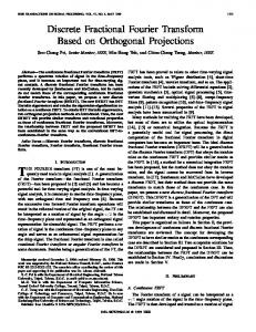
A. Two Types of Factor Graphs We will now consider factor-graph representations for complex-valued functions defined on a finite direct product of finite abelian groups. We will consider functions that factor (either multiplicatively or convolutionally) as a product of local functions, as in the general factorization setting of Section II-C. As in Section II-C, let be a positive integer and let be an index set for the components of the direct . For any nonempty subset of , let product be the subgroup of defined as . A function will be regarded as a function of variables , where variable takes values in group . , and for any , let be Let some nonempty subset of . Suppose a given function defined on factors (either multiplicatively or convolutionally, as in Section II-C) as (7) where local factor is a complex-valued function defined on . For each , it is convenient to define as the subset of that indexes the local factors having as an argument, i.e., . The factorization (7) may be visualized with the aid of the , defined in the following way. The symbol factor graph denotes a bipartite graph with two vertex classes: one class containing variable vertices, each representing one of the vari, and the other class containing function ables , (factor) vertices, each representing one of the local functions , . An edge connects variable vertex with function vertex if and only if appears as an argument of , or, equivalently, . The i.e., if and only if represents the multiplicative factorization graph , and is referred to as a multiplicative factor graph. The graph represents the convolutional factoriza, and is referred to as a convolutional tion instead of when the factor graph. We will write function is clear from context. Example 1: Let , , and groups and factorization

be the direct product of finite abelian , and let , , be three local functions. The generic

is represented by the bipartite graph shown in Fig. 1. Depending on the product operation associated with , this graph can represent either the multiplicative factorization

B. Factor-Graph Duality Using the notation of the previous subsection, let be a direct product group, where is a finite index set. As observed in Section III, the character of is the direct product . If is group denote the direct product a nonempty subset of , we let , and we note that . An arbitrary element of will be denoted as , and an arbitrary will be denoted as . element of Also, as in the previous subsection, let be , an index set for a set of local functions , is a subset of . where, for each Finally, let denote a function product (either multiplication or convolution) and let denote the dual product, i.e., so that and . and , repWe define the pair of factor graphs, resenting the factorizations

respectively. The two factor graphs and are said to be a pair of dual factor graphs. The reader is cautioned to note that is not necessarily the Fourier transform of , since needed scale factors may be missing. However, in light of the multivariate convolution theorem, the following theorem is immediate. Theorem 11: A pair of dual factor graphs represent (up to scale) a Fourier transform pair. C. Convolutional Tanner Graphs As previously defined, let be a finite index set and be a direct product group. In coding theory, one may , , where has consider a set of local codes , where . We consider indicator function two dual ways to define a group code using these local codes. A code may be defined by regarding each local code as a , a valid local constraint in the following sense. For each must codeword of restricted to the positions indexed by , and the code is the set of all words be a codeword of


1643

Fig. 2. (a) Multiplicative Tanner graph for the (7; 4) Hamming code C . (b) Convolutional Tanner graph for the (7; 3) dual Hamming code C . Local functions denoted “+” are indicator functions for a single parity-check code, whereas local functions denoted “=” are indicator functions for a repetition code.

that satisfy all of these local constraints. The local code con, leaving the costrains only the coordinates indexed by free; thus, in effect creates the code ordinates in , and is obtained as (8) By Theorem 2, the indicator function

The following example will clarify this construction. We will consider a binary linear block code of length as a subgroup of the additive group . Example 2: Let , where

, let

and let . Let

is

Thus, the indicator function of code may be represented by a multiplicative factor graph. On the other hand, a(nother) code may be defined by regarding each local code as a generating subgroup , is the identity element of . Then is the where sum of all such subgroups, i.e.,

The matrix has , so we define . , , and We have , indicating the location of the nonzero elements of . is taken as the parity-check matrix of the If Hamming code , then is defined by the single parity-check . Thus, has indicator function equation

(9) By Theorem 2, the scaled indicator function

is

Thus, the scaled indicator function of code may be represented by a convolutional factor graph, which we call a convolutional Tanner graph. In the case of a linear code defined over a finite field , the local codes that give rise to a code may be defined via the is rows of a parity-check matrix or generator matrix for . If an matrix with entries from , then the th row defines , each a subspace of a pair of dual local codes of length , where denotes the set of columns of that have is considered as a paritya nonzero coordinate in row . If check matrix for a code , then is defined by interpreting is a linear the th row as a parity-check equation, so that . In this case, is obtained via (8) code of dimension and hence has a Tanner-graph representation [1]. On the other is considered as a generator matrix for , then hand, if is defined by interpreting the th row as a generator, so that is a linear code of dimension . In this case, is obtained via (9) and hence has a convolutional Tanner-graph representation.

and

has indicator function

which can be represented by the multiplicative Tanner graph in Fig. 2(a). is taken as the generator matrix for the Dually, if dual Hamming code , then is the one-dimensional repetition code with scaled indicator function

Thus

has scaled indicator function

which can be represented by the convolutional Tanner graph in Fig. 2(b). In a more general setting of group codes, let . An -symbol code is obtained in a kernel representation if is the kernel of a group homomorphism mapping into some abelian group . Often, the abelian group itself decomposes as

1644


a direct product , where , and the homomorphism decomposes as a set of homomorphisms such that, for every where

, and is obtained by restricting to the positions indexed by . Then the kernel of each homomorphism forms a local code , with indicator function

and the code is the intersection with indicator function

,

puncturing some coordinates and shortening other coordinates, however, we will not consider such representations here.) The usual purpose of introducing auxiliary (“hidden”) variables is to achieve some simplification of a factor-graph model for a code. For example, auxiliary variables can be introduced to eliminate graph cycles, resulting in a cycle-free representation such as a trellis. Theorem 2 relates indicator functions for with those for the shortened and punctured codes. We have (10) (11)

as before. is obtained in an image Dually, an -symbol code of some homomorphism representation if is the image mapping some finite abelian group into . Often the homomorphism decomposes as a set of homomorphisms , such that for every

Then, the image of each homomorphism code , with scaled indicator function

and the code function

is the sum

forms a local

, with scaled indicator

as before. In essence, a kernel representation works by “cutting away:” starting from the entire configuration space, the code is specified as the intersection of a number of supercodes. On the other hand, an image representation works by “building up:” starting from the zero word, the code is specified as the sum of a number of subcodes. Kernel representations fit naturally with multiplicative factor graphs, while image representations fit naturally with convolutional factor graphs. D. Factor Graphs With Auxiliary Variables Instead of considering the finite abelian group as the direct product , in this subsection, we consider as the direct , where is another index set and product indexes some subgroup of . We will associate each with each index a variable , referred to as an auxiliary variable, taking values from . We will denote the subgroups by and of by . Let be a subgroup of , which we refer to as a “behavior.” We will consider two dual ways to realize a code from is obtained behavior . The punctured code by puncturing the auxiliary variables. The shortened code is obtained by shortening the auxiliary variables. (One might also consider codes obtained from a behavior by

which shows that there is a close (essentially trivial) relationship between a multiplicative factor-graph representation of and multiplicative factor-graph representation of the shortened code , and likewise between a convolutional factor-graph . representation of and the punctured code be a multiplicative factor-graph repSpecifically, let resentation for a given behavior . According to (10), a multiplicative factor graph for the shortened code is obtained factor for every auxiliary variable , by introducing a . Each local factor in the original graph may be replaced with the function obtained by -sampling, i.e., replacing with , where is an index set for the auxiliary variables incident on . As the auxiliary variables then no longer appear as arguments of the and the auxiliary modified functions, edges between variables may be deleted. In effect, the auxiliary variables are connected to Kronecker delta functions and disconnected from the rest of the graph. It is easy to see that the result is a multi. The auxiliary variables and their plicative factor graph for neighbors can, in fact, be deleted from the graph, resulting in a multiplicative factor graph for the shortened code (as conventionally defined). Likewise, there is a trivial relationship between a convolutional factor-graph representation for the punctured code and a convolutional factor-graph representation for . By a procedure similar to that described in the previous paragraph, each is replaced with the function obtained by -avlocal factor eraging, i.e., replacing with and then deleting all edges incident on the auxiliary variables. The auxiliary variables are connected to scaled indicator functions for the corresponding symbol alphabet and disconnected from the rest of the graph. Again, it is easy to see that the result is a convo, and if the auxiliary variables and lutional factor graph for their neighbors are deleted, the result is a convolutional factor graph for the punctured code (as conventionally defined). Unlike the situation described in the previous two paragraphs, there is a nontrivial relationship between a multiplicative factorand a multiplicative factor-graph graph representation for representation for the punctured code . Likewise, there is a nontrivial relationship between a convolutional factor-graph representation for and a convolutional factor-graph represen. In the former case, the multation for the shortened code tiplicative factor graph representing is essentially a (gener-


alized) state realization [5] or TWL graph [2] of , where the auxiliary variables are referred to as state variables. The latter case provides a natural dual representation, which we refer to as a (generalized) syndrome realization for in which the auxiliary variables are referred to as syndrome variables. The rationale for this latter nomenclature should be clear: a given configif and only if the uration in yields a valid codeword of syndrome variables are zero. We will not study syndrome realizations further; however, see [11], [12]. We will conclude this section by stating the following obvious relationship between state and syndrome realizations. Theorem 12: The dual of a generalized state realization for . Likea code is a generalized syndrome realization for wise, the dual of a generalized syndrome realization for is a . generalized state realization for Proof: This follows from Theorems 5 and 11.

1645

Theorem 13: (16) (17) Proof: We have

where the second equality follows from the identity

Likewise V. FACTOR-GRAPH NORMALIZATION In this section, we define notions of normalization for factor graphs, similar to those of Forney [5], and address the connection between factor-graph duality and Forney-graph duality. A. Normalization and Conormalization Let be a function defined on a finite abelian group that factors multiplicatively as for some functions . Similarly, let be a funcfor tion that factors convolutionally as . In these factorizations, the funcsome functions and “interact” (either multiplicatively or convolutions tionally) via the common variable . Let and be “replicas” of the variable , i.e., two different variables defined over the same alphabet as that of . The function

mapping into is a separable function, in which the two factors do not “interact.” However, this function must somehow and . Before expressing this rebe closely related both to lationship, we define the following four functions in . Let

where the last equality follows from the same identity as in the previous case. Similarly, we have

and

(12) (13) (14) (15) and have a multiplicative factorization Clearly, (and, hence, correspond to a multiplicative factor graph), and have a convolutional factorization whereas (and, hence, correspond to a convolutional factor graph). We as the normal extension of , and we refer to refer to as the conormal extension of . Likewise, and are referred to as the normal and conormal extensions of , respectively. and can be obtained The following theorem shows that by averaging the normal or conormal extensions that factor multiplicatively and by sampling the normal or conormal extensions that factor convolutionally.

where the last equality follows by applying the result of the previous case. Theorem 13 generalizes to give normal and conormal extensions for general multiplicative and convolutional products of local functions—as in (7)—in a straightforward (though notationally cumbersome) way. Perhaps the easiest way to describe these extensions is to describe the corresponding factor graphs as follows.

1646

A factor graph for the normal or conormal extension of a function is obtained by introducing an independent “replica” of each variable that appears as an argument of each local factor, thereby obtaining a completely separable product of local functions. This separable product may be interpreted either multiplicatively or convolutionally, as is convenient. The independent factors are then “coupled” by forming the product (either multiplicative or convolutional) with an appropriately defined indicator function, as in Theorem 13. We refer to the factor graph corresponding to the normal (resp., conormal) extension of a function as the normalized (resp., conormalized) factor graph associated with that extension. For example, suppose that the function has a factor graph . The following procedure will create the normalized and conormalized factor graphs associated with the normal and conormal extensions of . Factor-Graph (Co)Normalization Procedure: For every variable vertex having degree : denote the neighbors of . 1) Let 2) Isolate (i.e., delete all edges incident on ) and create independent replica variable vertices having the same alphabet as . 3) Attach replica to local factor . 4) Create a new local code indicator vertex —chosen according to Table I—and connect variable vertex and its replicas to . The resulting factor graph represents the normal or conormal extension of provided that each newly introduced (the local code indicator) is local factor vertex defined appropriately, according to Table I. For example, if the original factor graph is multiplicative then the conormalized (convolutional) factor graph is obtained by selecting

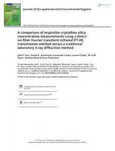
The normalization and conormalization procedures may also be understood as a local graph transformation, in which the local neighborhood of each variable vertex is transformed by substitution of an appropriate tree, as shown for multiplicative graphs in Fig. 3(a) and (b), respectively, and for convolutional factor graphs in Fig. 3(c) and (d), respectively. We remark that, in the normalized or conormalized factor graphs, all variable vertices have degree either one or two; in particular, all introduced replica variable vertices have degree two, and all original variable vertices have degree one. The reader may verify that this normalization procedure (applied to multiplicative factor graphs) is identical to the normalization procedure of Forney [5]. be a direct product group, and let Let and be complex-valued functions on that factor multiplicatively and convolutionally, be the direct product group respectively, as in (7). Let needed to define all replica variables in the (co)normalization as . procedure defined above, and denote an element of The following theorem is the generalization of Theorem 13.


TABLE I LOCAL CODE INDICATOR FUNCTIONS IN (CO)NORMALIZATION OF A FACTOR GRAPH

Theorem 14:

where are the normal and conormal , respectively, and are extensions of the normal and conormal extensions of , respectively. We remark that working with normal or conormal extensions of a given product of local factors gives the system modeler freedom to select the function product type (multiplication or convolution) that is most convenient in any given application. The resulting factor graph is not more complicated than the original one. As we will see in the next section, the Fourier transform of a (co)normal extension is a (co)normal extension of the Fourier transform, and hence, this modeling freedom will extend also to the Fourier transform domain. B. Duality Relationships of Normal Extensions Now we consider the normalization and conormalization of a pair of dual factor graphs and representing and its Fourier transform, a multiplicative product , respectively. Due to the a convolutional product, well-known duality between parity-check codes and repetition codes over any finite abelian group, the new function vertices and the introduced in the normalization procedure on corresponding function vertices introduced in the normalization represent (up to scale) pairs of Fourier procedure on transforms. By the multivariate convolution theorem (Theorem 10), the and are a pair normalized factor graphs of dual factor graphs, representing (up to scale) a Fourier transand , respectively. For the same reason, form pair and are the conormalized factor graphs a pair of dual factor graphs, representing (up to scale) a Fourier and , respectively. transform pair Furthermore, by the Sampling/Averaging Duality Theorem by -averaging of (Theorem 8), the recovery of (summing over the replica variables) corresponds to the reby -sampling of (setting the dual replica covery of variables to zero) in the dual domain. Likewise, the recovery of by -sampling of corresponds to the recovery of by -averaging of in the dual domain. These various relationships are summarized in the commutative diagram of Fig. 4.


1647

Fig. 3. (a) Normalization and (b) conormalization transformations for multiplicative factor graphs; (c) normalization and (d) conormalization transformations for convolutional factor graphs. Local factors designated with an “ ” sign indicate an equality constraint; local factors designated with a “ ” sign indicate that the incident variables must sum to zero. The small circles represent sign inverters.

=

Fig. 4. Commutative diagrams summarizing the relationships between dual factor graphs and the corresponding normalized and conormalized factor graphs. The symbols in each corner are mnemonic, indicating the local code indicator type in each corresponding (co)normal graph.

C. Duality Relationships of Normal Realizations of Codes In the context of coding theory, let the multiplicative factor represent a group code , where the funcgraph tion vertices represent the local codes that intersect to form , as represents in (8). Then the convolutional factor graph the dual code , where the function vertices represent , as in (9). the dual of the local codes that sum to form Let the normalized factor graph and the conormalized factor graph of represent, respectively, two codes and , contained in , represents the product of alphabets corresponding where to all the replica variables. Then the normalized factor graph and the conormalized factor graph of represent, respectively, the dual codes and contained in . By Theorem 2, code may be regarded as the projection of on restricted on restricted to to , or as the cross section of . Dually, code may be regarded as the cross section of on restricted to , or as the projection on restricted to . These relationships, implied by the commutative diagram of Fig. 4, are explicitly summarized in

+

Fig. 5. Commutative diagrams summarizing the relationships between dual, normalized, and conormalized factor-graph representations of codes. (With a slight abuse of notation, instead of using the indicator functions, we use the represented codes as the subscripts of the factor graphs.)

the commutative diagram in Fig. 5. Clearly, and are, respectively, state and syndrome realizations and are, respectively, of . Likewise, . Similar duality relasyndrome and state realizations of tionships are expressed in a similar way by Koetter in [13]. The Forney-graph (or normal-graph) duality of [5] can be understood using this diagram. Suppose that we start with a Tanner graph of code , which is essentially the multiplicative factor graph in Fig. 5. Forney’s normalization procedure on the Tanner graph is identical to the normalization procedure on multiplicative factor graphs in this paper, and the resulting Forney graph is essentially the normalized multiplica. Forney’s dualization procedure on tive factor graph involves dualizing each the normalized factor graph local code represented by the function vertex and inserting a sign inverter between each replica variable vertex and the newly introduced function vertex connecting to it, which gives rise to the dual Forney graph, a multiplicative factor graph iden. Forney-graph duality then states that punctical to and turing the replica (state) variables in code gives rise to the pair of dual codes and —a result that can be obtained by following the arrows in the diagram from

1648


Fig. 6.

Duality relationships between (co)normalized state and syndrome realizations. The pair dual codes of interest are C and C .

TABLE II LOCAL CODE INDICATOR FUNCTIONS FOR AUXILIARY VARIABLES (CO)NORMALIZATION OF A CODE REALIZATION

IN

to and from to . In effect, the Forney-graph duality results are identical to those illustrated in Fig. 5, “skipping over” the convolutional factor graphs. D. Normalizing Realizations With Auxiliary Variables A slight complexity arises when the factor graph prior to normalization does not represent the code of interest, but rather is a state or syndrome realization of the code. In a state realization (as defined in Section IV-D), the represented behavior is punctured on state variables to recover the code of interest. Conormalizing a state realization produces a new realization having variable vertices and their replicas as well as state variables and their replicas. In order to recover the code of interest, this behavior would need to be punctured at the state variables and shortened at the replicas of the state variables and hence this new realization would be neither a valid state realization nor a valid syndrome realization. A similar complication arises when conormalizing a syndrome realization. These complications are easily addressed, however, by treating the (hidden) auxiliary variables slightly differently in the process of normalization than the other variables in the graph (which we refer to as primary variables). This different treatment of primary and auxiliary variables is also required in the construction of Forney graphs: see the separate “symbol replication” and “state replication” procedures in [5, Sec. III-B]. The main difference in the normalization procedure is that, once replicas of an auxiliary variable have been introduced, the original auxiliary variable is deleted, and the local code indicator function is suitably modified, according to Table II. As degree-one auxiliary variables may be absorbed by suitably modifying the neighboring local factor, without loss of generality, we assume that all auxiliary variables appearing in the graph have degree at least two. Following is the factor graph (co)normalization procedure for code realizations with auxiliary variables.

Factor-Graph (Co)Normalization Procedure with Auxiliary Variables: For every primary variable vertex, apply the factor graph (co)normalization procedure described in Section V-A. For every auxiliary variable vertex : denote the neighbors of . 1) Let 2) Isolate (i.e., delete all edges incident on ) and create independent replica variable vertices having the same alphabet as . 3) Attach replica to local factor . — 4) Create a new local code indicator vertex chosen according to Table II—and connect the replicas to . 5) Delete auxiliary variable vertex . The duality relationships between (co)normalized state and syndrome realization are shown in the diagram in Fig. 6. In the representing diagram, the multiplicative factor graph is a state realization of code , and the convolubehavior representing the dual behavior tional factor graph is a syndrome realization of the dual code . The norof and malized factor graphs of represent a pair of normalized dual behaviors, and , respectively, and similarly for and . The code is a projection of and a cross , and likewise, the dual code is a cross section of and a projection of . section of VI. CONCLUDING REMARKS The Fourier transform naturally induces convolution as a function product that is dual to multiplication. Just as multiplication may be defined via periodic extensions of local functions, we have shown that convolution may be defined via impulsive extensions of local functions. We have introduced convolutional factor graphs as a natural graphical representation of the convolutional factorization structure of a multivariate function, just as conventional (multiplicative) factor graphs are a representation of a multiplicative factorization. If a function is represented by one type of factor graph, its Fourier transform is represented by the dual type, with the same underlying graph structure.


Applied to coding theory, this Fourier transform duality yields code duality, as the Fourier transform of an indicator function for a code yields a scaled indicator function for the dual code. The natural dual to a conventional Tanner graph is a convolutional Tanner graph; the former expresses a code as the intersection of supercodes and may be obtained from a parity-check matrix description, and the latter expresses a code as the sum of subcodes and may be obtained from a generator matrix description. In code realizations with auxiliary variables, multiplicative factor graphs give rise to state realizations in which the code of interest is obtained by taking a projection, and convolutional factor graphs give rise to syndrome realizations in which the code of interest is obtained by taking a cross section. By introducing normal and conormal extensions, we have generalized the normalization procedures of Forney [5] to the case of multivariate functions. We show that the elegant Forney-graph duality properties of [5] are easily understood in this framework. An important consequence of working with normalized or conormalized functions is that the choice of function product (multiplication or convolution) essentially becomes arbitrary, and so this choice can be made according to convenience. In either case, the factor graphs corresponding both to and its Fourier transform have the same underlying graph. Function normalization entails no significant expansion of computational effort for local message-passing algorithms; e.g., the sum–product algorithm operates in a normalized multiplicative factor graph with the same complexity as in the original graph. Since the dual graph of a multiplicative graph may also be chosen to be multiplicative, the sum–product algorithm can also be applied in the Fourier transform domain; and in fact, this may result in decreased computational complexity when the Fourier transforms of the local factors are somehow simpler to process than the local factors themselves. (In coding applications, the duals of high-rate local codes are low rate, and may be easier to decode.) These observations lead us to believe that Forney graphs are, for most practical purposes in coding applications, the preferred graphical code representation, as the elegant and useful duality properties that they possess come at no significant increase in the computational complexity of local message-passing algorithms. In applications beyond coding theory, it may be, for the same reasons, that the normalized factor graphs introduced here may also be preferable to other representations.

1649

As convolution and the Fourier transform occur in many areas of science and engineering, the extension of factor graphs to include convolutional factorization and the introduction of factorgraph duality may potentially have applications in some of these areas. A first step in this direction is taken in [14]; see also [15].

ACKNOWLEDGMENT The authors are grateful for the many helpful comments made by the reviewers, R. Koetter, H.-A. Loeliger, and especially, G. D. Forney, Jr. These comments have resulted in a substantially improved paper.

REFERENCES [1] R. M. Tanner, “A recursive approach to low-complexity codes,” IEEE Trans. Inf. Theory, vol. IT-27, no. 5, pp. 533–547, Sep. 1981. [2] N. Wiberg, H.-A. Loeliger, and R. Koetter, “Codes and iterative decoding on general graphs,” Europ. Trans. Telecommun., vol. 6, pp. 513–525, Sep./Oct. 1995. [3] N. Wiberg, “Codes and decoding on general graphs,” Ph.D. dissertation, Linköping Univ., Linköping, Sweden, 1996. [4] F. R. Kschischang, B. J. Frey, and H.-A. Loeliger, “Factor graphs and the sum-product algorithm,” IEEE Trans. Inf. Theory, vol. 47, no. 2, pp. 498–519, Feb. 2001. [5] G. D. Forney Jr., “Codes on graphs: Normal realizations,” IEEE Trans. Inf. Theory, vol. 47, no. 2, pp. 520–548, Feb. 2001. [6] G. D. Forney Jr. and M. D. Trott, “Dynamics of group codes: Dual abelian group codes and systems,” IEEE Trans. Inf. Theory, vol. 50, no. 12, pp. 2935–2965, Dec. 2004. [7] A. Terras, Fourier Analysis on Finite Groups and Applications. Cambridge, U.K.: Cambridge Univ. Press, 1999. [8] E. Hewitt and K. A. Ross, Abstract Harmonic Analysis. New York: Springer-Verlag, 1970. [9] W. Rudin, Fourier Analysis on Groups. New York: Wiley–Interscience, 1962. [10] G. D. Forney Jr., “Transforms and groups,” in Codes, Curves and Signals: Common Threads in Communications, A. Vardy, Ed. New York: Kluwer–Academic, 1998, pp. 79–97. [11] , “Syndrome realizations of linear codes and systems,” in Proc. 2003 IEEE Information Theory Workshop, Paris, France, Mar./Apr. 2003, pp. 214–217. [12] Y. Mao and F. R. Kschischang, “Codes on graphs: State-syndrome realizations,” in Proc. 2003 Canadian Workshop on Information Theory, Waterloo, ON, May 2003, pp. 48–51. [13] R. Koetter, “On the representation of codes in Forney graphs,” in Codes, Graphs and Systems, R. E. Blahut and R. Koetter, Eds. New York: Kluwer–Academic, 2002. [14] Y. Mao, F. R. Kschischang, and B. J. Frey, “Convolutional factor graphs as probabilistic models,” in Proc. Uncertainty in Artificial Intelligence (UAI), Banff, AB, Jul. 2004, pp. 374–381. [15] Y. Mao, “A duality theory for factor graphs,” Ph.D. dissertation, Univ. Toronto, Dep. Elec. Comput. Eng., Toronto, ON, Canada, 2003.