patches, randomly sampled from the two face images, and scoring the patches (or features) by their mutual distances. In order to deal with the multi-scale nature ...
On Finding Differences Between Faces Manuele Bicego1 , Enrico Grosso1, and Massimo Tistarelli2 2
1 DEIR - University of Sassari, via Sardegna 58 - 07100 Sassari - Italy DAP - University of Sassari, piazza Duomo 6 - 07041 Alghero (SS) - Italy
Abstract. This paper presents a novel approach for extracting characteristic parts of a face. Rather than finding a priori specified features such as nose, eyes, mouth or others, the proposed approach is aimed at extracting from a face the most distinguishing or dissimilar parts with respect to another given face, i.e. at “finding differences” between faces. This is accomplished by feeding a binary classifier by a set of image patches, randomly sampled from the two face images, and scoring the patches (or features) by their mutual distances. In order to deal with the multi-scale nature of natural facial features, a local space-variant sampling has been adopted.
1
Introduction
Automatic face analysis is an active research area, whose interest has grown in the last years, for both scientific and practical reasons: on one side, the problem is still open, and surely represents a challenge for Pattern Recognition and Computer Vision scientists; on the other, the stringent security requirements derived from terroristic attacks have driven the research to the study and development of working systems, able to increase the total security level in industrial and social environments. One of the most challenging and interesting issue in automatic facial analysis is the detection of the “facial features”, intended as characteristic parts of the face. As suggested by psychological studies, many face recognition systems are based on the analysis of facial features, often added to an holistic image analysis. The facial features can be either extracted from the image and explicitly used to form a face representation, or implicitly recovered and used such as in the PCA/LDA decomposition or by applying a specific classifier. Several approaches have been proposed for the extraction of the facial features ([1–5], to cite a few). In general terms, all feature extraction methods are devoted to the detection of a priori specified features or gray level patterns such as the nose, eyes, mouth, eyebrows or other, non anatomically referenced, fiducial points. Nevertheless, for face recognition and authentication, it is necessary to also consider additional features, in particular those features that really characterize a given face. In other words, in order to distinguish the face of subject “A” from the face of subject “B”, it is necessary to extract from the face image of subject “A” all features that are significantly different or even not present in face “B”, rather than extract standard patterns. T. Kanade, A. Jain, and N.K. Ratha (Eds.): AVBPA 2005, LNCS 3546, pp. 329–338, 2005. c Springer-Verlag Berlin Heidelberg 2005 �
330
Manuele Bicego, Enrico Grosso, and Massimo Tistarelli
This paper presents a novel approach towards this direction, aiming at “finding differences” between faces. This is accomplished by extracting from one face image the most distinguishing or dissimilar areas with respect to another face image, or to a population of faces.
2
Finding Distinguishing Patterns
The amount of distinctive information in a subject’s face is not uniformly distributed within its face image. Consider, as an example, the amount of information conveyed by the image of an eye or a chin (both sampled at the same resolution). For this reason, the performance of any classifier is greatly influenced by the uniqueness or degree of similarity of the features used, within the given population of samples. On one side, by selecting non-distinctive image areas increases the required processing resources, on the other side, non-distinctive features may drift or bias the classifier’s response. This assert is also in accordance with the mechanisms found in the human visual system. Neurophysiological studies from impaired people demonstrated that the face recognition process is heavily supported by a series of ocular saccades, performed to locate and process the most distinctive areas within a face [6–10]. In principle, this feature selection process can be performed by extracting the areas, within a given subject’s face image, which are most dissimilar from the same areas in a “general” face. In practice, it is very difficult to define the appearance of a “general face”. This is an abstract concept, definitely present in the human visual system, but very difficult to replicate in a computer system. A more viable and practical solution is to determine the face image areas which mostly differ from any other face image. This can be performed by feeding a binary classifier with a set of image patches, randomly sampled from two face images, and scoring the patches (or features) by their mutual distances, computed by the classifier. The resulting most distant features, in the “face space”, have the highest probability of being the most distinctive face areas for the given subjects. In more detail, the proposed algorithm extracts, from two face images, a set of sub-images centered at random points within the face image. The sampling process is driven to cover most of the face area1 . The extracted image patches constitute two data sets of location-independent features, each one characterizing one of the two faces. A binary Support Vector Machine (SVM) [16, 17] is trained to distinguish between patches of the two faces: the computed support vectors define a hyperplane separating the patches belonging to the two faces. Based on the distribution of the image patches projected on the classifier’s space, it is possible to draw several conclusions. If the patch projection “lies” very close to the computed hyperplane (or on the opposite side of the hyperplane), it means 1
A similar image sampling model has been already used in other applications such as image classification (the so called patch-based classification [11–14]) or image characterization (the epitomic analysis proposed by Joijc and Frey in [15])
On Finding Differences Between Faces
331
that the classifier is not able to use the feature for classification purposes (or it may lead to a misclassification). On the other hand, if the patch projection is well located on the subject’s side of the hyperplane and is very far from the separating hyperplane, then the patch clearly belongs to the given set (i.e. to that face) and it is quite different from the patches extracted from the second face. According to this intuition, the degree of distinctiveness of each face patch can be weighted according to the distance from the trained hyperplane. Since the classifier has been trained to separate patches of the first face from patches of the second face, it is straightforward to observe that the most important differences between the two faces are encoded in the patches far apart from the separating hyperplane (i.e. the patches with the highest weights). In this framework the scale of the analysis is obviously driven by the size of the extracted image patches. By extracting large patches only macro differences are determined, loosing details, while by reducing the size of the patches only very local features are extracted, loosing contextual information. Both kinds of information are important for face recognition. A possible solution is to perform a multi scale analysis, by repeating the classification procedure with patches at different sizes, and then fusing the determined differences. The drawback is that each analysis is blind, because no information derived from other scales could be used. Moreover, repeating this process for several scales is computationally very expensive. A possible, and more economic, alternative to a multi-scale classification, is to extract “multi-scale” patches, i.e. image patches which encode information at different resolution levels. This solution can be implemented by sampling the image patches with a log-polar mapping [18]. This mapping resembles the distribution of the ganglion cells in the human retina, where the sampling resolution is higner in the center (fovea) and decreases toward the periphery. By this resampling of the face image, each patch contains both low scale (high resolution) and contextual (low resolution) information. The proposed approach for the selection of facial features consists of three steps: 1. two distinct and geometrically disjoint sets of patches are extracted, at random positions, from the two face images; 2. a SVM classifier is trained to define an hyperplane separating the two sets of patches; 3. for each of the two faces, the face patches are ranked according to the distances from the computed hyperplane. The processes involved by each step are detailed in the remainder of the paper. 2.1
Multi-scale Face Sampling
A number of patches are sampled from the original face image, centered at random points. The randomness in the selection of the patch center assures that
332
Manuele Bicego, Enrico Grosso, and Massimo Tistarelli
the entire face is analyzed, without any preferred side or direction. Moreover, a random sampling enforces a blind analysis without the need for a priori alignment between the faces. The face image is re-sampled at each selected random point following a logpolar law [18]. The resulting patches represent a local space-variant remapping of the face image, centered at the selected point. The analytical formulation of the log-polar mapping describes the mapping that occurs between the retina (retinal plane (x, y)) and the visual cortex (log-polar or cortical plane (log(ρ), θ)). The derived logarithmic-polar law, taking into account the linear increment in size of the receptive fields, from the central region (fovea) towards the periphery, is described by the diagram in figure 1(a).
(a)
(b)
Fig. 1. (a) Retino-cortical log-polar transformation. (b) Arrangement of the receptive fields in the retinal model
The log-polar transformation applied is the same described in [18] which differs from the models proposed in [19, 20]. The parameters required to define the log-polar sampling are: the number of receptive fields per eccentricity (Na ) and the radial and angular overlap of neighboring receptive fields (Or and Oa ). For each receptive field, located at eccentricity ρi and with radius Si , the angular overlap factor is defined by K0 = Sρii . The amount of overlapping is strictly related to the number of receptive fields per eccentricity Na . In particular if K0 = Nπa all receptive fields are disjoint. The radial overlap is determined by: K1 =
Si ρi = . Si−1 ρi−1
The two overlap parameters K0 and K1 are not independent, in fact: K1 =
ρi 1 + K0 = . ρi−1 1 − K0
As for the angular overlap, the radial overlap is not null only if: K1