On fitting dielectric spectra using artificial neural networks - CiteSeerX

Bioelectrochemistry and Bioenergetics, 28 (1992) 425-434 A section of J. Electroanal. Chem., and constituting Vol. 343 (1992) Elsevier Sequoia S.A., Lausanne

JEC BB 01527

On fitting dielectric spectra using artificial neural networks Douglas B. Kell

and Christopher L. Davey

Department of Biological Sciences, University College of Wales, Aberystnyth, Dyfed SY23 3DA (UK) (Received 20 September 1991; in revised form 30 December 1991)

Abstract

In biological dielectric spectroscopy, where dispersions are substantially broader than that expected from a purely Debye-like process, it is not always possible, because of technical limitations, to obtain data over a wide enough range of frequencies to encompass the entire dispersion(s) of interest. Similarly, because of the breadth of the dispersions, it is common to seek to characterize the dielectric behaviour of interest by means of the Cole-Cole function. Whilst it is possible to fit dielectric data to this equation using appropriate non-linear least-squares methods, these methods are computationally rather demanding, and must be performed iteratively for each set of data. We show here, for the first time, that it is possible to train an artificial neural network to learn to extract the parameters of the Cole-Cole equation from small sets of dielectric data (permittivities measured at various frequencies) which can thus give an essential instantaneous output of the limiting permittivities at frequencies that are both high and low with respect to the characteristic frequency.

INTRODUCTION

In the dielectric spectroscopy of biological and other systems, it is usual to find areas of strong frequency dependence, known as dielectric dispersions, in which the measured permittivity decreases with increasing frequency, with a shape (when the frequency is plotted logarithmically) approximating an inverse sigmoid [I-121. To characterize the behaviour of the system of interest quantitatively, one fits the measurements (permittivity and conductivity at different frequencies) to an appropriate equation, that proposed by Cole and Cole [I31 being perhaps the most 'T o whom correspondence should be addressed. 0302-4598/92/$05.00 Q 1992 - Elsevier Sequoia S.A. All rights resewed

popular in biological work. The Cole-Cole equation is a modification of the Debye [14] formulation of molecular dielectric behaviour which contains, in addition to the dielectric increment A E , the characteristic frequency f, and the high-frequency permittivity E,,, an empirical parameter, the Cole-Cole a , which can be used to describe (if not to explain) the fact that real dielectric spectra are much broader than those due to a simple Debye-like dispersion. Whilst the Cole-Cole cw has no theoretical justification (although it is widely interpreted in terms of a distribution of relaxation times), Schwan [I51 showed that a great many types of relaxation-time distribution could accurately fit the Cole-Cole function. In addition, the Cole-Cole function permits one to extract the parameters describing an entire dielectric dispersion, even if, for technical reasons, one cannot measure over the whole frequency range across which it occurs. For these and other reasons, the Cole-Cole formulation remains very popular as a means of characterizing the dielectric properties of biological systems. We have shown that the radio-frequency dielectric properties of biological cells at one or two appropriate frequencies can be used as a rapid (on-line) method for measuring levels of cellular biomass in fermentors and elsewhere, and for this purpose we have constructed a high-resolution dielectric spectrometer, capable of measuring in the range 0.2-10 MHz [16-201. The method relies upon the fact that the P-dielectric dispersion exhibited by all biological cells is dominated by the charging of their plasma membrane(s), and that intact biological cells, but nothing else likely to be found in a fermentor, possess relatively non-conducting plasma membranes [16]. However, this approach requires that (i) at least one of the frequencies of measurement is low with respect to fc, and (ii) the fc does not change appreciably during the fermentation of interest. The fc of the /3 dielectric dispersion depends upon both the internal and external conductivity [15], and whilst the former is likely to be a relatively constant property (at least for cells in a given medium) the latter may well change significantly [21]. One way round the above problem would be to take measurements at a number of frequencies and fit the data to the Cole-Cole equation, thereby obtaining the dielectric increment which is what truly reflects the biomass present [16-201. Methods for fitting dielectric data are usually based on non-linear least-squares algorithms [1,22], and we ourselves (see later) have found that the popular Levenberg-Marquardt algorithm [23,24] provides excellent fits to real dielectric spectra. However, these methods are computationally rather intensive, and for the fermentor example would have to be carried out for every data set at every time point. Artificial neural networks (ANNs) consists of highly interconnected parallelprocessing elements known as nodes, which are arranged in layers representing a set of inputs, one or more so-called hidden layers and a set of outputs. Each node acts to sum its own inputs (which are the outputs of the elements of previous layers), and the sum is passed through a transfer function (which must be continuously differentiable and is normally non-linear) to the element(s) in the next layer. In the classical version, the transfer function is sigmoidal (via the

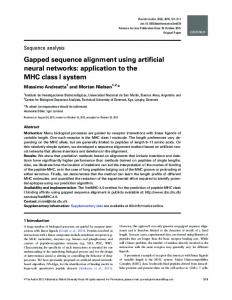
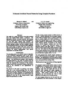
INPUT LAYER

HIDDEN LAYEll(s)

OUTPUT LAYER

Fig. 1. The principle of a classical feedfonvard neural network. (A) The construction of a 4-2-2 neural network in which inputs and outputs are connected to each other via one or more hidden layers. Layers other than the input layer may also be connected to a bias. In the architecture shown, adjacent layers of the network are fully interconnected, although other architectures are possible. (B) Information processing by a neuron. An individual neuron sums its inputs from neurons in the previous layer, transforms them via a transfer function, and outputs them to the next neurons to which it is connected.

exponential term) and is normalized between 0 and 1. The output oj of node j is given by

where

In eqn. (2), 6, is a bias term, oi is the output from the ith node of the previous layer, wi, represents the so-called weight or strength between node i and node j and y is known as the gain. Other popular functions include the sinh, tanh and sine functions, and the general principles of such networks are illustrated in Fig. 1. It is possible to train such networks by initially setting the weights and biases to small random values, presenting the networks with known inputs and outputs, and comparing the output of the net with the "true" (known) outputs. By adjusting the weights using information based on the difference (the error e,) between the output of the net and the true values, a principle known as the back-propagation of error (or, more simply and more commonly, back-propagation or back-prop), it is therefore possible to train the network accurately to deliver a desired output when

presented with a novel (previously unseen) input [25]. This process is repeated from the output through each hidden layer to the input. The actual weight updates for this so-called delta rule are

where LR and M are user-defined values of the so-called learning rate and momentum respectively. In this way, weights are changed according to both the error and the input to the connection of interest. Training can be continued until a defined root mean square error (between the "true" outputs of the training set and the outputs of the network) is obtained, or simply for a fixed number of presentations of the training set. The great interest in ANNs has therefore been aroused by their ability to act as pattern recognition or signal processing elements, among other applications, and ANNs are the subject of a number of books [25-351. This is not the place to review in detail what is a very substantial literature, but the following outline comments are in order. First, it has been shown that (given sufficient time) an appropriately trained network with sufficient nodes can simulate any function to an arbitrary degree of accuracy [36]. Second, whilst back-propagation methods are nowadays considered to be computationally rather inefficient, and many other possible algorithms and architectures exist [37-421, they remain the most popular methods and their behaviour is reasonably well understood. Third, although the training of a network may be a lengthy procedure, once trained the network processes the input into the output virtually instantaneously. Fourth, it is widely believed that, owing to the parallel distributed processing that they effect, the networks are robust with respect to both noise in the inputs and "damage" to the neurons [43,44]. Finally, for our present purposes, it is pertinent to note that ANNs have been used with success in the analysis of nuclear magnetic resonance (NMR) spectra [45] and fluorescence spectra [461, and in chromatography [471. The question therefore arose as to whether it might be possible to train an ANN using simulated dielectric data (permittivity values at a number of fixed frequencies) as the inputs and the parameters of the Cole-Cole equation that had generated the data as the outputs, and thereby teach the network to give (say) the dielectric increment of a dispersion when presented with a set of dielectric data that have (realistically) variable values of E,, f, and a. In the present work, we show that this is indeed the case. METHODS

All simulations and networks were run on a Viglen Vig I11 80386-based PC-compatible microcomputer, incorporating an 80387 coprocessor. Simulations were run using programs written in-house in Microsoft QuickBasic (Version 4.5).

The neural networks were produced and run using the Neural Works Explorer package (Scientific Computers, Burgess Hill, UK), whilst non-linear least-squares fitting (according to the Levenberg-Marquardt algorithm) routines were performed and displayed, together with other plots, using GraFit version 2 (Erithacus Software, Staines, UK).

RESULTS AND DISCUSSION

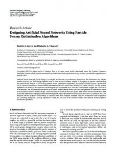
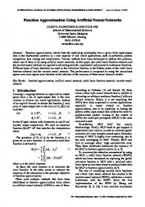
Figure 2 gives an illustration of the present problem of interest. Figure 2(A) simulates the dielectric properties of a system in which AE, E , and a are fixed (at values of 500, 100 and 0.1 respectively), whilst f, is varied from 0.3 to 0.7 MHz. The effect on the permittivity measured at 0.3 MHz, a typical frequency of measurement in this application [16-201, is striking, with the apparent permittivity (which one might take as a measure of the biomass) varying from 350 to nearly 500. As mentioned, the dielectric increment, which is the true measure of biomass, is constant under these conditions. Similar curves (in which the permittivity at 0.3 MHz varies under conditions of constant AE) were easily generated as a function of changes in E, (which would occur due to changes in the gas hold-up of a culture) or in a (caused, for instance, by changes in the morphology or degree of heterogeneity of a culture), but are not displayed herein.

Frequency /Hz

Characteristic 1"requcncy /kHz

Fig. 2. Variation of the apparent permittivity at a fixed frequency for a dielectric dispersion of constant dielectric increment, high-frequency permittivity and Cole-Cole a. (A) Frequency dependence of the permittivity. Simulations of eqn. (4) were performed using the following values for the parameters: ch = 100, AE = 500 and a = 0.1. The characteristic frequency f, was varied in steps of 0.1 MHz between 0.3 and 0.7 MHz as indicated. (B) Dependence of the permittivity at 0.3 MHz on the characteristic frequency. Parameters were as in (A).

We therefore created various data sets for training an ANN to fit dielectric spectra to the Cole-Cole equation. The Cole-Cole equation [13] describing the variation of (the real part of the) permittivity with frequency is E f = E,,

+

AE [l + ( f/fc)

l-"

sin (arr/2)]

1 + 2( f/fC)lwa sin ( a ~ / 2 )+ ( f/fc)2-2a

This equation was used to generate 500 sets of data for E at ten different frequencies, logarithmically spaced in the range 0.2-10 MHz, using randomized values of the parameters in the range 0 < AE < 3000, 10'