On Information Theory and Unsupervised Neural Networks

On Information Theory and Unsupervised Neural Networks

Mark D. Plumbley CUED/F-INFENG/TR.78 13th August 1991

Summary

In recent years connectionist models, or neural networks, have been used with some success in problems related to sensory perception, such as speech recognition and image processing. As these problems become more complex, they require larger networks, and this typically leads to very slow training times. Work on these has primarily involved the use of supervised models, networks with a `teacher' which indicates the desired output. If it were possible to use unsupervised models in the early stages of systems to help with the solutions to these sensory problems, it might be possible to approach larger and more complex problems than are currently attempted. We may also gain more insight into the representation of sensory data used in such sensory systems, and this may also help with our understanding of biological sensory systems. In contrast to supervised models, unsupervised models are not provided with any teacher input to guide them as to what they should `learn' to perform. In this thesis, an information-theoretic approach to this problem is explored: in particular, the principle that an unsupervised model should adjust itself to minimise the information loss, while in some way producing a simpli ed representation of its input data as output. Initially, general concepts about information theory, entropy and mutual information are reviewed, and some systems which use other information-theoretic principles are described. The concept of information loss and some of its properties are introduced, and this concept is related to Linsker's Ìnfomax' principle. The information loss across supervised learning systems is brie y considered, and various conditions are described for a close match between minimisation of information loss and minimisation of various distortion measures. Next information loss across a simple linear network with one layer of processing units is considered. In order to progress, an assumption must be made concerning the noise in the system instead. With the noise on the input to the network dominant, a network which performs a type of principal component analysis is optimal. A common framework for various neural network algorithms which nd principal components of their input data is derived, these are shown to be equivalent in an information transmission sense. The case of signi cant output noise for position and time-invariant signals is considered. Given a power cost constraint in our system, the form of the optimumlinear lter required to minimisethe information loss under this constraint is analysed. This lter changes in a non-trivial manner with varying noise levels, mirroring the way that the response of biological retinal systems changes as the background light level changes. When the output noise is dominant, the optimumcon guration can be found by using anti-Hebbian algorithms to decorrelate the outputs. Various forms of networks of this type are considered, and an algorithm for a novel Skew-Symmetric Network which employs inhibitory interneurons is derived, which suggests a possible rôle for cortical back-projections. In conclusion, directions for further work are suggested, including the expansion of this analysis for systems with various non-linearities; and general problems of representation of sensory information are discussed.

i

Acknowledgements

There are so many people whose ideas and comments have found their way into this thesis in some way or another, that it would be impossible to name them all. The Speech, Vision and Robotics Group, past and present, must get a special mention, including my supervisor Frank Fallside, and Tony Robinson, Patrick Gosling, Niranjan, Richard Prager, Dave Rainton, Tim (`Large Waster') Marsland, Mike (`Small Waster') Chong, Visakan and Maha Kadirkamanathan, Steve Young, Ron Daniel, and many, many more. Particular thanks to Patrick and Niranjan for proof-reading, and also to Mavis Barber for helping to keep everything running smoothly. Finally, my thanks to Penny, whose support and occasional reminders meant that this thesis did get written|eventually.

This report is adapted from my Ph.D. thesis of 30th May 1991 entitled Àn InformationTheoretic Approach to Unsupervised Connectionist Models'. It covers part of my work between January 1987 and May 1991 at Cambridge University Engineering Department on Information Theory and Neural Networks. Between January 1987 and December 1989 I was nancially supported by an award from the U.K. Science and Engineering Research Council. Since January 1990 I have been employed at CUED as a Research Associate on the application of Genetic Algorithms to Neural Networks.

ii

Contents 1 Introduction

1

2 Information Theory and Perceptual Processing

3

2.1 A Brief Introduction to Information Theory : : : : : : : : : : : : : : : : : : : : : : 2.1.1 General Concepts : : : : : : : : : : : : : : : : : : : : : : : : : : : : : : : : : 2.1.2 Random Variables : : : : : : : : : : : : : : : : : : : : : : : : : : : : : : : : 2.1.3 Entropy : : : : : : : : : : : : : : : : : : : : : : : : : : : : : : : : : : : : : : 2.1.4 Mutual Information : : : : : : : : : : : : : : : : : : : : : : : : : : : : : : : 2.1.5 I-Divergence : : : : : : : : : : : : : : : : : : : : : : : : : : : : : : : : : : : 2.2 Information Theory in Psychology : : : : : : : : : : : : : : : : : : : : : : : : : : : 2.3 Unsupervised Neural Networks : : : : : : : : : : : : : : : : : : : : : : : : : : : : : 2.3.1 Cross-Entropy Maximisation: \G-Max" : : : : : : : : : : : : : : : : : : : : 2.3.2 Maximising of Mutual Information between Output Units: \I-Max" : : : : 2.3.3 Minimising Information Loss : : : : : : : : : : : : : : : : : : : : : : : : : : 2.4 Information Loss across a Network : : : : : : : : : : : : : : : : : : : : : : : : : : : 2.4.1 Properties of Information Loss : : : : : : : : : : : : : : : : : : : : : : : : : 2.4.2 Minimisation of Information Loss by Supervised Learning : : : : : : : : : : 2.4.3 Minimising Information Loss by Minimising Distortion : : : : : : : : : : : : 2.4.4 Information Loss and Infomax : : : : : : : : : : : : : : : : : : : : : : : : : 2.4.5 Applying Information Loss : : : : : : : : : : : : : : : : : : : : : : : : : : :

3 3 4 5 6 7 8 9 9 10 12 13 13 14 15 19 22

3 Principal Component Analysis

23

4 Filtering for Optimal Information Capacity

38

3.1 Transforming for Principal Components : : : : : : : : : : : : : : : : : : : : : : : : 3.1.1 Properties of the KLT : : : : : : : : : : : : : : : : : : : : : : : : : : : : : : 3.1.2 The Projection Induced by WM : : : : : : : : : : : : : : : : : : : : : : : : : 3.1.3 Problems With PCA : : : : : : : : : : : : : : : : : : : : : : : : : : : : : : : 3.2 Information Lost by Principal Components Analysis : : : : : : : : : : : : : : : : : 3.2.1 An Upper Bound on Information Loss : : : : : : : : : : : : : : : : : : : : : 3.2.2 Implications for the Scaling Problem : : : : : : : : : : : : : : : : : : : : : : 3.3 Neural Network Algorithms for PCA : : : : : : : : : : : : : : : : : : : : : : : : : : 3.3.1 The Algorithms : : : : : : : : : : : : : : : : : : : : : : : : : : : : : : : : : : 3.3.2 A Common Framework : : : : : : : : : : : : : : : : : : : : : : : : : : : : : 3.3.3 Orthonormalising the Weights : : : : : : : : : : : : : : : : : : : : : : : : : : 3.3.4 Discussion : : : : : : : : : : : : : : : : : : : : : : : : : : : : : : : : : : : : : 4.1 Whitening Filters : : : : : : : : : : : : : : : : : : : : : : : : : : : : : : : : : : : : : 4.2 Information Transmission with Receptor Noise : : : : : : : : : : : : : : : : : : : : 4.2.1 Bounding curves : : : : : : : : : : : : : : : : : : : : : : : : : : : : : : : : : 4.2.2 Typical Filter : : : : : : : : : : : : : : : : : : : : : : : : : : : : : : : : : : : 4.3 Information Loss and Redundancy Reduction : : : : : : : : : : : : : : : : : : : : : 4.3.1 Equivalence with Constrained Information Loss : : : : : : : : : : : : : : : : 4.3.2 Results of Atick and Redlich : : : : : : : : : : : : : : : : : : : : : : : : : : iii

23 23 25 25 26 28 29 29 30 31 36 37 39 41 42 46 46 47 48

4.4 Discussion : : : : : : : : : : : : : : : : : : : : : : : : : : : : : : : : : : : : : : : : : 48 5 Anti-Hebbian Learning

49

6 Conclusions

68

5.1 5.2 5.3 5.4 5.5

Outline : : : : : : : : : : : : : : : : : : : : : : : : : : : : : : : : : : : : : : : : : : 5.1.1 Small Output Noise : : : : : : : : : : : : : : : : : : : : : : : : : : : : : : : Forward Linear Prediction : : : : : : : : : : : : : : : : : : : : : : : : : : : : : : : : Recurrent Linear Prediction : : : : : : : : : : : : : : : : : : : : : : : : : : : : : : : Symmetrical Recurrent Anti-Hebb Learning : : : : : : : : : : : : : : : : : : : : : : 5.4.1 A Two Dimensional Example : : : : : : : : : : : : : : : : : : : : : : : : : : Skew-Symmetric Interneurons : : : : : : : : : : : : : : : : : : : : : : : : : : : : : : 5.5.1 Properties at Convergence : : : : : : : : : : : : : : : : : : : : : : : : : : : : 5.5.2 Another View of the Skew-Symmetric Network : : : : : : : : : : : : : : : : 5.5.3 Example Simulations : : : : : : : : : : : : : : : : : : : : : : : : : : : : : : : 5.6 Discussion : : : : : : : : : : : : : : : : : : : : : : : : : : : : : : : : : : : : : : : : : 6.1 General Conclusions : : : : : : : : : : : : : : : : : : : : : : : : : : : : : : : : : : : 6.2 Further Work : : : : : : : : : : : : : : : : : : : : : : : : : : : : : : : : : : : : : : : 6.2.1 Non-linear pre-processing : : : : : : : : : : : : : : : : : : : : : : : : : : : : 6.2.2 Winner-Take-All: The ultimate non-linearity : : : : : : : : : : : : : : : : : 6.2.3 Generalising Winner-Take-All : : : : : : : : : : : : : : : : : : : : : : : : : :

iv

49 50 51 52 54 57 59 62 62 63 65 68 69 69 70 73

List of Symbols

X, Y , : : : Pr() pX (x), PX (x), p(x), q (x),: : : E (X ) H (X ), H (Q) H (X; Y ), H (X jY ) I (X ; Y ) DI (p; q ) p , p G X I , I (X; Y )

X, Y x, y fW () N, M DMSE ( ; Y ) tr(M ) N (; 2 )

Random variables (r.v.) Probability of event Probability density, distribution (p.d.) Expected value of X Entropy of r.v. X , p.d. Q Joint, conditional entropy Mutual information between X and Y I-divergence from p to q Mean and variance of p `G-max' cross-entropy measure Covariance matrix of X Information loss Feature r.v. (original patterns) Network input, output r.v.s Network input, output vectors Network function Number of inputs, outputs Mean Squared Error distortion Trace of matrix M Normal p.d. Component-wise cross-entropy distortion DCE SLF True cross-entropy distortion DCE MMI Cost function J , JW Lagrange multipliers , Dirac delta function () Forward weight matrix WT Orthogonal projection P Moore-Penrose Pseudo-inverse W+ X Additive noise on X (r.v.) Value of W at step n Wn Update factor n diag(M ) Diagonalisation of matrix M UT(M ), UT+(M ) Upper, strictly upper triangularisation Forgetting factor Wn n vec(M ) Vectorisation of matrix M Matrix Frobenius norm k kF v

2.1.2 2.1.2 2.1.2 2.1.2 2.1.3 2.1.3 2.1.4 2.1.5 2.1.5 2.3.1 2.3.2 2.3.3, 2.4.1 2.3.3 2.4.1 2.4.1 2.4.2 2.4.3 2.4.3, 3.1.1 2.4.3 2.4.3 2.4.3 2.4.3 2.4.4 2.4.4 2.4.4 3.1 3.1.2 3.1.2 3.2 3.3.1 3.3.1 3.3.1 3.3.1 3.3.2 3.3.2 3.3.4

vi

LIST OF SYMBOLS

Frequency ( ), ( ) Receptor, channel signal power density ( ), ( ) Receptor, channel noise power density Bandwidth limit () Information capacity density () Filter power spectral gain , Total channel capacity, power cost , Receptor, channel signal-to-noise ratio Redundancy Capacity Output r.v. after additional noise Inhibitory weight matrix V IN N N identity matrix Power cost for weight matrix W SW Number of epochs k Interneurons response vector, r.v. z, Z Forward excitation weight matrix UT Target vector t f Sr f Sc f Nr f N c f B C f Gf CT PT Rr R c R C

4.1 4.1 4.1 4.1 4.1 4.1 4.1 4.2 4.3 4.3 5.1 5.2 5.2 5.2 5.4.1 5.5 5.5.2 6.2.2

Chapter 1 Introduction Perception is easy. It must be easy|we do it all the time, and hardly notice: it is eortless and unconscious. Unfortunately, building machines which perceive is more tricky. The problems of speech recognition and image recognition by machine have been the object of much research eort over many years, and both are still dicult problems. One avenue of research in recent years is the eld of Connectionist Models, or Arti cial Neural Networks (sometimes simply Neural Networks). By taking ideas from the way biological neural systems are thought to operate, it is hoped that arti cial systems may be built which are able to take advantage of some of the properties of biological systems. The operation of these arti cial sensory systems may also help to explain the behaviour of real biological systems. However, while it is possible to analyse biological systems at a very low level of up to a few neurons, and at a high level, in terms of the function of whole areas of the brain, our understanding of the intermediate levels in rather limited. In order to proceed, we must either wait for our understanding of biological perceptual systems to progress to these intermediate levels of organisation, or we must theorise|make a `guess' at some general principle which may be involved. The principle we employ in this thesis is an information-theoretic one. The idea is simple: since a sensory system processes information about the outside world, to be used by the organism or machine to aid its ability to operate in the world, we should be able to quantify the amount of information so processed in terms of Shannon's Ìnformation Theory' [Shannon, 1948], well known to communications engineers. Given constraints in our system such as limited numbers of neurons, limited energy, and so on, the sensory system should attempt to retain as much information as possible: a principle of constrained minimisation of information loss. The idea behind such a principle is not new: one of the earliest proponents was Attneave [1954], who originally suggested that information theory was important in perception a few years after Shannon's original work. He suggested, for example, that information in an image was concentrated around the edges and corners, since these are areas of greatest uncertainty in the image. Observing these edges and corners thus gains us more information that other areas of an image. More recently, Linsker [1988b] suggested an Ìnfomax' principle, that a perceptual system should organise itself to transmit maximum information. This is virtually identical to the minimisation of information loss across the system, although certain possibly important dierences arise when considering the details. In particular, if a perceptual system can only measure, say, second order statistics of the data that it observes (i.e. covariance), the Ìnfomax' principle will nd an upper bound for the transmitted information, while the minimum information loss approach will nd an upper bound for the loss of information|a damage limitation approach. Despite these details, the implications of both principles are similar, and give a data-driven approach to the problem of developing arti cial sensory systems. Although there may be constraints and costs associated with the operation of a sensory system, the prime concern should be the transmission of information: changing its representation to a more convenient form for later 1

2

CHAPTER 1.

INTRODUCTION

processing, while minimising the information lost in the process. Using this approach, we hope that we may gain a better understanding of the problem of the design of sensory systems, both biological and arti cial. Organisation

In this thesis, we explore the principle of minimisation of information loss, and its consequences; initially for supervised learning systems (systems with a teacher), but primarily for unsupervised learning systems. Although mainly concentrating on analysis of linear unsupervised systems, albeit with non-linear learning algorithms, towards the end we explore some of the problems of non-linear systems, especially with regard to the popular `Winner-Take-All' approach. In chapter 2 we review some concepts from information theory, and introduce the idea of information loss across a network as a measure of network performance. We consider the implications of this for supervised learning systems, and compare it with Linsker's Ìnfomax' criterion. In chapter 3 we examine Hebbian neural network algorithms which perform a principal components analysis (PCA) of their input data. We nd that many of these algorithms can be combined in a common framework, and they all perform a direct minimisation of information loss over time, if the only noise in the system is on the inputs to the network. In chapter 4 we consider systems with noise on both the inputs and the outputs. If we are dealing with signals such as speech or image signal whose statistics are time- or space-invariant, we can minimise the information loss in the frequency domain. We derive an analytic expression for the optimal lter which minimises information loss for a given power cost, and show how the form of this lter changes with relative input and output noise levels. Chapter 5 considers anti-Hebbian learning algorithms, for minimising information loss for a given power cost when noise on the output of the network is dominant. We need no space-invariant assumptions in this case. We show that some anti-Hebbian learning algorithms minimise power cost while attempting to keep the information loss identical. For other architectures, we derive anti-Hebbian learning algorithms which directly decrease the constrained cost function over time. One of these leads to an architecture with inhibitory interneurons, and a simple anti-Hebbian learning algorithm with a weight decay function. Finally, we look at the requirements for, and problems associated with non-linear systems, and how we might generalise away from the ubiquitous `Winner-Take-All' approach.

Original Content

Although the use of information theory in general is well-known in the neural network and psychology elds, the concept of ìnformation loss' used in this thesis is new. It is closely related to the Ìnfomax' concept of Linsker [1988b], although it has certain advantages over the latter. In this thesis, this information loss measure is used to give new insight into low-level machine perception, speci cally the importance of noise in all perceptual processes. Also, this measure is used to produce novel convergence proofs for Hebbian and anti-Hebbian algorithms. In particular, it leads to the development in this thesis of the Skew Symemtric Network and algorithm, with its implications for cortical sensory processing.

Chapter 2 Information Theory and Perceptual Processing 2.1

A Brief Introduction to Information Theory

The results in this section will be presented without proof. For more details, the reader is referred to any standard text on information theory (see e.g. [Kullback, 1959]). 2.1.1 General Concepts

The concept of an amount of information associated with an event was introduced by Shannon in his \Mathematical theory of communication" [Shannon, 1948], and has since been an invaluable tool in the development of communication theory, and many other elds. The general idea works as follows. If p is the probability of a particular event, then the amount of information associated with that event is log(1=p). In this way a rare event, with p small, conveys a large amount of information, while a common event, with p large, conveys a relatively small amount of information. If there are a nite number of events i with associated probabilities pi, 1 i N , the mean amount of information about this system is known as its entropy H

=

N X i=1

pi

log(1=pi)

(2:1)

and represents the uncertainty in the system. For any N , the entropy H is maximised when all the events are equally probable, i.e. 1iN pi = 1=N in which case H = log(N ). The entropy is minimised when only one event i is possible, i.e. 1 if i = i pi = 0 otherwise in which case H = 0, since pi log(1=pi) = 0 if pi = 1, and pi log(1=pi) ! 0 as pi ! 0. This entropy H is therefore a bounded non-negative measure of the information in a system with a nite number of possible events. For example, a throw of an unbiased six-sided die has entropy H = log(6) 1:79. When dealing with digital communication systems, this logarithm is often taken to base 2, and the result is expressed in bits (BInary digiTS); thus our die roll has entropy H 2:58bits. This is convenient in communication systems, since the entropy of system with two equiprobable events is one bit. For theoretical analysis, however, it is more convenient to deal with natural logarithms, so we shall use these here. 3

4

CHAPTER 2.

INFORMATION THEORY AND PERCEPTUAL PROCESSING

For another view of entropy, consider the probability of a particular sequence of M independent events in this system. By the law of large numbers, as M gets large, the possible sequences are dominated by those which have approximately M pi occurrences of event i. The probability of each of these dominating sequences is PM

=

N Y i=1

piMpi

or there are approximately NM = 1=PM equally probable choices for the sequence of M independent events. Taking the log of this quantity, we nd log NM =

N X i=1

M pi

log pi

N X

= M pi log pi i=1 = MH so the entropy of a system can be viewed as the log of the number of ways of generating a long sequence of independent events, divided by the length of the sequence. In language modelling, the number of ways NM =M as M ! 1 is known as perplexity (see e.g. [Jelinek, 1985]). It is possible to generalise this concept of entropy to a continuum of possible events, but only with care. If we simply let the number of possible events N increase, we nd that the H can increase without bound: the more possible choices, the greater the uncertainty. In the limit as N ! 1, in general H ! 1 also, re ecting the notion that a continuum of events contains an in nite amount of information. If we could measure each individual event (for example a single real number) we would gain an in nite amount of information. However, any observation in a real system will leave some remaining uncertainty, due to measurement inaccuracies, for example, so we only gain a nite amount of information. To clarify this concept, let us rst introduce some notation about random variables. 2.1.2 Random Variables

We shall write a random variable (r.v.) [Papoulis, 1984] in capitals as e.g. X , which takes values in some set X . It is a function from the set S of experimental outcomes. If continuous, the probability density is pX (x) = dxd Pr(X x); if discrete, the probability distribution is PX (x) = Pr(X = x). Where clear from context, the subscript will be omitted. We can generalise this notion for random variables which take vector values x = (x1; : : : ; xn), and write p(x) for their probability density. If X and Y are both random variables, the joint probability density p(x; y ) is the probability density associated with the pair of random variables X; Y treated like a single vector-valued random variable. For a function f (X ) of the random variable X , the expected value or mean of f over X , ( ( )) =

E f X

Z

()()

f x p x dx

where f (X ) is the random variable which takes the value f (x) whenever X takes the value x. In particular the mean of X is Z E (X ) = xp(x) dx where this is meaningful: we can't talk about the expected value of X if X takes the values \apple", \banana" or \carrot", for example. In particular, the set X must be closed under addition and under multiplication by real numbers.

2.1.

A BRIEF INTRODUCTION TO INFORMATION THEORY

5

If p(x; y) is a joint probability density function, we can write p(xjy) = p(x; y)=p(y) for the marginal probability density of X at x given that the event Y = y is known to have occurred. Also, p(x) is related to p(x; y) by Z p(x) = p(x; y ) dy: Y

2.1.3 Entropy

From the discussion at the beginning of this section, if X is a discrete random variable, the entropy H (X ) of X is given by X H (X ) = PX (x)log1=PX (x) (2.2) x = E (log(1=PX (X ))) (2.3) which as we noted in the discussion earlier is always positive and bounded by the number of elements in the range of X . If Q is a probability distribution such that Q(x) 0 for all x, and P x Q(x) = 1, the we can also write X H (Q) = Q(x)log1=Q(x): (2:4) x

Note that one of these is the entropy of the random variable X , while the other is the entropy of a probability distribution Q: it should be clear from context which of these we are using at any one time. In an analogous way, we shall write the entropy of a continuous random variable X as Z H (X ) = p(x)log1=p(x) dx: (2:5) X Although notationally similar to the discrete case, this is not guaranteed to be non-negative or bounded. It is also scaling dependent. For example, if Y = mX for some scalar m, H (Y ) = H (X ) + log m: For a more general linear transform of vector-valued random variables, Y = M X + c where M is a square nonsingular matrix, we have H (Y ) = H (X ) + logdet(M ) so in particular H (Y ) = H (X ) if det(M ) = 1. In the case of a non-linear transform Y = f (X ), where X and Y have the same dimensionality, we get H (Y ) H (X ) + E (logdet(J (X ))) where J (x) is the jacobian of the transform [Papoulis, 1984]. Properties of Entropy

The joint entropy of a pair of (discrete or continuous) random variables never exceeds the sum of the individual entropies, i.e. H (X; Y ) H (X ) + H (Y ) (2:6) with equality when X and Y are independent. We can also write the conditional entropy of X given Y : H (X jY ) = E (log1=P (X jY )) (2.7) = H (X; Y ) H (Y ) (2.8) and from (2.6) we note that H (X jY ) H (X ). In other words, the uncertainty remaining about X after we know Y is less than the uncertainty in X alone.

6

CHAPTER 2.


2.1.4 Mutual Information

The mutual information between X and Y is (2.9) I (X ; Y ) = H (X ) H (X jY ) = H (X ) + H (Y ) H (X; Y ) (2.10) = H (Y ) H (Y jX ) (2.11) = I (Y ; X ) (2.12) which we know from (2.6) is non-negative for any X and Y , and zero if X and Y are independent. Note that I (X ; Y ) can be written p(X; Y ) I (X ; Y ) = E log : p(X )p(Y ) Unlike entropy, mutual information I (X ; Y ) is independent of any non-singular linear transformation of X or Y . In fact, for any function f (X ), (2:13) I (f (X ); Y ) I (X ; Y ) holds, with equality if f (X ) has an inverse. For a discrete random variable X , the self-information in X , i.e. the information available about X if we observe it, is given by I ( X ; X ) = H ( X ) H ( X jX ) = H (X ) (2.14) and is thus simply the entropy of X . Note that this concept of self-information is not meaningful for continuous random variables, since there is theoretically an in nite amount of information available if we could make our observations accurate enough. Example: Mutual Information with Additive Noise

Let the continuous random variable Y be given by Y =X + where X is a continuous random variable representing a `signal' about which we wish to gain information, and is a continuous random variable representing additive `noise' which is independent of X . For the information in Y about X , we have I (Y ; X ) = H (X ) + H (Y ) H (X; Y ) but H (X; Y ) = H (X; ) since the transform (X; Y ) ! (X; ) = (X; (Y X )) has determinant 1, and H (X; ) = H (X ) + H () I (X; ) (2.15) H (X ) + H () (2.16) with equality when X and is independent, i.e. the noise is independent of the signal (which is what we are assuming). Thus our information is given by I (X ; Y ) = H (X ) + H (Y ) (H (X ) + H ()) = H (Y ) H () (2.17) provided X and are independent. If this independence does not hold, we get the inequality I (X ; Y ) H (Y ) H () (2:18) i.e. the entropy dierence (2.17) is a lower bound for the information in Y about X .

2.1.

A BRIEF INTRODUCTION TO INFORMATION THEORY

7

2.1.5 I-Divergence

Another information-theoretic concept which arises in information theory is the idea of the crossor I-divergence (also known as Kullback-Leiber (KL) distortion) between two probability distributions p and q, which is a measure of the accuracy with which a `suggested' probability distribution q matches the `true' probability distribution q. This measure is de ned as Z p(x) DI (p; q ) = p(x)log dx (2:19) q (x) provided p is absolutely continuous with respect to q (i.e. q(x) = 0 ) p(x) = 0). This is always non-negative, since Z Z p(x)log p(x) dx p(x)log q (x) dx for any probability density functions p and q. Note that this is not symmetrical, i.e. in general 6 DI (q; p) DI (p; q ) = so while this can be used as a distortion measure, it is not a metric. We note that the we can write the mutual information I (X ; Y ) in terms of I-Divergence, since we have p(X; Y ) I (X ; Y ) = E log p(X )p(Y ) = DI (p; q) where p(X; Y ) is the true probability density of X and Y , and q(X; Y ) = p(X )p(Y ) is the probability density for X and Y under the assumption that X and Y are independent. For a discrete random variable X , we can get some idea of the meaning of cross-entropy, if we consider how much it would cost in bits, to transmit the values taken by X down a communication channel. If we thought X was distributed according to some probability distribution Q(X ), the best we could do (for minimumtransmission cost) would be use a code word of length log2 1=Q(xi) bits for each possible value xi that X could take. Thus the mean code word length we would need would be E (log2 1=Q(xi)) bits per observation. The minimum this could be is if Q(X ) was in fact the true distribution P (X ), in which case the mean code word length would be E (log2 1=P (xi)). The dierence between these two values is simply the I-divergence between P and Q: P (X ) DI (P; Q) = E log : Q(X ) Thus the I-divergence represents the mean number of bits which would be wasted in transmission if we assumed that X was distributed according to Q(X ) instead of its true distribution P (X ).

entropy

Example: I-Divergence between discrete distributions

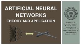
Let ( ) and ( ) be discrete probability functions, such that P (x) and Q(x) are non-zero for 1 . In particular, let Q(x) = 1=N and for some 0 M N let 1 if x = M P (x) = 0 otherwise as shown in Fig. 2.1 for N = 6 and M = 4 (an unbiased die roll, for example). The I-Divergence between P and Q is then (2.20) DI (P; Q) = log(N ) or DI (P; Q) = log(6) 1:79 if taking natural logarithms (about 2.58 bits). P x Qx x 2 f ; : : : ; Ng

8

CHAPTER 2.


1.2

1

P(X)

0.8

0.6

0.4

0.2

0

1

2

3

4

5

6

X

Fig. 2.1: I-Divergence between Discrete Distributions Example: I-Divergence between Gaussians

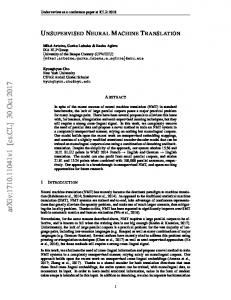
Let p and q be normal distributions with respective means p and q and variances p2 and q2, i.e. 1 exp 1 (x p)2 p(x) = q 2 p2 2p2 and similarly for q. The I-Divergence between p and q is ! q2 1 (p q )2 1 p2 1 DI (p; q ) = (2.21) 2 log p2 + 2 q2 + 2 q2 1 ! p q )2 1 p2 1 ( = H (q) H (p) + 2 2 + 2 2 1 : (2.22) q q In particular, if q = 0, q2 = 36, p = 4 and p2 = 1 (Fig. 2.2), DI 1:53 (2.20 bits). 2.2

Information Theory in Psychology

Ever since Shannon's \Mathematical Theory of Communication" [Shannon, 1948] rst appeared, information theory has been of interest to psychologists and physiologists, to try to provide an explanation for the process of perception. Attneave [1954] proposed that visual perception is the construction of an economical description of a scene from a very redundant initial representation. He suggested that most of the information in a scene is concentrated around lines and corners, i.e. the regions where the content of the scene changes. Thus it is possible that perception process is performing some sort of data reduction on received sensory input, to enable it to be processed and stored more easily. The maximum rate at which a person can transmit information has been measured to be around 30 or 40 bits per second [Attneave, 1959], while Kelly [1962] measured the informationcapacity of a single retinal channel to be 109 bits per second. He suggested that the visual system \takes advantage of the input statistics to perform various coding operations", to reduce some of this high data rate to something more manageable. Barlow [1961, 1987] has suggested that lateral inhibition (in the retina, for example)

2.3.

9

UNSUPERVISED NEURAL NETWORKS

0.4 0.35 0.3

p(x)

0.25 0.2 0.15 0.1 0.05 0 -20

-15

-10

-5

0

5

10

15

20

x

Fig. 2.2: I-Divergence between Gaussian Distributions can help, by reducing the redundancy of an image, so the same amount of information can be represented more eciently. This use of information theory has had its detractors. Green and Courts [1966] for example, argued that information theory could not be used in the consideration of perception, since there is no objective àlphabet of symbols' and also no objective transition probabilities. Despite these arguments, the feeling that information theory is a useful tool for examining perception has continued [Strizenec, 1975]. Leeuwenberg [1978] and Mellink and Buart [1987] have continued with this idea with their `Structural Information Theory', which has primarily been used in connection with the perception of simple visual patterns. 2.3

Unsupervised Neural Networks

One obvious application of information theory is to measure the information capacity of associative memory networks, such as the Hop eld network [Abu-Mostafa and Jaques, 1985]. Of more interest to us, however, is the use of an information measure to suggest learning algorithms for unsupervised neural networks [Becker, 1991]. 2.3.1 Cross-Entropy Maximisation: \G-Max"

An early technique in this area, G-Maximization, was suggested by Pearlmutter and Hinton [1986]. Their model has N binary inputs xi with corresponding weights wi, i = 1; : : : ; N and a single binary output y. The state of this output unit is determined stochastically in a similar way to those in the Boltzmann machine [Ackley et al., 1985]. The probability that the output state is \1" is ! N X (2:23) Py (1) = wi xi i=1

where the () is the logistic sigmoid function 1 (x) = 1 + exp( x) : They suggested that to discover regularities in the input patterns,

(2:24)

10

CHAPTER 2.


\: : : the unit should respond to patterns in its inputs that occur more often than would be expected if the activities of the individual input lines were assumed to be independent." To this end, they chose as their target function the cross-entropy distortion 1 X P (y ) G= P (y )log Q(y ) y=0 between the true output probability distribution P (y), and the ìndependent' probability distribution Q(y) of the output, if the inputs are assumed to be independent. This can be dierentiated with respect to each of the weights wi, and a hill-climbing technique used to nd the maximum. The algorithm is run in two phases: rst with real data to accumulate statistics about P (y); and then with simulated data with inputs generated independently to accumulate statistics about Q(y ). For this second phase, the inputs have the same likelihood of being on or o individually as they did in the rst phase, but now independent of the state of the other input lines. When this was tested on a 10 10 \retina" exposed to randomly positioned and oriented edges, the output unit typically developed an centre-surround antagonistic response: the unit developed a positive (or negative) reponse to receptors in the center of the retina, with the opposite reponse to the surrounding annulus. This model was dicult to extend to more than one unit, since some other scheme has to be used to prevent them all learning the same features of the input. Another possible disadvantage was the requirement to generate synthetic input data during the second pass. It seemed that a dierent approach would be required for networks with many output units. 2.3.2 Maximising of Mutual Information between Output Units: \IMax"

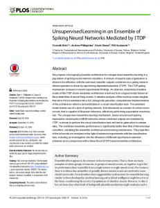
More recently, Becker and Hinton [1989] suggested that the information between output units could be used as the objective function for an unsupervised learning technique (Fig. 2.3). In a visual system, this scheme would attempt to extract higher-order features of the visual scene which are coherent over space (or time). For example, if two networks each produce a single output from two separate but neighbouring patches of a retina, the objective of their algorithm is to maximise the mutual information I (Y1; Y2) between these two outputs. A steepest-ascent procedure can be used to nd the maximum of this mutual information function, both for binary- and real-valued units. One application of this principle is the extraction of depth from random-dot stereograms [Julesz, 1971]. Nearby patches in an image usually view objects of a similar depth, so if the mutual information between neighbouring patches is to be maximised, the outputs from both output units y1 and y2 should correspond to the information which is common between the patches, rather than that which is dierent. In other words the outputs should both learn to extract the common depth information rather than any other property of the random dot patterns. For binary-valued units, with each unit similar to that used by the G-max scheme described above, the mutual information I (Y1; Y2) between the two output units is I (Y1 ; Y2 ) = H (Y1 ) + H (Y2 ) H (Y1 ; Y2 ) (2:25) so if the probability distributions P (y1), P (y2) and P (y1; y2) are measured, this mutual information can be calculated directly. Of course, it is sucient to measure P (y1; y2) only, since ( )=

P y1

1 X y2 =0

(

P y 1 ; y2

)

and similarly for P (y2). The derivative of (2.25) can be taken with respect to the weights in the network for each dierent input pattern, so enabling the steepest-ascent procedure to be used.

2.3.

11

UNSUPERVISED NEURAL NETWORKS

y1

y2 Maximise mutual information

Retina

Fig. 2.3: Maximising Mutual Information between Output Units

12

CHAPTER 2.


For real-valued outputs it would be impossible to measure the entire probability distribution ( ; ), so instead it is assumed that the two outputs have a Gaussian probability distribution, and that one of the outputs is a noisy version of the other, with independent additive Gaussian noise. In this case, the information I (Y1; Y2) between the two outputs can be calculated from the variances of one of the outputs (the `signal') and the variance of the dierence between the outputs (the `noise') as 2 1 I (Y1 ; Y2 ) = log 2 Y1 (2:26) 2 P Y1 Y2

where Y2

Y1 Y2

is the variance of the output of the rst unit, and Y21 Y2 is the variance of the dierence between the two outputs. There are also alternative symmetrical objective functions which can be used instead [Becker and Hinton, 1989, Becker, 1991]. Now, if we accumulate the mean and variance of both Y1 and Y1 Y2, it is possible to nd the derivative of (2.26) for each input pattern, with respect to each weight value. Thus the weights in the network can be updated in a steepest-ascent procedure to maximise I (Y1; Y2), or at least the approximation to I (Y1; Y2) given by (2.26). Becker and Hinton found that unsupervised networks using this principle could learn to extract depth information from random-dot stereograms with either binary- or continuous-valued shifts, as appropriate for the type of outputs used, although in some cases it helped to force the units to share weight values, i.e. enforcing the idea that the units should calculate the same function of the input. They generalised their scheme to allow networks with hidden layers, and also to allow multiple output units, with each unit maximising the mutual information between itself and a value predicted from its neighbouring units. This latter scheme allowed the system to discover an interpolation for curved surfaces. More recently, Zemel and Hinton [1991] have generalised this procedure to allow for more than one output per module. In their network, they use 4 outputs per unit to attempt identify four degrees of freedom in 2-dimensional objects: horizontal and vertical position, orientation, and size. The objects used were simple dipole objects with a left half and a symmetric right half. The mutual information measure is now 1 det(Y1+Y2 ) I (Y1 ; Y2 ) = log (2:27) 2 det(Y Y ) 1

1

2

where Y1+Y2 is the covariance matrix of the sum of Y1 and Y2 (now vectors, of course), and Y1 Y2 is the covariance matrix of their dierence. By measuring the degree of mismatch between the two representations, the model can tell roughly how much one half of an object is perturbed away from the position and orientation which is consistent with the other half of the object.

2.3.3 Minimising Information Loss

Both of these procedures outlined above use information theory measures in their formulation, but neither is concerned directly with the actual information transmitted through to the output units about the input. Rather they attempt to discover regularities in the input data to a single output unit (G-Max) or between dierent output units (I-Max). An alternative to these procedures is to try to minimise the information loss across a network [Plumbley, 1987, Plumbley and Fallside, 1988a] I = I (X ; ) I (Y ; ) (2:28) where I (X ; ) is the information in the input of the network about some feature variable , and I (Y ; ) is the remaining information at the output of the network about this feature variable. For most purposes, this is equivalent to Linsker's \Infomax" principle [Linsker, 1988b, Linsker, 1988a] that the information transmitted through the network I (Y ; ) should be maximised; however, we prefer the information loss formulation, (for reasons which should become apparent when we consider non-Gaussian distributions). Linsker has successfully applied his Infomax principle to linear lters [Linsker, 1989a] and the generation of Kohonen-like ordered maps [Linsker, 1989c].

2.4.

13

INFORMATION LOSS ACROSS A NETWORK

It is also possible to maximise I (Y ; ) more directly, in a supervised learning scheme, where we have access to the feature variable as a teacher. We maximise I (Y ; ), hence minimising I , by making Y follow as closely as possible. In the following, we shall investigate the consequences of attempting to minimise information loss I , initially for supervised neural networks, and then in unsupervised networks. We shall see that some familiar learning algorithms can be shown to decrease information loss as they proceed, and it is possible to modify old algorithms, and design new ones, in order to ful l this requirement to minimise the information loss across the network. 2.4

Information Loss across a Network

2.4.1 Properties of Information Loss

The simple information loss measure which we are considering has several useful properties which help with our consideration of unsupervised (and supervised) networks. Let us write I (X; Y ) = I (X ; ) I (Y ; ) (2:29) for the information lost about across the transform X ! Y .

Non-negative across a transform

Firstly, for any transform Y = f (X ), from (2.13) we know that I (Y ; ) I (X ; ), so the expression (2.29) is non-negative, with equality when f () is reversible.

Non-negative with additive noise

Consider a system with additive noise Y = X + , where is independent of and X , we can write I (X; Y ) = I (X ; ) I (Y ; ) = H (X ) H (X; ) (H (Y ) H (Y; )) : (2.30) Since is independent of X and , H (X; ) = H (X )+ H (), and H (X; ; ) = H (X; )+ H (). Thus, remembering that the transform (X; ) ! (X; Y ) has determinant 1, we can rewrite (2.30) as I (X; Y ) = H (X; ) H (X; ; ) H (Y ) + H (Y; ) = H (X; Y ) H (X; Y; ) H (Y ) + H (Y; ) = I (X ;(Y; )) I (X ; Y ) 0 (2.31) again from (2.13), since Y is a transform from the pair (Y; ). This result suggests that unsupervised learning to minimise this information loss, given that only X and Y are available (and not ), may be possible under certain circumstances. If we could keep the term I (X ;(Y; )) xed, or at least place an upper bound on it, by maximising I (X ; Y ) we could minimise or place a lower bound on I (X; Y ). We shall return to this idea later, when we consider principal component analysing networks.

Additive in series

Over a chain of n 1 networks transforming X1 to X2; ; Xn 1 to Xn, we can verify that I (X1; XN ) =

nX1 i=1

I (Xi; Xi+1)

(2:32)

14

CHAPTER 2.


so the information lost across any transform in this series can never be regained. Each transform should therefore attempt to minimise its own information loss, to try to minimise the information lost over the whole chain. Of course, in trying to minimise the information loss across itself, it is possible that an early network in the chain may transform the data into a form which would make it more dicult for a later network to minimise its own information loss. For example, suppose the rst network in a chain has two outputs, and learns that it can minimise its information loss if it sends all its data down only one of its outputs. Also suppose that the following network always ignores the output chosen by the preceding network: its algorithm doesn't allow it to `listen' to that particular input. In this case, the whole system would do better if the rst network chose a suboptimal solution, allowing the second network to extract at least some information from the input which it does listen to. However, provided we make certain symmetry assumptions about the classes of functions that the networks are allowed to take (e.g. the networks should be capable of using all available inputs), this problem should not arise. 2.4.2 Minimisation of Information Loss by Supervised Learning

A direct method to minimise the information loss I (X; Y ) = I (X ; ) I (Y ; ) is to attempt to maximise I (Y ; ) if the is available at the output of the network as a teacher. The information in the input to the network, I (X ; ) is independent of the network weights, but the output Y is determined according to the network function fW () for a weight vector (or matrix) W , such that Y = fW (X ) so the information I (Y ; ) at the output of the network is dependent on fW , and hence W . Now, we can write I (Y ; ) = H ( ) H ( jY ) where H ( ) is xed, if we minimisethe uncertainty in given Y , H ( jY ), we will in turn minimise the information loss I (X; Y ). For supervised learning, we try to minimise this term H ( jY ) by making Y follow as `closely' as possible. Bayesian classi cation: Two classes

Suppose that the output from our transform is a single binary random variable Y , which is attempting to match a binary target (i.e. both Y and take values in f0,1g). De ne the Bayesian error Y =

= 01 ifotherwise from which we can verify that H ( ; Y ) = H (; Y ) so H ( jY ) = H ( ; Y ) H (Y ) = H (; Y ) H (Y ) = H (jY ) (2.33) H () with equality when is independent of the estimator Y . Now, if pi = Pr( = i) for i 2 f0; 1g, we can write 1 X H () = pi log pi i=0

2.4.


15

which monotonically increases with the Bayesian probability of error, p1, if p1 1=2. Thus if we minimise the probability of error, we will minimise the upper bound on the information loss about

across any network with output Y . By minimising the probability of error, we adopt a minimax strategy to the minimisation of information loss across the transform. Bayesian classi cation:

n

classes

The analysis for n classes is more involved. The distribution of `wrong' classes becomes important, with the most eective minimisation when the errors are as evenly distributed between the classes as possible, or at least, the errors are consistently distributed amongst the other classes. To see this, consider a set of n possible outcomes 1; : : : ; n, with an error function = (

Y )mod n. Now, H () = p0 log(1=p0 ) + (1 p0 )log(1=(1 p0 )) + (1 p0 )H (j 6= 0) where H (j 6= 0) is the conditional entropy of given that we know that 6= 0, i.e. we know that some error was made. In other words, this is the entropy of errors within the `wrong' classes. When H (j 6= 0) is maximal, i.e. when the probability of making an error into any of the other classes is equal, minimising the Bayesian error probability will bound the information loss, provided the probability of error Pr( 6= 0) (n 1)=n. However, if the distribution of errors is not uniform, the information loss will not be tightly bound in this way. In the extreme case of many classes, where there is an implicit ordering among the classes, Bayesian classi cation would no longer appropriate. This has implications for speech processing, for example, where it is common to attempt to minimise the probability of a phoneme error, where the number of possible phonemes could be as high as 60 or more [Robinson and Fallside, 1990, Lippmann, 1989]. For this task, it is highly likely that the error distribution is not uniform, and not consistent for each true phoneme, since it is easier to confuse `close' vowels than some consonants, for example. If the minimum Bayesian error probability is the nal output required from the system, this is no problem, but in this case we might like to use this phoneme recogniser as a building block as part of a word or sentence recogniser. Minimising the Bayesian error probability at the phoneme level will not guarantee that we minimise the information loss across the phoneme recogniser stage, and we may not get the performance we would like from a complete system as a word recogniser. Essentially, the `pick the biggest' transformation loses a lot of information, and if we would like the whole system to perform better, we should keep more for the next stage. One way of doing this is to keep the probabilities of some N > 1 most probable outputs: this will be optimal if the probabilities of making an error to any of the other n N outputs are equal, and will thus be a better t than if we simply kept the identity of the top one. This idea is related to the `N-BEST' technique used in speech recognition [Young, 1984, Schwartz and Austin, 1991].

2.4.3 Minimising Information Loss by Minimising Distortion

In addition to the Bayesian error minimisation techniques outlined above, we can also bound our information loss target by minimisation some distortion measure between the output and target values, in the case of continuous-valued outputs. This type of distortion minimisation is used when training Multi-Layer Perceptrons with the Error Back-Propagation algorithm, for instance [Rumelhart et al., 1986].

General Mean Squared Error

If we write the error =

we have

, where Y is the output of the network, and is the target, then H ( jY ) H () with equality if is independent of Y . If we could minimise H () directly, we could then bound the information loss as before, by bounding H ( jY ). Unfortunately, in contrast to the discrete Y

16

CHAPTER 2.


case, it is no longer possible to minimise H () directly. However, we can bound the value of H () by minimising the mean squared error, as follows. If the covariance matrix of is given by = E (T ), then the entropy of is bounded by 1 H () log (2e)N det 2 where N is the dimensionality of the output vector (and hence ), with equality if has a multivariate normal distribution [Shannon, 1948]. Also, since we can bound the value of det by bounding the trace, tr, we can bound H () by bounding the mean squared error DMSE ( ; Y ) = E (jj2 ) = tr() providing has zero mean. The best t we will get on all of these bounds occurs when the error is zero mean spherical Gaussian, and independent of the estimator Y . If these conditions are not satis ed, the bounds so produced will not be tight, and we may not minimise the information loss even if we do minimise the mean squared error. We can summarise the bounds we use in the I-divergence diagram, or I-Diagram in Fig. 2.4. The vertices give probability distributions, and the edges give I-divergences between the probability distributions at the two edges (with the `true' distribution at the arrow head). In this diagram, the notation Y P (Xi ) i

represents the probability distribution over the vector X = (X1; : : : ; XN ), with P (X ) = P (X1 )P (X2 ) P (XN ): Since the probability distributions indicated are all maximumentropy (or minimumcross-entropy) distributions, the I-divergences on the arrows on this diagramare additive, even though I-divergences are not additive in general [Csiszar, 1975, Shore and Johnson, 1981]. We can see from this diagram that there is a large amount of room for `slop': i.e. minimising the mean squared error will not guarantee to maximise I ( ; Y ), at the bottom of the diagram, unless the error = Y is independent spherical Gaussian. Matching probabilities

If the target values for in the previous section represent a probability vector, the situation is simpler than in the general case above. In particular, it is often the case that one of the target values is 1 (on), representing the class to be associated with the network input, while the other outputs are o (zero). In fact, the mean squared error will be minimised when the outputs form the a-posteriori Bayesian probability estimates of the output class given the input, Yi = P ( ijX ), if this is possible [Hampshire and Pearlmutter, 1990]. The same is true for the component-wise cross-entropy measure introduced by Solla, Levin and Fleisher (CE-SLF) [Solla et al., 1988]: N X DCE SLF ( ; Y ) =

i log Yii + (1 i)log 11 Yii : i=1 If the network is not suciently ` exible' to form the exact a-posteriori probabilities, it will attempt to form a minimum mean-squared-error or minimum cross-entropy approximation to this value, depending on the distortion measure in use. Fig. 2.5 shows an I-diagram for the CE-SLF distortion measure, from which we can see that this is simpler than the general case for minimum mean squared error. In this case, this measure attempts to minimisethe sum of the informationloss across the transform from X to each output Yi. This does not guarantee that a `pick the best' from the output of a network trained using CE-SLF will have a Bayesian error rate less than one trained with the normal MSE measure. In fact, the opposite may be true, since Bayesian probability of

2.4.

17


(DMSE ( ;Y ))

(0 )

1

!

N ; N

(0 )

N ; N

P

? ? y

1=N Pi( i

Yi

? ? y

Q

iP

P

( i

P

Yi

? ? y

(

Y

( )

? H ( )? y

0

)21=2

)

)

N

P i

I ( i Yi ;Yi )

I ( Y ;Y )

!

I

Q

!

( ; Y )

!

P

iP

( ijYi) ? ? y

( jY ) = P (

P

( jY )

Y jY

) H ( jY )

! P ( jY; )

0

Fig. 2.4: I-diagram for General Mean Squared Error. In this form of I-diagram, the vertices are each labelled with a probability density (PD). The arrows between edges, where labelled, give a particular interpretation for the I-divergence between the PDs at each end of the arrows: for example, the I-divergence between P ( Y ) and P ( Y jY ) is I ( Y ; Y ), the mutual information between Y and Y . If the label on an arrow appears in parenthesis (as does DMSE( ; Y ) on this diagram), this is not the true I-divergence itself, but a number which determines the I-divergence. A special vertex marked \0" denotes a discrete probability distribution which is fully determined (i.e. P (xi) = 1 for some i). Similarly, \ 1" is used to denote a probability density which is a delta function. This diagram shows that minimising the mean squared error distortion, at the top of the diagram, only loosely maximises the mutual information I ( ; Y ), at the bottom of the diagram. In particular, the form of the PD P ( Y ) will determine how loose the connection between DMSE( ; Y ) and I ( ; Y ) will be: i.e. how much `slop' exists in the system.

18

CHAPTER 2.

Q

i ((1

? ? y

) )

Yi ; Yi

DCE

P Q

iP

P

( ijYi)

i

SLF


( ;Y )

C

!

Q

i ((1

I (X; Yi)

!

I ( ;X )

( )

P

P

H ( i jX ) Q

!

Q

iP

Q

( ijX )

P

H ( i jX )

!

? D ( ; i jX )? y i I

!

? H ( )? y

( ijX )); P ( ijX ))

Q

((1 i); i)

Q

H ( jX )

( jX )

i

!

0

P

P

( ijX; i)

( jX; )

0 Fig. 2.5: I-Diagram for Solla, Levin and Fleisher Cross-Entropy.

error is the mean-squared-error between two binary vectors, each with one component at one and the others at zero. From our information-loss viewpoint, however, the CE-SLF measure represents an improvement over MSE. A further improvement can be gained if we realise that the CE-SLF measure is treating outputs as individual probability estimators, with the òn' probability being Yi, and the ò' probability being 1 Yi. In this case, we need only ensure that 0 Yi 1 for thisPto be a valid probability distribution. If, however, we were to normalise the outputs so that i Yi = 1, then we could compare the probability vector Y to the actual probability vector directly, using the distortion measure N X DCE MMI ( ; Y ) =

i log Yii (2:34) i=1

as shown in Fig. 2.6. Bridle [1990] has taken this approach, using his `softmax' function (Y 1 ; : : : ; Y N )

DCE

MMI

( ;Y )

? ? y

P

( )

? H ( )? y

I

( ; Y )

!

P

( jY )

0

! ( 1 ; : : : ; N )

H ( jY )

!

P

( jY; )

0 Fig. 2.6: I-diagram for CE-MMI distortion measure

Oi ) = Pexp( (2:35) Oj ) exp( j where Oi are the activations of the nal layer units. This ensures the outputs are positive and sum to one, and `probability scoring' which is the cross-entropy measure in (2.34), and is related to MMI (Maximum Mutual Information) training in Hidden Markov Models (HMMs) [Bahl et al., 1986]. Yi

2.4.


19

This softmax function combines well with the cross-entropy measure, since if Y is given by (2.35), and the error S = E (DCE MMI ( ; Y )) ; then [Bridle, 1990] @S = i Yi (2:36) @Oi which is a generalisation of a similar result for the combination of the logistic sigmoid function with the CE-SLF distortion measure. The Perceptron Learning Procedure from Cross-Entropy

This result of (2.36) above is independent of any scaling applied to Oi before the softmax function, i.e. if we use exp(kOi) Yi = P (2:37) j exp(kOj ) for any constant k. For some small , provided jOi Oj j for all i and j , and for all input presentations to the network, as k ! 1 we get 1 if Oi > Oj for all j 6= i Yi ! 0 otherwise but the error derivative remains proportional to the original, i.e. 1 @S = i Yi k

@Oi

so if the outputs i are either zero or one, the derivative (scaled by 1=k) will be 0 if the network output is correct, and 1 if it is incorrect. For the Gaussian radial basis functions (RBFs) considered by Bridle [1990], this leads to a rule which moves the centres of the RBFs until they are at the centroids of the incorrectly classi ed data. It is easy to see, however that the same reasoning will lead to the Perceptron Learning Rule, i.e. for the single-output system O = WTX with 1 if O > 0 ; Y = 0 otherwise the learning rule if Y =

W = 0( Y )X otherwise is equivalent to a steepest decent procedure using the componentwise cross entropy measure DCE SLF ( ; Y ) and the sigmoid output function 1 Y = 1 + exp( kW T X ) as k ! 1. 2.4.4 Information Loss and Infomax

The minimisation of information loss criterion [Plumbley, 1987, Plumbley and Fallside, 1988a] for a network from X to Y , I (X; Y ) = I ( ; X ) I ( ; Y ) and Linsker's Ìnfomax' criterion [Linsker, 1988b, Linsker, 1988a], i.e. maximisation of I ( ; Y )

20

CHAPTER 2.


are apparently identical, since I ( ; X ) is independent of any transform we choose from X to Y . The advantage of minimising loss of information rather than simply maximising nal information arises when we only measure certain parameters of the probability distributions of X and Y : commonly we only measure the covariance matrices of these distributions. Consider the single system in Fig. 2.7. For this system, we have X = +X , and Y = X +Y ,

-

6

X -

6

Y -

X Y Fig. 2.7: Information loss with additive noise i.e.

= + (X + Y ) where X and Y are independent additive noise terms. Y

Infomax for non-Gaussian signals

For the Infomax criterion, we will be measuring I ( ; Y ) = H (Y ) H (X + Y ) with a view to maximising this quantity. Since X and Y are xed, this will be equivalent to maximising H (Y ). Suppose that for simplicity we assume Y to be zero mean, and we only measure the variance of Y , Y2 = E (Y 2). This will place an upper bound of 1 Hmax (Y ) = log 2eY2 2 on the entropy H (Y ), thus placing an upper bound on the transmitted information I ( ; Y ). This upper bound will be achieved for the Gaussian density N (0; Y2 ), but any other distribution will have less entropy, and hence less transmitted information. Hence if we only measure the variance, we can only maximise the transmitted information if the output Y is Gaussian: for any other probability distribution for Y , all we know is that we have maximised the upper bound on I ( ; Y ). Information loss for non-Gaussian signals

If instead we consider the information loss I (X; Y ) = I ( ; X ) I ( ; Y ) (2.38) = H (X ) H (Y ) H (X ) + H (X + Y ) (2.39) we can improve upon the situation outlined above. Essentially, if the noise term Y is Gaussian, for Y to be non-Gaussian, X must be non-Gaussian also. So if I ( ; Y ) is less than the maximum value for a particular variance measurement, so I ( ; X ) will also be less than its maximum. Let us look at the way that I (X; Y ) varies with pX (X ) such that the constraints Z

( ) =1

pX x dx

and

E X2

( ) = X2

(2:40) (2:41)

2.4.

21


hold. We can use the calculus of variations to nd the maximum information loss for a given Y , and hence X . Provided the output noise Y is Gaussian with zero mean, we nd Z

d dpX x

(2.42) ( ) I (X; Y ) = log pX (x) + p log pY (x + ) + 1 = log pX (x) H (Y ) DI (p ; pY x) + 1 (2.43) where pY x() = pY ( + x), and DI (; ) is the I-divergence measure described in section 2.1.5. Note that the form of the input noise X does not appear in this expression: it need only be additive. To maximise I (X; Y ) under the constraints (2.40) and (2.41), we should maximise Y

Y

J

= I (X; Y )

Z

Z

()

pX x dx

x2 pX x dx

()

over pX (x), for lagrange multipliers and . This leads to the condition = log pX (x) H (Y ) DI (p ; pY x) + 1 x2 = 0 which we can verify is satis ed for Gaussian output noise ! 2y 1 1 exp 2 2 p ( Y ) = q 22 when 1 1 x2 pX (x) = p 2X2 exp 2 x2 : If the second derivative of J is negative de nite in the direction of our constraints, i.e. d J dpX x

()

Y

Y

Y

y

=

Z Z

(2:44)

2

(pX (x))(pX (x0)) dpX (x)ddpX (x0) J dx dx0

(2.45) (2.46) 0 for any pX (X ) = pX+ (X ) pX (X ) such that (2.40) and (2.41) hold for both pX+ and pX , then the solution of (2.44) will be a maximum for the information loss. For this second derivative, we nd Z 1 1 p ( + x x0)d d2 0 J = (x x ) + p () dpX (x)dpX (x0 ) pX (x) pY ( + x) Z (x x0 ) p (y x)p (y x0 ) = + (2.47) dy pX (x) pY (y ) F

Y

Y

Y

which is symmetrical in x and x0. Thus we get Z Z Z (pX (x))(pX (x0)) (x F = = where and

Z

(pY

(y))2

()

pY y

Z

dy

(x))2

(pX pX (x) ( )=

Z

pY y

pY (y) =

Z

x0 pX x

()

Y

) + p (y Y

() (

( )pX (y

pY

(

()

x0

) dx dx0 dy (2.48)

dx

pY pX y

)

x pY y pY y

)

d

)

d:

22

CHAPTER 2.


So for the Gaussian to be a maximum, F must be strictly negative, so we must have Z (pX (x))2 dx > Z (pY (y))2 dy: (2:49) pX (x) pY (y ) We can verify that this is possible in the case where pX (x) and pY (y) are approximately constant whenever pX (x) and pY (y) are signi cant, and the noise is small. For Gaussian pX (x), we nd that Z (pX (x))2 dx / 1X and, since the variance of pY (y) would be greater than pX (x), we will have Z

Z

(pX (x))2 dx > (pY (y))2 dy:

This is not a proof that F < 0, but it does lead us to conjecture that F in (2.48) is negative. If this is the case, the Gaussian probability density for X (and hence Y , since Y is Gaussian), would be not only the maximum transmitted information condition, but also the maximum information loss condition. Thus by minimising the information loss for a Gaussian distribution, we would minimise the upper bound on the information loss across corrupting Gaussian noise: a `damage limitation' approach. 2.4.5 Applying Information Loss

In practice, the application of information loss minimisation is essentially identical to Linsker's Ìnfomax' [Linsker, 1989c, Linsker, 1989b], except we bear in mind that if we always deal with Gaussian distributions, we are upper-bounding the loss of information rather than upper-bounding the transmitted information. This upper-bounding also applies when certain components of the input are ignored completely, as we shall see when we consider principal component analysis networks. Most of the following sections on information loss minimisation will concentrate on linear unsupervised learning systems, for analytical tractability. In all these sections, the assumptions that we make about the input noise are always important. Conceptually, these assumptions make up for the fact that we are not allowed access to , which would supply our targets in a supervised learning system.

Chapter 3 Principal Component Analysis Principal Component Analysis is a popular statistical tool for removing redundancy from data in a linear fashion, and deserves special mention. It has various names in dierent signal and data processing elds, including Factor Analysis, (discrete) Karhunen-Loeve Transform (KLT), and the Hotelling Transform in image processing [Watanabe, 1985, Gerbrands, 1981, Gonzalez and Wintz, 1987]. Various unsupervised algorithms have already been suggested for a linear neural network to nd the Principal Components or Principal Subspace of their input data [Oja, 1982, Oja, 1983, Oja and Karhunen, 1985, Williams, 1985, Bourlard and Kamp, 1987, Foldiak, 1989, Sanger, 1989a], so this represents an important aspect of our consideration of unsupervised learning in general. 3.1

Transforming for Principal Components

Consider the N -input, M -output linear network yj

=

N X i=1

wij xi

(3:1)

where xi is the ith input unit, yj is the j th output unit, and wij is the weight connecting the ith input to the j th output. Alternatively, this can be written in matrix notation as (3:2) y = WTx where x is the N -dimensional input vector and y is the M -dimensional output vector, and W is an N M weight matrix (Fig. 3.1). The inputs x are instances of some random variable X with mean x = E (x) and covariance matrix x = E ((x x)(x x)T ). We shall assume for simplicity that x = 0 (we can always force this to be the case by centralizing the input vector to produce a modi ed input x~ = x x before applying the weight matrix). Let i and i, i = 1; 2; : : : ; N , be the eigenvectors and corresponding eigenvalues of the covariance matrix x, where 1 2 N . If M = N , and the columns of W (rows of W T ) are the eigenvectors i in order, then this network is said to perform a Karhunen-Loeve Transform (KLT) on the input vectors x [Gerbrands, 1981]. 3.1.1 Properties of the KLT

Since the covariance matrix x of the zero-mean Tinput vectors is real and symmetric, its eigenvectors i form an orthonormal set. Thus W W = W T W = IN , and the output covariance matrix y = W T xW (3.3) = WTW (3.4) = (3.5) 23

24

CHAPTER 3.

y1 6

y2 6 n

w11

x1

6 n

x2

yM 6

n

6 AK A @I @ 6 AK A @I A @ A @ A A

PRINCIPAL COMPONENT ANALYSIS

n

6 n

@ 6 AK A @I @ 6 AK A @I @ 6 AK A A @ A @ A @ A w A @ A @ A @ A @ A @ A @ A @ A @ A @ A @ A @ A

NM

xN

Fig. 3.1: A Single Layer Linear Network. where

2 6

= 664

1

2

0

0 ...

3 7 7 7 5

(3:6)

N

Thus the output has the properties of Decorrelation The activations of the output units are uncorrelated; and Decreasing Variance The variances of the output units are simply the eigenvalues i of the input covariance matrix, and monotonically decrease with output unit number. The decorrelation property of the outputs is important in Factor Analysis [Watanabe, 1985], since the object here is to attempt to identify independentT factors which combine in a linear fashion to give rise to the observed data. In addition, since W W = IN , the input x can be reconstructed from the output y using (3:7) x = Wy If there are fewer output units available than input units (M < N ) we can simply drop the higher numbered outputs M < j N to give us (3:8) y = WMT x where WM is the N M matrix whose M columns are the rst M eigenvectors of x . The outputs will still be uncorrelated, with WMT WM = IM , but now WMT is not invertible, so we can now only estimate the input from the output x^ = WM y (3:9) with squared error ^)(x x^)T (3.10) SMSE = tr E (x x T = tr x(IN WM WM ) (3.11) =

N X

i=M +1

i :

(3.12)

Since the eigenvalues were chosen to be monotonically decreasing, this represents a least-squarederror (LSE) reconstruction for x from y: the LSE reconstruction property.

3.1.

TRANSFORMING FOR PRINCIPAL COMPONENTS

25

3.1.2 The Projection Induced by WM

If we are only interested in the LSE reconstruction property, and not the decorellation property, we only need to nd the principal subspace rather than all the principal components. To see this, we consider the projection induced by the WM , which describes the principal subspace. If we let PM = WM WMT , we can verify that PM2 = PMTT = PM . Thus PM is an orthogonal projection [Golub and van Loan, 1983] onto the range of WM (In the particular case of N = M , PM = IN ). Now we can rewrite the reconstructed signal x^ as x^ = WM WMT x (3.13) = PM x (3.14) with reconstruction mean squared error as S = tr((I PM )x ) (3:15) Thus PM is the projection on to the principal eigenspace of x. In fact, it can be shown that for any full rank N M matrix W whose columns span the same subspace as any M eigenvectors of x, the LSE reconstruction is given by x^ = P x (3.16) W + = (W T W ) 1 W T , the Moore-Penrose psuedo-inverse of W where P = (W +)T W T , with T [Strang, 1976] (where (W W ) 1 exists). This gives the same reconstruction squared error as above. Thus if we are only interested in the minimum squared error, we can use any weight vector which induces the same projection PM onto the M -dimensional principal eigenspace, i.e. any matrix W whose columns span the same subspace as the M principal eigenvectors of x. Of course, using any general matrix W which spans the principal eigenspace is not guaranteed to give us uncorrelated outputs. If the object of the exercise is simply to produce an output y which can be used to reconstruct the input with least squared error, any correlation at the outputs is of no consequence. We shall re-examine this point later. 3.1.3 Problems With PCA

The application of Principal Components Analysis to real data suers from the scaling problem, i.e. the principal components produced depend on the way the data is scaled. As a simple illustration, consider the data shown in Fig. 3.2. The data points have 2 parameters, and we wish to reduce this to a single parameter using PCA. Now, if we scale the axes as shown in Fig. 3.2(a), the apparent single principal component is the one in the direction of the axis x2. However, if they are scaled as shown in Fig. 3.2(b) the apparent principal component is the one in the direction of the axis x1 . This type of problem is also evident in other forms of data classi cation tasks, such as cluster analysis [Hand, 1981, p157]. Of course it would not normally be useful to attempt PCA on this data, since the values on the two axes are independent in this case, but it does serve to illustrate an extreme case of the problem. When the axes are similar types of data, measured over the same values, the obvious solution to this is simply to use 1 : 1 relative scaling between the axes. But what if the measurements are from completely dierent quantities, such as height vs. IQ? To avoid this problem, it is customary to normalise the axes so that each has unit variance [Watanabe, 1985, p212] before attempting Principal Components Analysis. However, the justi cation for this is unclear. Even if the data is normalised so that each component has unit variance, another related problem arises if we have multiple observations of a single data variable. In our hypothetical example, suppose we have only one opportunity to measure height, but four to measure IQ. We have two obvious approaches: 1. Treat the four measurements of IQ as separate, and perform a principal component analysis on the resulting 5-dimensional data. Or;

26

CHAPTER 3.


|

|

| |

|

|

|

|

|

|

|

|

|

|

|

|

|

|

|

|

|

|

|

|

|

|

|

|

|

|

| | |

|

|

|

|

|

| |

|

|

|

|

|

|

|

|

|

|

|

|

|

|

|

|

|

|

|

|

| | |

|

(a)

Fig. 3.2: The Scaling Problem in PCA

(b)

2. Take the mean of the four IQ measurements, and nd the principal component of the remaining 2-dimensional data (using the mean as one of the components). If we do not normalise so that each component has unit variance, we are left with our original scaling problem of how to scale the data appropriately. However, if we do normalise the variance of the data, the two approaches outlined above are not equivalent, and will give an inconsistent value for the principal component. To try to resolve these problems, we shall now consider principal component analysis from an information theory viewpoint. 3.2

Information Lost by Principal Components Analysis

As for supervised learning networks, we can construct an Information Loss framework [Plumbley, 1987, Plumbley and Fallside, 1988b] for the unsupervised linear system (3.2) y = WTx (3:17) with M < N . Now, we wish to minimise the information loss about the pattern instances ! which are instances of some random variable . These patterns are transformed by the `world', together with some corrupting noise, into the observed input vector instances x to our network. I.e. X = U ( ; U ) (3:18) Unlike the supervised case, we can make no observations of the patterns , so cannot minimise the information loss directly. We can make no further progress unless we can make some assumption about the relationship between and X . The assumption we make is that the input X can be considered to be corrupted by spherical additive normally distributed (Gaussian) noise X , so that an input instance is generated according to (3:19) x = !x + x where !x represents the pattern information in x before corruption by the noise (Fig. 3.3). Thus we have independent equal variance noise on each input. The output vectors y are assumed to contain no additional noise, so (3.20) y = WTx = !y + y (3.21)

3.2.

INFORMATION LOST BY PRINCIPAL COMPONENTS ANALYSIS

27

world !x -

6

x

x

-

WT

y -

Fig. 3.3: Additive Input Noise

where !y = W T !x and y = W T x. The information loss across the network, I (X; Y ) = I (X ; ) I (Y ; ) (3:22) where I (X ; ) and I (Y ; ) are the information in the input to the network and the output from the network respectively, about the patterns . If we could measure the probability distribution of X , PX (x) directly, we could ignore I (X ; ), which is not a function of W . By using a W such that I (Y ; ) is maximised, we minimise our information loss I (X; Y ). As an example, let us restrict ourselves for the moment to unitary matrices W T , i.e. matrices T such that W W = IM . Since the output y is corrupted by additive noise only, we know that (3:23) I (Y ; ) = H (Y ) H (Y ): ButT since W T W is unitary and the input noise x is spherical Gaussian, the output noise y = W x is also spherical Gaussian with covariance independent of W , so H (Y ) is independent of W also[Plumbley and Fallside, 1988a]. It remains for us to nd a unitary W so that H (Y ) is maximised. To maximise the true H (Y ) would require us to accurately measure the true input probability distribution PX (x), and deduce which W would give rise to a maximal H (Y ) given this PX (x). Although this measurement may be possible for certain discrete distributions, for a general distribution this would be impractical, since measuring PX (x) accurately would be out of the question. In addition, once PX (x) had been measured, nding a W to maximise H (Y ) would not be a trivial task in itself. One possibility is to make some assumption about the input probability distribution. For example, we could assume that X is normally distributed with zero mean so that PX (x) = N (0; x ). Linsker [1988a] points out that in this case the information I (Y ; ) is maximised for a one-output system (M = 1) when the weight vector W is in the direction of the principal component of x. In fact, for an M -output network, the information I (Y ; ) is maximised for normally distributed X when W spans the M -dimensional principal subspace of x. So for a zero-mean Gaussian input signal, the information loss across the network will be minimised when the outputs are the M principal components of the input, or some output which covers the same subspace. With this assumption that the input signal is normally distributed with zero mean, it is sucient to measure its covariance matrix x to completely determine the probability distribution PX (X ). Unfortunately, this is apparently a `best-case' assumption, which does not necessarily hold for any other input probability distribution. For any distribution PY (y) with covariance matrix y = W T xW , except for the Gaussian distribution with this covariance, the entropy H (Y ) will always be less than the entropy of the Gaussian distribution with this covariance [Shannon, 1948]. Therefore the information I (Y ; ) in (3.23) will always be less than the information for the equivalent Gaussian signal (call this I (Y ; )). We have found an upper bound on the information which could be transmitted through the network, so we have maximised the information capacity of the system, but there is no guarantee that a non-Gaussian signal will achieve this capacity. In game-theoretic terms, Nature could conspire against us, so that although the direction we

28

CHAPTER 3.


chose was the principal component, it would not be the direction with maximum information. Formulated in this way, the principal component analysis approach does not appear as useful as it might be. 3.2.1 An Upper Bound on Information Loss

Fortunately, we can take another approach to the problem. If the signal at the output is nonGaussian, then the signal at the input must also be non-Gaussian. So, for a given input covariance I (Y ; ), the the input information x, if the output information I (Y ; ) is less than the capacity I (X ; ) will also be less than the input information I (X ; ) for the equivalent Gaussian input signal. By considering the information loss I (X; Y ) in (3.22) rather than the transmitted information I (Y ; ) alone, it is possible to bound the information loss for any input probability distribution, given that only the input covariance matrix x is measured. In other words, we wish to place the lowest bound on the information capacity lost from the input to the output, instead of placing the highest bound on the information capacity at the output itself. Noting that since Y is a function of X , we have I (X ; ) = I (X; Y ; ), our information loss I (X; Y ) = I (X; Y ; ) I (Y ; ) (3:24) Let us express the input X as the sum of two terms X = Xy + Xy (3:25) where Xy = W T (W T W ) 1Y (assuming W full rank) so that Xy = P X with P an orthogonal projection. Observing that H (X; Y ) H (X; Y; ) = H (Xy; Y ) H (Xy; Y; ) (3:26) since the determinants of both transforms are equal, after a little manipulation we get I (X; Y ) = I (Xy; Y; ) I (Xy; Y ) (3.27) I (Xy; Y; ) (3.28) I (Xy; ) (3.29) since I (A; B) I (A; f (B)) for any f (). The rst inequality is an equality if Xy is independent from Y . As before, we can write Xy = X + X (3:30) with the obvious interpretation, leading to I (Xy; ) = H (Xy) H (X ): (3:31) Now X = (I P )X , so provided W remains full rank, the rank of the orthogonal projection (I P ) remains constant, so H (X ) remains constant. It remains for us to minimise H (Xy). For a Gaussian distribution, this is minimised if Xy consists of the smallest N M components of X , i.e. the components remaining after the M principal components have been removed. This, then is the principal component analysis solution, and coincides with the minimum mean squared reconstruction error tr(Xy). Any other probability distribution for Xy will have an entropy not more than this value, so the information loss I (X; Y ) will be upper-bounded by the information loss for the equivalent Gaussian distribution. Thus the solution for W T which spans the same space as the M principal components of X is not only the solution for maximum information capacity I (Y ; ), but also the solution for the lowest bound on the information loss, I (X; Y ). So although we may not be able to guarantee that the transmitted information is maximised, we can be sure that the information lost by the network has been bounded as tightly as possible, given the parameters which we have measured. y

y

y

y

y

3.3.

29

NEURAL NETWORK ALGORITHMS FOR PCA

3.2.2 Implications for the Scaling Problem

We have shown that the technique of Principal Components Analysis, or the use of any transformation matrix spanning the same subspace as the principal components of a distribution, will place an upper bound on the information lost by that transformation, provided there is additive spherical Gaussian error on the input vectors. In fact, it is possible to relax this condition slightly [Plumbley and Fallside, 1988a], provided that the entropy of X , the component of the input noise X which is not a function of the output Y , has a lower bound. Of course, this would mean that the information loss upper bound found by the Principal Component Analysis procedure would not be as tight as if H (X ) was constant. We can now view the scaling problem that arises in principal component analysis as the problem of determining an appropriate scaling for the input components to get as close to spherical Gaussian noise as possible, to t as tight a bound as possible to the information loss. If the inputs are all similar, it is reasonable to assume that the noise on all the components is equal, so 1:1 scaling is appropriate. However, if the input components are not measurements of similar quantities, we should attempt to estimate the noise, or uncertainty, in each of the components with respect to the patterns that we are interested in. To see why this is so, imagine that one of the components of the input was virtually noisefree, while the rest had a signi cant amount of noise. The information conveyed by the low-noise component could be much greater than the information conveyed by the other components, even though its variance may be smaller than that of the others. The technique of normalising each input component to unit variance is therefore, in eect, making the assumption that the variance of the noise on each input component is in proportion to the variance of the signal on that input. This is where the inconsistency arises with multiple measurements, such as the four measurements of I.Q. in our example of section 3.1.3. If the mean of the I.Q. measurements are taken before applying principal components analysis, any independent Gaussian error on the individual measurements will give rise to a Gaussian error on the mean of half the variance. Thus the mean value should be scaled to twice the scaling which would have been used for an individual measurement. This gives a consistent way to deal with both of these cases. The proportion of each component in the nal principal component is the same in both cases, provided, or course, that our assumptions about independence of measurements are correct. It suggests that the customary normalisation is often successful when the noise in each component of the data points is approximately in proportion with their variance; this may even be a reasonable assumption to make when no other information is available. However, it is now clear what assumption is being made when this normalisation is used, and in some cases it may be apparent that an alternative scaling is appropriate. y

y

3.3

Neural Network Algorithms for PCA

Our particular interest is in unsupervised learning, so we would like a stochastic approximation algorithm, preferably using only local operations, to nd the principal components or principal subspace. Several such algorithms already exist, with various proofs of convergence [Krasulina, 1970, Oja, 1982, Oja and Karhunen, 1985, Williams, 1985, Sanger, 1989a] as well as similar algorithms designed to nd the minimum eigenvalue of the input covariance matrix, for Pisarenko's `harmonic retrieval' method [Reddy et al., 1982]. We shall see that these algorithms are members of a general class of stabilised Hebbian learning algorithms. By examining the behaviour of the subspace spanned by the transformation matrix W , or rather the behaviour of the orthogonal projection P onto that subspace, we can separate the common Hebbian part of the algorithms from the stabilisation part, and show that they produce an identical algorithm for adapting the projection P . First, let us review the algorithms in this class.

30

CHAPTER 3.


3.3.1 The Algorithms

As before, we have a linear system with yn = WnT xn at the nth time step. The basis of many unsupervised learning algorithms is the Hebbian algorithm, of the form Wn+1 = Wn + n xn ynT (3:32) where n is a small update factor, after D. O. Hebb's postulation that a cell which excites another cell should have its connections strength increased if the cells tend to re together [Hebb, 1949]. Unfortunately, if this rule is used without modi cation, the weights will tend to increase without limit [von der Malsburg, 1973]. One possibility is to renormalise the weights to each output cell, to keep the sum of the weights constant [von der Malsburg, 1973], another to use a hard bound on the weight values [Linsker, 1986], in eect limiting some p-norm of the weight vector.

Krasulina's principal component nder

Krasulina [1970] suggested a stochastic approximation algorithm for computation of the single principal vector (M = 1) Wn+1

=

Wn

+

=

Wn

+

y2 n xn yn Wn T n W n Wn W T xn xT Wn n xn xnT Wn Wn n T n W n Wn

(3.33) (3.34)

where Wn converges to a vector in the direction of the principal eigenvector of x as n ! 1, with certain conditions on x, n and Wn. However, as pointed out by Oja and Karhunen [1985], the weight vector can grow very large with this algorithm. The Oja single principal component neuron

Starting from the Hebbian approach, Oja [1982] observed that the application of the Hebbian algorithm (3.32) in a single output (M = 1) system, followed by a normalisation stage after each time step to ensure the 2-norm of W remains at unity, i.e. ~ n+1 = Wn + nxnyn W (3.35) ~ ~ Wn+1 = Wn+1 =jWn+1 j2 (3.36) can be expanded as Wn+1 = Wn + n xn yn Wn yn2 + O(n2 ) (3:37) which can be written ^nyn + O(n2 ) Wn+1 = Wn + n x (3:38) where x^n = xn Wny. The weight vector W in this algorithm converges to a unit vector which is the dominant eigenvector of x (or the negative of this vector).

Oja and Karhunen algorithm for M components

Oja's algorithm above has been generalised by Oja and Karhunen [1985] to nd the M largest eigenvalues in order with an algorithm based on the Gram-Schmidt orthogonalization (GSO) of the weight matrix Wn at each stage. A simpli ed version of their algorithm is Wn+1 = Wn + n xn ynT Wn diag(yn ynT ) 2Wn UT+ (yn ynT ) (3:39) where UT+() denotes a `strictly upper triangular' matrix operator which sets all the entries on or below the diagonal to zero, and diag() is the operator which sets all entries o the diagonal to zero.

3.3.

31

NEURAL NETWORK ALGORITHMS FOR PCA

Sanger's `Generalized Hebbian Algorithm'

The algorithm above is similar to Sanger's `Generalized Hebbian Algorithm' [Sanger, 1989a], which is also based on a GSO idea: (3:40) Wn+1 = Wn + n xn ynT Wn UT(ynT yn ) where this time UT() is an upper triangular operator which sets all entries below the diagonal only to zero (i.e. the diagonal is retained). Williams' `Symmetric Error Correction' Algorithm

Finally, Oja and Karhunen [1985] mention the algorithm (3:41) Wn+1 = Wn + n xn ynT Wn yn ynT which can be written as ^nynT (3:42) Wn+1 = Wn + n x where x^n = xn WnynT (c.f. algorithm (3.38)). This is the symmetric version of Williams' `Symmetric Error Correction' algorithm [Williams, 1985], and Oja uses this as a learning equation for his `Subspace Network' [Oja, 1989].

3.3.2 A Common Framework

As may already be apparent, all these algorithms for our system yn = W T xn can be written in the form (3:43) Wn+1 = Wn + n xn xnT Wn + Wn n + O(n2 ) where n is some M M matrix which may be a function of Wn and/or xn. The term Wnn is sometimes called a forgetting or weight decay term [Kohonen, 1984], and embodies the intuitive idea that connections in a neural network should decay if they are not used. We shall show that any algorithm in this class leads to identical conditions for convergence of the orthogonal projection Pn onto the range of Wn, independent of the particular choice of n. We shall show that this orthogonal projection converges to the projection P~M onto the M -dimensional principal subspace of x. Let us assume that the weight matrix Wn has full rank for all n. Then the orthogonal projection onto the range of Wn is (3:44) Pn = Wn (WnT Wn ) 1 WnT : 2 T since Pn = P , Pn = Pn, and the ranges of Pn and Wn are equal [Golub and van Loan, 1983]. First, we show that algorithm (3.43) leads to an algorithm for Pn which is independent of n, apart from terms proportional to n2 or smaller. Theorem 3.3.1 If WnT Wn is invertible and both kWnT Wn k and k(WnT Wn ) 1 k are bounded for all n, the algorithm (3.43) for Wn+1 leads to the following algorithm for Pn+1

where Pn = Pn An (I Proof.

where Wn =

Rn+1

(3:45)

= Wn + nWn + O(N2 ) Wn n . Now let Rn = WnT Wn , so

(3:46)

Pn

Write (3.43) as xn xnT Wn

= Pn + nPn + O(N2 ) Pn )An Pn and An = xn xnT .

= = =

) + (I

Pn+1

Wn+1

WnT+1 Wn+1

+ nWn + O(n2 )T Rn + n Rn + O(n2 ) Wn

Wn

+ nWn + O(n2 )

32

CHAPTER 3.


where Rn = WnT Wn + (WnT )Wn. Thus, provided nkRn 1k

=

57

li

0

li4 eTi X ei 2 li4 X max

and is positive. Therefore each eigenvalue li of W decreases to zero at a rate no faster than t 1=3, and W remains positive de nite. Our algorithm is then d E (yi yj ) 1 if i = j (5:26) vij = otherwise E (yi yj ) dt which leads to the following stochastic approximation algorithm: k (yi (k )2 1 ) if i = j (5:27) vij (k + 1) = vij (k ) + otherwise k yi (k )yj (k ) This is the Barlow and Foldiak [1989] anti-Hebbian algorithm outlined above, with an additional `self-inhibition' term which forces the variance of all the output units to be 1=, as well as decorrelating them. In fact, we can also verify that the algorithm dV dt

= I = Y (1 2 )I (replacing Y in (5.25) with ) is valid for the spherical noise case = 2 I , as d JW dt

1(

dV W Y dt

(5.28) (5.29)

= tr (5.30) I ) = tr 1( I )Y ( I )W (5.31) 1 1 =2 1=2 =2 1=2 = tr ( I ) Y W Y ( I ) (5.32) (5.33) 0 if W is positive de nite, with equality when Y = (0) 1 I (5:34) where 0 = 1 2 1. This is the same as the low-noise version, but with a modi ed . 5.4.1 A Two Dimensional Example

To test this fully recurrent Hebbian algorithm, we took a random sample of 100 zero-mean normally distributed points in two dimensions. The major axis of the covariance matrix of X is at an angle of =6 from the horizontal, and the covariance matrix has standard deviations of 10 units along the major axis, and 1 along the minor axis. The weight matrix V was initialized to zero, and updated after each pass through the data set according to the low-noise algorithm dV = ^ Y 1I dt

where ^ Y = yyT , = 0:03, and = 1=2.

58

CHAPTER 5.

10

k=1

5 xx x 0 x xx x xx xx x x xx x x x xx xxxx x xx x x x xx -5 xxxxxxxxx xxxxx xxx x x

-10 -10

10

0 -5 -10 -10

10

k=10

0

x x xxx x xx x x xxxxxxx xx xxxxxx xxx xxxx x x x x xxxxxxxxxxxxxxxxxxxxxx x xx xx xxxxxxxxx xxx x x xxxxx x x

-10 -10

10

0

10

k=300

5

x x xx x xxx xxxxxxx xx xx x x xxxxxxxxxxxxxxxxxxxxxxx xxxx xx xxxxxxxxxx xxxxxxxx x x x xxxxxxx xxx x x

0

x

5

-5

0

5

k=3

10 xx x xx x x x xx

ANTI-HEBBIAN LEARNING

0 -5

10

-10 -10

x xxx x x x x x x xxxxxxxxxxxxxxxx xxx xxxxxxx xx xxxxxxxxxxxx xxxxx xx x xxx xxxxx xx xx x

0

10

Fig. 5.4: Output distributions from the recurrent Hebbian learning network for time k = 0; 3; 10; and 300.

5.5.

59

SKEW-SYMMETRIC INTERNEURONS

k

1 3 10 300

W

0 0 1:0363 0:6372 1:6947 1:0606 4:5515 2:8709

0 0 0:6372 0:3746 1:0606 0:5932 2:8709 1:5700

Y 88:8349 53:1395 53:1395 33:6472 15:4404 8:5302 8:5302 6:5814 8:3436 4:1485 4:1485 4:0353 2:2013 0:1223 0:1223 2:0743

Table 5.1: Sequence of W and Y Fig. 5.4 plots the distribution of output points for k = 1; 3; 10 and 300, where k is the number of passes through the data set (epochs). A deliberately small value of was to prevent convergence within the rst few epochs. Since the weights V were initialised to zero, this plot for \k=1" shows the distribution of input points. It can be seen from these plots that the distribution of output points is squashed (but not rotated) until equally distributed, and with a standard deviation of about 2 or 3 in all directions. In fact, the sequence of Y is shown in Table 5.1, and is converging towards 2 0 1 I = 2I = 0 2 as predicted. Fig. 5.5 shows the `learning curve' for the target function JW = IW SW during this test. 5.5

Skew-Symmetric Interneurons

Although the network described in the previous section does search for a maximum information capacity with a limited power constraint, there are some objections that can be levelled against it. In biological systems, it is unusual (if not impossible) to nd neurons which can inhibit other neurons of the same class [Kuer et al., 1984]. In addition, the self-inhibition connections are rather cumbersome in that they must adapt dierently 2from the inhibitory connections to other units. The number of connections is also large, being N for N output units. It may be the case that interneurons could help here. In the retina, for example, the horizontal cells seem to act as inhibitory interneurons to help produce the centre-surround antagonistic response of the later ganglion cells [Dowling, 1987]. If interneurons such as these are trying to optimise the information transmission with limited `power', the best solution will be found when all the outputs are decorrelated, and with the same variance (if we allow our units to have both positive and negative responses). However, we may be able to get a solution with a small number M < N of interneurons, if the correlation between units is caused by a relatively small number of components. The general idea works as follows. Assume that the responses of two units are positively correlated together, and we wish to decorrelate them. If we use an Oja-like neuron [Oja, 1982] to nd the principal component of their responses, its weight vector would `line up' with the direction of maximumresponse of the two units. If we then subtract an appropriate amount of the response of this Oja interneuron from the responses of the other two, we may be able to decorrelate their outputs, with the use of only a single interneuron. Fig. 5.6 shows the type of network we are suggesting. In vector notation, the response of the interneurons is given by z = V Ty

60

CHAPTER 5.


0

-5

-10

-15

-20

-25

-30 0

50

100

150

200

250

Fig. 5.5: Learning curve for the 2-D trial V

x

y

z

Fig. 5.6: Network with inhibitory interneurons

300

5.5.

61


and the output response

y=x

Vz

thus if V is positive, the interneurons are positively excited by the y units, but inhibit them in return. Thus we get y = (IN + V V T ) 1 x so our eective forward matrix W is given by W = (IN + V V T ) 1, provided the inverse exists. We now have V V T instead of the V in the network described in the previous section, forcing W to be symmetrical and positive de nite. This gives the derivative of W as dW dt

=

W

dV T V dt

T

+ V dVdt

W

which, for the low output noise case, gives the derivative of our constrained information function JW in (5.20) to be d JW dt

= tr (IN

)

Y

dV T V dt

T

+ V dVdt

W

:

(5:35)

In order for us to have any hope of nding an algorithm for V which forces J to increase, we must introduce a term in (Y IN ). In the previous section, both ends of each of the lateral inhibitory connections were directly connected to y units, so a local algorithm of this form was possible. For the network in this section, we are now connected between y and z units, so a local algorithm could be of the form

dV dt

= E (yzT ) 1 = Y V which would be a simple (anti-) Hebbian update rule. In fact, we can see that the addition of a weight decay term sometimes used to stabilise similar algorithms [Easton and Gordon, 1984] would enable us to produce dV dt

= Y V V = (Y IN )V which is of the form we are looking for. Substituting this into (5.35) we get

(5.36)

= tr (IN Y )(V V T W )(IN Y ) + tr V T (IN Y )(W )(IN Y )V (5.37) 0 with equality when (Y IN )V = 0 i.e. dV =dt = 0. (Note that both W and 1 V V T W = V V T V V T + (V V T )2 VVT are positive de nite). So with the algorithm (5.36), JW is a strictly increasing function of t, except when V has converged. This algorithm leads to a particularly simple implementation, vis. (vij )n+1 = (vij )n + n((yi)n(zj )n 1(vij )n) (5:38) which is of Hebbian form, but with a weight decay term derived explicitly to optimise the information transmission, rather than an alternative biological justi cation in terms of competition for resources [Hirai, 1980, Grossberg, 1986]. d JW dt

62

CHAPTER 5.


5.5.1 Properties at Convergence

At convergence, we have

YV

or

=V

X (V V T ) = 1(IN + V V T )V V T (IN + V V T ) (5.39) T = (V V )X (5.40) i.e. X and (V V T ) commute, so they share the same eigenvectors [Strang, 1976]. This doesn't necessarily mean that the columns of V are M of the eigenvectors of X , but it does mean that they span the same subspace as some L M eigenvectors of the input covariance matrix X . The subspace that is spanned by those eigenvectors is decorrelated to have variance 1. The maximum of JW is found when this subspace is the span of the top L eigenvectors of X . So, not only do we decorrelate the inputs a certain extent, but we also nd the space spanned by the principal eigenvectors as a by-product of this process. In contrast with the previous symmetric algorithm, it is not possible to increase the variance of any component of the input, since y = (IN + V V T ) 1x, so each component of Y must be less than or equal to the corresponding component of X . The algorithm attempts to force all the components to have variance 1, which is not possible if that component of the input x originally had variance less than this value. In this case that component will be simply left alone. This could prevent small-variance input components, possibly swamped by input noise, from being ampli ed and wasting information capacity. This would the case even if there are `spare' interneurons which could potentially be used to decorrelate an extra component. 5.5.2 Another View of the Skew-Symmetric Network

Since the interneurons in this skew-symmetric network search for a principal subspace of the input distribution in order to decorrelate the outputs y, an alternative view of this network is to consider the interneurons z themselves at the output (Fig. 5.7) In this case, we have separate y

U

x

-V

z

Fig. 5.7: The Skew-Symmetric Network, with the interneurons as outputs. forward excitation connections U , and backward inhibition connections V , with and y = x V z z = UT y i.e. z = U T (IN + V U T ) 1 x

(5:41)

5.5.


63

If initially we let U = V , both U and V have access to identical local information (i.e. they are both connected to z and y units), so we can use the same algorithm (5.36) for both of them. Thus they remain the same for all t, and produce the same result as above, but without explicitly forcing the forward excitation and backward inhibition to be the same all the time. We can also verify that if U = V , components of Z in the direction of eigenvectors with large ( 1) eigenvalues of V U T = U U T will have variance varying with the root of the variance of the corresponding input component. For example, for a single input and output, at the solution we have E (z 2 ) = E (uy )2 = u2 E (y 2 ) but E (y 2 ) = 1 = (1 + u2) 2E (x2) u 4 E (x2 ) so 1=2 E (z 2 ) E (x2 ) : So although this interpretation does not cause the z output units to be decorrelated, they are less correlated (by a power of a half) than they were before. This result is rather suggestive, since the analysis of our optimal lter in the previous chapter gave a requirement for a similar square-root-variance requirement if the input noise is signi cant, but not large (bound 2 on p. 43). This arrangement also has another interesting interpretation: the V connections are reminiscent of the cortical back-projections found in the primate cortex [Kuer et al., 1984, Rolls, 1989]. This network therefore suggests that cortical back-projections could be acting as decorrelators for the neurons in the rst area, allowing them to transmit their information eciently to the second area. In doing so, the second area receives the most important information-bearing components of the rst area. While this is in no way conclusive, and doesn't even take into account non-linearities in the system, it is rather interesting since it makes the following prediction: if this model is a possible simple model of cortical processing, the eect of cortical back-projections should be inhibitory rather than excitatory, although not completely so. Under this interpretation cortical back-projections would act as regulators, forcing all events and correlations of events to be weighted equally. 5.5.3 Example Simulations

To illustrate the skew-symmetric network algorithm on a simple example, we show the algorithm operating on the same test data as section 5.4.1, under a couple of dierent conditions. One Interneuron (N = 2, M

= 1) For this example (Fig. 5.8), we have a simple output interneuron, with the direction of the weight vector V indicated by the line on the plots. We can see that as the algorithm progresses, the weight vector lines up with the principal component of the input data, while decorrelating the data as best it can. In this example we used 1 = 2, which is the target for the nal output covariance components. The eigenvalues of the input covariance matrix were 164:1 and 1:14, while those of the nal output were 2 and 1.23. Thus the covariance target had been achieved for the principal component of the input, while leaving the other component approximately unchanged. The weight found was [0.859 0.511], which compares favourably with the true principal component of the input covariance matrix of [0.862 0.5050].

64

CHAPTER 5.

k=1

10

10

5

0

10

k=10

k=3

5

xx xx x xx xx x x x x x x x xx x 0 xx xxxxxx x xx x x x xx xx xxx xxxxxxx x xxx -5 xxxxxxx x x xxx xx

-10 -10


xx xx x xx xx xx x x x x 0 xxx xxxxx x x xx xx x x x x xx x xxx xxxxxxx x xxxx x -5 xxxxxxxxxxxxx x x

10

5

-10 -10

0

10

k=300

10

5 x x xxxx x xxxx x xx x x x xxxxxxxxxxxxxxxxxxxx x xxxxxxx xxxxxxxx x x x x x x x x x xxxxxxxxxxxxxxx xx xx xx x

0 -5

0 -5

x

-10 -10

xxx xxxxxxxxxx xx xx x xxxxxxxxxxxxxxxxxxxxxxxxxx x xxxxx xxxxxxxxxxxxxxxxxxxxxx x x x

0

10

-10 -10

0

10

Fig. 5.8: Output Sequence for M = 1

k=1

10 5 0 -5 .

. .... . .. . ... .. .... . . . .. . .. . . . . . .. . .. . . .. .. . .

-10 -10

10

0

10 .. . .. .. . .. . . . . . . .

. . . . .. . .. .... . .......................... .... . . .. .......... . . .

-5

10

k=30

-10 -10

10

0

10

k=300

5 . . ............ . . ............................ . .. ........ .

0

-5 -10 -10

5 0

5 0

k=3

.. ............ . . ............................... . .. . ..

-5

0

10

-10 -10

0

10

Fig. 5.9: Algorithm operating with two interneurons

5.6.

DISCUSSION

65

Two Interneurons (N = M

= 2) In this example (Fig. 5.9), we have two interneurons, and a target variance of 1 = 0:5 which is less than both of the input covariance components. The lines show both the direction and size of the weight vectors associated with both outputs. As the algorithm runs, the input sequence is decorrelated to within simulation accuracy. The weight vectors tend to move apart, but do not end up at right angles|but then they are not required to do so, provided the eigenvectors of the weight matrix tend towards the eigenvectors of the input covariance matrix. In fact, the eigenvectors of the weight matrix are at [0.858 0.513] and [-0.513 0.858], which again compare favourably with the principal eigenvectors of the input distribution at [0.862 0.5050]. The eigenvalues of the interneurons' nal covariance matrix Z were 9.19 and 0.25 (a ratio of 36.5) compared with 164.1 and 1.14 for the input covariance matrix X (a ratio of 143.5). Thus the signal at the interneurons is less correlated than that at the input, although not quite by a power of a half as would be for the large-V regime, since the weight values required to normalise the smaller of the two input components is not much larger than 1. 5.6

Discussion

In this chapter, we started with the aim of nding a learning algorithm which could optimise transmission of information, but where the output units were susceptible to corrupting noise. Initially, we considered Linear Predictive networks, which attempt to minimise the variance of each of the output units, by subtracting the optimal amount of each of the preceding inputs or outputs from it. These networks do not change the information transmitted through the network (provided the noise on the output is small), so they get the most ecient information transmission when the variance of all the outputs is minimised, thus minimising the power required to transmit that information. At the optimal solution, the outputs are decorrelated. Moving on to fully recurrent lateral inhibition, we found that we could optimise information transmission provided we forced the outputs not only to be decorrelated, but also to have the same variance. In other words, the optimal probability distribution of output vectors is a spherical Gaussian distribution. The algorithm required is similar to the anti-Hebbian algorithm suggested by Barlow and Foldiak [1989], but with an additional `self-inhibitory' element for connections from each unit back to themselves. Provided the recurrent inhibitory connections are symmetrical, this algorithm will optimise information transmission, even in the case of signi cant noise on the output. Finally, we moved on to the use of inhibitory interneurons in a novel skew-symmetric network, and found that a simple anti-Hebbian algorithm with a weight-decay term was required to optimise information transmission through this system. In this network, the interneurons nd the principal subspace of the input distribution, and `neutralise' these components by subtracting away most, but not all, of the original. The remaining signal has the same variance in all the high-variance directions `found' by the interneurons. This skew-symmetric network has several interesting properties, when compared with the previous ones. Firstly, if the input covariance matrix has only a few very large components, it can be eectively decorrelated using only that number of interneurons. If M is the number of interneurons, with N inputs, the input could be partially decorrelated using 2M N connections, instead of N 2 . If the number of components of the input distribution with large variance is much less than N=2, this could oer a considerable saving. In its other guise, the interneurons of this skew-symmetric network could be the outputs rather than simply interneurons. In the process of optimally decorrelating the outputs, the interneurons would span the same space as the top eigenvectors of the input covariance matrix. As we saw in chapter 3, this would be optimal if the the signi cant noise was on the input rather than the output, with not too much noise on the output. We could use this to suggest a possible model for simple inter-area cortical processing, as follows. Let us assume that information is to be transmitted from y neurons in area A to z

66

CHAPTER 5.


neurons in area B, over a relatively long distance. The information is therefore susceptible to corrupting noise across this connection. The y neurons each send a single axon to area B, which then splits until it synapses on the z neurons, with excitatory connection weights given by U (Fig. 5.10). The z neurons in area B each send an axon back to area A, which synapses onto the y neurons. to following layers

Area B

Area A forward projections

backward projections

from previous layers

Fig. 5.10: A Simple Model of Cortical Back-Projections With the algorithm outlined above, the outputs of the y neurons will be decorrelated with equal variance, and the axons from area A to area B will have optimal information transmission for the power used to transmit it. Meanwhile, the response of the z units in area B spans the rst few principal components of the original input x to the y neurons in area A, thus retaining optimal information about the original input x. For other types of neural network processing, it may not be possible to provide the inhibitory back-projections from the following areas. In this case, local interneurons could perform a similar task instead (Fig. 5.11). This may be the case in the mammalian retina, for example, where the horizontal cells and amacrine cells may be providing this decorrelating function. This suggestion is not attempting to be a detailed model of cortical function: there are many factors which have not been taken into account. Biological neural systems use pulse-modulated information transmission, and hence can only have a positive response. The response of cells is non-linear rather than linear, as we have used in our analysis so far. The `running cost' associated with a cell may not be a simple mean squared amplitude, and the noise introduced may not be white additive Gaussian. However, even taking these objections into account, we feel that this model is suciently interesting to merit further work.

5.6.

67

DISCUSSION

to next area

forward projections Area A local interneurons

inhibitory back-projections

from previous layers

Fig. 5.11: Decorrelating with Local Interneurons

Chapter 6 Conclusions 6.1

General Conclusions

In most of this thesis, we have restricted our consideration to linear unsupervised learning systems, which primarily measure second order statistics only (i.e. variances of the data). The approach of minimising information loss, or bounding information loss, has led to several interesting results and led directly to the derivation of the popular Hebbian and anti-Hebbian learning algorithms. Initially, we showed that the principle of minimisation of information loss has particular implications for supervised learning schemes such as Error Back Propagation. In particular, the use of the 1-of-N representation to minimise Bayesian error is only a good match when the distribution of errors is relatively constant over all possible classes. If the purpose of the system is to minimise Bayesian error, this is no problem, since the learning scheme has tried to optimise the required performance measure directly. However, if it is to be used as part of a larger system, a phoneme recogniser used as part of a word or sentence recogniser for example, learning to minimise Bayesian error on phonemes will not necessarily improve the nal word or sentence recognition performance. The relationship between minimisation of information loss across a system, and minimisation of nal error, either Bayesian error or due to some distortion measure, means that minimisation of information loss across initial unsupervised pre-processing networks is a reasonable approach to take. We have considered in some detail the operation and development of unsupervised learning algorithms with this objective in mind. A variety of Hebbian learning algorithms have been shown to be similar as far as reduction of information loss is concerned. They all attempt to directly decrease information loss over time for a system where the noise on the input to the network is dominant, and they nd the space spanned by the principal components of the input data. For signi cant output noise, we considered the information loss in the frequency domain taking the cost of information transmission into account. We get a non-trivial trade-o between the extremes of small input noise and small output noise. Atick and Redlich have used a very similar approach to produce very close curve ts to observed responses of biological visual systems, at various noise levels. This heavily suggests that biological systems somehow take advantage of this constrained minimisation of information loss. Finally, for the extreme of dominant output noise, we have examined various anti-Hebbian learning algorithms, and show that some of these attempt to minimise the transmission power cost by decorrelating their outputs, while keeping the actual transmitted information constant. For a more complex network we derive a learning algorithm for directly reducing the constrained information loss function over time. This leads naturally to a Skew-Symmetric Network, which uses interneurons to perform the decorrelation function. This network oers a possible explanation for both the operation of biological interneurons in the retina and back-projections found in the cortex. We feel this would be an interesting candidate for further work. This work represents a start along the road of the serious use of unsupervised learning networks in sensory system design. The eventual aim of this work is to attempt to take most of the 68

6.2.

FURTHER WORK

69

`dicult' part of dicult sensory tasks, such as speech recognition and object recognition, into the unsupervised pre-processing stages. By working harder on the way that sensory data can be represented in neural network systems, we hope to reduce the supervised part to something almost trivial in comparison. In this way, the problems of `local minima' and so on associated with Error Back Propagation and other supervised learning schemes will be very much reduced. Of course, this is a long way o. However, we feel that with continued eort in this direction, we may be able to gain much in the way of an increased understanding of the representation and processing of sensory information. 6.2

Further Work

For any practical sensory system, we must allow the use of non-linear processing stages before we can hope to solve the problem of designing arti cial sensory systems. In much of the preceding analysis, we have often assumed that the input data to the network or sensory system was distributed according to a multivariate Gaussian probability density. In the absence of this assumption, the best we can do is to assert that an upper bound on the information loss is minimised instead. If the probability density associated with the data is far from Gaussian, this bound may be very loose, and may not be particularly useful. 6.2.1 Non-linear pre-processing

One simple way of introducing non-linearities is in the form of a simple xed non-linear processing stage before a linear adaptive stage. This is the approach taken with the use of Volterra Expansions [Rayner and Lynch, 1989]. In this approach, the input vector x is expanded into a larger vector x0 consisting of the polynomial expansion of x, possibly truncated after the rst few terms. For example, if we have x = (x 1 ; x 2 ; x 3 ) this would give us x0 = (1; x1 ; x2 ; x3 ; x21 ; x1x2 ; : : : ; x23 ; x31; x21 x2 ; : : : ; x33): This has been applied to supervised learning networks, and has been shown to allow fast learning algorithms to be applied to the network, since the adaptive part is now entirely linear. An example from a biological system is the light-sensitive rod and cone receptors in the retina. These have an approximately logarithmic response [Dowling, 1987]. Since a visual image is composed primarily of light re ected from surfaces, at any point the received intensity x is the product of the incident light and the surface re ectivity, i.e. x(i; j ) = l(i; j )r(i; j ) where the illumination l and the re ectance r are independent. A logarithmic response in the receptors would give us x0 = log(x) = log(l) + log(r) i.e. the sum of two independent terms. This is the basis of homomorphic ltering, as used in both image processing [Gonzalez and Wintz, 1987] and speech processing [Rabiner and Schafer, 1978]. If log(l) and log(r) have Gaussian distributions, then log(x) will also have a Gaussian distribution. Any non-linear pre-processing stage has particular implications if used before, say, a Principal Component Analysing network of chapter 3. The assumption which we made in that chapter was that the input signal to the PCA stage contained spherical additive Gaussian noise, in particular that the noise is independent of signal level. If we use a logarithmic stage before our PCA network, we are eectively making the assumption that the noise on the input signal is multiplicative rather than additive, i.e. x = (1 + )! for some small independent noise term , or log (x) log(! ) + :

70

CHAPTER 6.

CONCLUSIONS

Of course, this is unlikely to be valid for very small signal levels, since there may also be additive noise on the received signal which may swamp this multiplicative noise: but this may be reasonable at normal signal levels. Unfortunately, there is no similar interpretation for the Volterra non-linearity outlined previously: it seems unlikely that we could have independent additive noise on all of x1, x2 and x1x2 at the same time. Higher-order statistics

Another way to introduce non-linearities in a neural network sensory system is within the network itself. This may enable the network to take advantage of statistics in the input data of higher than second order, i.e. other than simple means and variances. Biological suggestive evidence that this may be important comes from the form of the receptive elds of simple cells in the visual cortex [Kuer et al., 1984]. These have been compared to 2dimensional Gabor functions [Daugman and Kammen, 1987], the product of a sinusoid with a Gaussian, as shown in Fig. 6.1. Sanger [Sanger, 1989b] and Linsker [Linsker, 1989b] have found

Fig. 6.1: A 2-dimensional Gabor function that the principal components of patches of a typical image include this `line detector' form of solution. However, the principal components also include, for example, components with four alternating (positive and negative) quadrants to their receptive elds, which apparently have no biological equivalent. The problem here could be due to the image data having signi cant higher than second order statistics, leading to a very non-Gaussian distribution, for which a PCA approach would be inappropriate. One way to look at this is to consider the way that images tend to be composed of objects with edges. If only the second order statistics were important, a linear combination of a number of original images would produce images with similar second order statistics to the originals. However, we are unlikely to observe images with a half-intensity left-to-right edge overlayed on a half-intensity top-to-bottom image, except in the rare case of a translucent material overlayed on another object. One simple edge at a certain point of an image virtually precludes the appearance of another simple edge at the same point. This gives rise to the type of probability distribution illustrated in Fig. 6.2, for the response of two Gabor functions at right angles, to an image. This probability distribution is obviously non-Gaussian, since it is rare for the Gabor lters to have a signi cant response at the same time as each other. These higher-order statistics may be behind the use of these Gabor-like lters in the mammalian visual system (there are suggestions that Gabor functions per se may not provide a completely accurate description of the response of cortical cells [Field, 1987, Stork and Wilson, 1989], although qualitatively the form of the responses is similar). 6.2.2 Winner-Take-All: The ultimate non-linearity

Arguably the simplest form of non-linearity commonly used in arti cial neural networks (and other applications) is the Winner-Take-All (WTA) or `pick the biggest' scheme [Grossberg, 1978,

6.2.

71

FURTHER WORK

Fig. 6.2: A scatter plot for the response of two Gabor lters Kohonen, 1984, Rumelhart and Zipser, 1985, Moore, 1988, Linde et al., 1980]. Essentially, a WTA network has the same number N of outputs as inputs, and the output which corresponds to the largest input component is set to 1, while the others are set to zero. In other words, we have yi

oi oj = 10 ifotherwise

1jN

(although this value may be unde ned if there is not a single `biggest' input). Essentially, an element of this type allows any probability distribution over input data to be approximated in a piecewise-constant manner: the areas for which a particular input i is largest will be approximated by the single output state yi = 1; yj = 0 for j =6 i. Many schemes which use this technique are essentially modi cations from the vector quantisation (VQ) approach [Linde et al., 1980]. In a VQ system, each output yi has an associated target vector ti , which is used in conjunction with a distortion measure D(ti; x). The non-zero output iis chosen according to the target with minimum distortion from the output, i.e. i

= arg min D(ti ; x): i

The targets are adjusted according to a simple procedure which nds a local minimumin the mean distortion (èrror'). Since we can consider these outputs as additive noise which the vector quantisation process has added to our data, we can relate this in to our information loss principle in a very straight-forward way. In the case of a mean-squared-error measure D(t; x) = jt xj2, the information loss will be bounded in the same way as additive noise through the system considered in section 2.4.4. Thus minimising the mean squared error, say, will minimise a bound on the information loss, provided the input x has additive noise.

72

CHAPTER 6.

CONCLUSIONS

Non-linear dimensionality reduction

One interesting variant of this system is the Kohonen self-organising Feature Map [Kohonen, 1982, Kohonen, 1984], which maps input data in a high-dimensional space onto a position on a (usually) 2-dimensional grid, although other 3-dimensional maps have also been used [Ritter et al., 1989]. The feature map approach is similar to the VQ approach, although additional constraints are built into the feature map to force target vectors which are neighbours on the feature map grid to become similar. The use of this feature map approach is based on the idea that the patterns of interest occupy some low dimensional manifold within the high-dimensional input space. For example, although a steady-state vowel may be presented to a stage of a sensory system as a number of log FFT parameters say a 128-dimensional input space, it can be also be described by its position on a vowel quadrilateral|a two-dimensional representation [Kohonen, 1984]. The feature map, then, is attempting to perform a non-linear dimension reduction using a set of piecewise-constant approximations. The Error Back-Propagation technique has also been suggested for non-linear dimension reduction, using a constrained version of its auto-encoder setup [Saund, 1989]. This has the advantage that its is not restricted to a piecewise-constant approximation of the input, so may perform better with a smaller number of units. Intrinsic dimensionality

The intrinsic dimensionality of a set of data is the dimensionality of the manifold which it occupies within its representation space. It is sometimes known as the fractal dimension, since fractal curves, although drawn on a plane using lines, have a fractional value for their intrinsic dimensionality. This dimensionality is measured by observing the way that the number of spheres needed to cover the data (i.e. enclose all the data points) varies with the size of the spheres. Fig. 6.3 illustrates this idea. In (a) and (b), for a 2-dimensional object, the number of spheres '

'

$

$

'

'

$

$

& &

&

&

% %

%

(a)

%

(b)

'

%

$

'

$&

&

(c)

%

(d)

Fig. 6.3: Illustration of intrinsic dimension goes up with second power of the inverse of radius; while in (c) and (d), for a one-dimensional object, the number of spheres goes up with the rst power of the inverse of the radius. The intrinsic dimensionality can be computed using various methods, including a K -nearest-neighbour approach [Pettis et al., 1979], observing the distance from the neighbours as K changes; and a vector quantisation approach, observing the mean squared error for various numbers of target vectors [Plumbley, 1989]. The feature map approach is mainly suited to extracting a manifold of only a few dimensions. If we needed a6 6-dimensional feature map, with an accuracy of 1 in 10 in each dimension, we would need 10 = 1000000 units. Although the vowel quadrilateral may only be two-dimensional, estimates of intrinsic dimensionalityfrom speech data with varying speakers and utterances suggest that a value of 12 or 15 dimensions may be required to represent the variation in speech [Baydal et al., 1989].

6.2.

73

FURTHER WORK

The determination of intrinsic dimensionality from a data set is not entirely straightforward, however. While it is easy to imagine our input data occupying some low-dimensional manifold of the input space, any noise on the input will perturb this data until it occupies possibly all of the input space dimensions. It may also be possible that in one region of our input space, the data occupies roughly 2 dimensions, while in another, more dimensions are occupied. In a speech example, it may be that vowels occupy two dimensions, while consonants occupy a higherdimensional manifold in the space. In order to proceed with our representation problem, we may have to look again at the idea of intrinsic dimensionality, to discover if something more appropriate can be done for real datasets. 6.2.3 Generalising Winner-Take-All

The Winner-Take-All approach is very popular, and has been used with success in simple cases. However, for a more complex sensory system, it is too restricted for what we need. As a form for representing perceptual information, it only allows one possibility to be represented at once: in speech recognition, this may correspond to the presence of one vowel or one consonant. Real data is rarely this simple. Perhaps the identity of the vowel is uncertain, so a probabilistic representation may be more appropriate. Perhaps there is other information in the input data which we would like to represent: the speaker identity, speaking rate, emphasis, and so on. Having a single output unit for each possible combination of these variables would obviously be wasteful, and would require a huge number of units, as a high-dimensional feature map would do. One approach to this problem, taken in image processing, is to divide the input image up into patches, and treat each patch independently. By using a one-of-N representation for each patch, the entire image is represented in parallel, using one group of units for each patch. A possible generalisation of this idea may be to attempt to represent the input values as the sum of several partial independent sub-representations. If the sub-representations are orthogonal to each other, we will have a similar situation to the separate processing of patches outlined above: if not, a more complex representation is possible. Linear interpolation and Temporal Decomposition

A similar approach has been suggested for the recognition of speech in noise [Kadirkamanathan and Varga, 1991], where a noisy speech signal is represented as the sum of a speech and a noise model (in practice, they use either the speech or the noise model for each frequency component, whichever dominates). In a similar vein, Atal [Atal, 1983] suggested that co-articulation in speech could be modelled by `Temporal Decomposition' (TD). Here some representation (log area ratios) of the speech waveform at any point in time is linearly interpolated from the vowels and consonants which occur just before and just after that point in time [Niranjan, 1990]. Rather than approximating the input data in a piecewise-constant way, TD uses a piecewiselinear interpolation between extremes. Thus if we regard the vowel and consonant extremes as target vectors ti, 1 i N , we attempt to construct a representation of our input data using the sum of positive amounts of our target values, i.e. X x^ = ai ti i

with ai 0, and also possibly ai 1 for true linear interpolation. This suggests a possible rôle for systems capable of representing positive values only, such as the pulse-frequency system used in biological systems [Kuer et al., 1984]. Rather than simply attempting to represent the presence or absence of a number of possibilities, perhaps we should instead represent the amount of each of these possibilities present in the input data. Of course, if required, a system with positive-only values for ai can be used to represent both positive and negative amounts of a given target, by using positive and negative versions of the target vectors thus: X x^ = ai+ ti+ + ai ti i

74

CHAPTER 6.

CONCLUSIONS

where ti = t+i . In particular, simulations suggest that the Skew-Symmetric Net describes in section 5.5 can develop positive and negative versions of its interneurons, if they are given a recti cation non-linearity. If the probability distribution of the input is not symmetrical about the origin, the use of separate positive and negative targets may enable a more ecient representation to be found than by forcing the positive and negative targets to be identical.

Bibliography [Abu-Mostafa and Jaques, 1985] Yaser S. Abu-Mostafa and Jeannine-Marie St. Jaques. Information capacity of the Hop eld model. IEEE Transactions on Information Theory, IT-31:461{464, 1985. [Ackley et al., 1985] D. H. Ackley, G. E. Hinton, and T. J. Sejnowski. A learning algorithm for Boltzmann machines. Journal of Cognitive Science, 9:147{169, 1985. [Atal, 1983] B. S. Atal. Ecient coding of LPC parameters by temporal decomposition. In Proceedings of ICASSP-83, Boston, MA., 1983. [Atick and Redlich, 1989a] Joseph J. Atick and A. Normal Redlich. Predicting ganglion and simple cell receptive eld organizations from informationtheory. Technical Report IASSNS-HEP-89/55, NYU-NN-89/1, School of Natural Sciences, Institute for Advanced Study, Princeton; Center for Neural Science, New York University, October 1989. [Atick and Redlich, 1989b] Joseph J. Atick and A. Normal Redlich. Quantitative tests of a theory of retinal processing: Contrast sensitivity curves. Technical Report IASSNS-HEP-90/51, NYUNN-90/2, School of Natural Sciences, Institute for Advanced Study, Princeton; Center for Neural Science, New York University, October 1989. [Atick and Redlich, 1989c] Joseph J. Atick and A. Normal Redlich. Towards a theory of early visual processing. Technical Report IASSNS-HEP-90/10, NYU-NN-90/2, School of Natural Sciences, Institute for Advanced Study, Princeton; Center for Neural Science, New York University, October 1989. [Attneave, 1954] Fred Attneave. Some informational aspects of visual perception. Psychological review, 61:183{193, 1954. [Attneave, 1959] Fred Attneave. Applications of Information Theory to Psychology. University of Illinois Press, New York, Chicago, London, 1959. [Bahl et al., 1986] Lalit R. Bahl, Peter F. Brown, Peter V. de Souza, and Robert L. Mercer. Maximum mutual information estimation of hidden Markov model parameters for speech recognition. In Proceedings of ICASSP-86, pages 49{52, 1986. [Barlow and Foldiak, 1989] Horace B. Barlow and Peter Foldiak. Adaptation and decorrelation in the cortex. In Durbin et al. [1989], chapter 4, pages 54{72. [Barlow, 1961] H. B. Barlow. Three points about lateral inhibition. In W. Rosenblith, editor, Sensory Communication, pages 782{786. MIT Press, 1961. [Barlow, 1987] H. B. Barlow. A theory about the functional role and synaptic mechanism of visual after-eects. In C. Blakemore, editor, Vision: Coding and Eciency. Cambridge University Press, 1987. [Baydal et al., 1989] E. Baydal, G. Andreu, and E. Vidal. Estimating the intrinsic dimensionality of discrete utterances. IEEE Transactions on Acoustics, Speech, and Signal Processing, ASSP37:755{757, 1989. 75

76

BIBLIOGRAPHY

[Becker and Hinton, 1989] Suzanna Becker and Georey E. Hinton. Spatial coherence as an internal teacher for a neural network. Technical Report CRG-TR-89-7, Department of Computer Science, University of Toronto, December 1989. [Becker, 1991] Suzanna Becker. Unsupervised learning procedures for neural networks. International Journal of Neural Systems, 1991. (To appear). [Bourlard and Kamp, 1987] H. Bourlard and Y. Kamp. Auto-association by multilayer perceptrons and singular-value decomposition. Manuscript M217, Philips Research Laboratory, Brussels, November 1987. [Bridle, 1990] John S. Bridle. Probabilistic interpretation of feedforward classi cation network outputs, with relationships to statistical pattern recognition. In Francoise Fogelman Soulie and Jeanny Herault, editors, Neurocomputing - Algorithms, Architectures and Applications, volume F68 of NATO ASI Series, pages 227{236. Springer-Verlag, Berlin, 1990. [Cornsweet, 1970] Tom N. Cornsweet. Visual Perception. Academic Press, New York, 1970. [Csiszar, 1975] I. Csiszar. I-divergence geometry of probability distributions and minimisation problems. The Annals of Probability, 3(1):146{158, 1975. [Daugman and Kammen, 1987] John G. Daugman and Daniel M. Kammen. Image statistics, gases, and visual neural primitives. In Proceedings of the IEEE First International Conference on Neural Networks, San Diego, CA., volume IV, pages 163{175, 1987. [Dayan, 1991] Peter Dayan. Personal Communication, 1991. [Dowling, 1987] John E. Dowling. The Retina: an approachable part of the brain. Harvard University Press, Cambridge, MA., 1987. [Durbin et al., 1989] Richard Durbin, Christopher Miall, and Graeme Mitchison, editors. The Computing Neuron. Computation and Neural Systems. Addison-Wesley, Wokingham, England, 1989. [Easton and Gordon, 1984] Paul Easton and Peter E. Gordon. Stabilisation of Hebbian neural nets by inhibitory learning. Biological Cybernetics, 51:1{9, 1984. [Field, 1987] David J. Field. Relations between the statistics of natural images and the response properties of cortical cells. J. Opt. Soc. Am. A, 4:2379{2394, 1987. [Field, 1989] David J. Field. What the statistics of natural images tell us about visual coding. In Proceedings of SPIE, Los Angeles, CA., January 1989. [Foldiak, 1989] Peter Foldiak. Adaptive network for optimal linear feature extraction. In Proceedings of the International Joint Conference on Neural Networks, pages 401{405, Washington D.C., June 18{22 1989. [Gerbrands, 1981] Jan J. Gerbrands. On the relationships between SVD, KLT and PCA. Pattern Recognition, 14:375{381, 1981. [Golub and van Loan, 1983] Gene H. Golub and Charles F. van Loan. Matrix Computations. North Oxford Academic, Oxford, England, 1983. [Gonzalez and Wintz, 1987] Rafael C. Gonzalez and Paul Wintz. Digital Image Processing. Addison-Wesley, Reading, MA, second edition, 1987. [Green and Courts, 1966] R. T. Green and M. C. Courts. Information theory and gure perception: The metaphor that failed. Acta Psychologica, 25:12{36, 1966.

BIBLIOGRAPHY

77

[Grossberg, 1978] Stephen Grossberg. A theory of visual coding, memory, and development. In E. L. J. Leeuwenberg and H. F. J. M. Buort, editors, Formal Theories of Visual Perception, pages 7{26. Wiley, Chichester, UK, 1978. [Grossberg, 1986] Stephen Grossberg. The adaptive self-organization of serial order in behavior: Speech, language and motor control. In E. C. Schwab and H. C. Nusbaum, editors, Pattern Recognition by Humans and Machines: Volume 1: Speech Perception, pages 187{294. Academic Press, London, 1986. [Hall, 1979] Ernest L. Hall. Computer Image Processing and Recognition. Academic Press, New York, 1979. [Hampshire and Pearlmutter, 1990] John B. Hampshire and Barak A. Pearlmutter. Equivalence proofs for multi-layer perceptron classi ers and the Bayesian discriminant function. In Touretsky, Elman, Sejnowski, and Hinton, editors, Proceedings of the 1990 Connectionist Models Summer School. Morgan Kaufmann, San Mateo, CA, 1990. [Hand, 1981] D. Hand. Discrimination and Classi cation. Wiley, Chichester, UK, 1981. [Hebb, 1949] Donald O. Hebb. The Organization of Behavior. Wiley, New York, 1949. [Hirai, 1980] Yuzo Hirai. A template matching model for pattern recognition: Self-organization of templates and template matching by a disinhibitory neural network. Biological Cybernetics, 38:91{101, 1980. [Jelinek, 1985] Frederick Jelinek. The development of an experimental discrete dictation recogniser. Proceedings of the IEEE, 73(11):1616{1624, 1985. [Julesz, 1971] B. Julesz. Foundations of Cyclopean Perception. University of Chicago Press, Chicago, IL, 1971. [Kadirkamanathan and Varga, 1991] Maha Kadirkamanathan and Andrew P. Varga. Simultaneous model re-estimation from contaminated data by \composed hidden Markov modelling". In Proceedings of ICASSP-91 [1991], pages 897{900. [Kelly, 1962] D. H. Kelly. Information capacity of a single retinal channel. IRE Transactions on Information Theory, IT-8:221{226, 1962. [Kohonen, 1982] T. Kohonen. Self-organized formation of topologically correct feature maps. Biological Cybernetics, 43:59{69, 1982. [Kohonen, 1984] T. Kohonen. Self-Organization and Associative Memory. Springer-Verlag, New York, second edition, 1984. [Krasulina, 1970] T. P. Krasulina. Method of stochastic approximation in the determination of the largest eigenvalue of the mathematical expectation of random matrices. Automation and Remote Control, 31(2):215{221, 1970. [Kuer et al., 1984] S. W. Kuer, J. G. Nicholls, and A. R. Martin. From Neuron to Brain: A Cellular Approach to the Function of the Nervous System. Sinauer Associates Inc., Sunderland, MA, second edition, 1984. [Kuhnel and Tavan, 1990] Hans Kuhnel and Paul Tavan. The anti-Hebb rule derived from information theory. In R. Eckmiller, G. Hartmann, and G. Hauske, editors, Parallel Processing in Neural Systems and Computers, pages 187{190. Elsevier Science Publishers, North-Holland, 1990. [Kullback, 1959] S. Kullback. Information Theory and Statistics. Wiley, New York, 1959.

78

BIBLIOGRAPHY

[Laughlin et al., 1987] Simon B. Laughlin, J. Howard, and Barbara Blakeslee. Synaptic limitations to contrast coding in the retina of the blow y calliphora. Proceedings of the Royal Society of London, Series B, 231:437{467, 1987. [Laughlin, 1987] Simon B. Laughlin. Form and function in retinal processing. Trends in NeuroSciences, 10:478{483, 1987. [Leeuwenberg, 1978] E. L. J. Leeuwenberg. Quanti cation of certain visual pattern properties: Salience, transparency, similarity. In E. L. J. Leeuwenberg and H. F. J. M. Buort, editors, Formal Theories of Visual Perception, pages 277{298. Wiley, Chichester, UK, 1978. [Linde et al., 1980] Yoseph Linde, Andres Buzo, and Robert M. Gray. An algorithm for vector quantization design. IEEE Transactions on Communications, COM-28:84{95, 1980. [Linsker, 1986] Ralph Linsker. From basic network principles to neural architecture: Emergence of spatial-opponent cells. Proceedings of the National Academy of Science U.S.A., 83:7508{7512, 1986. [Linsker, 1988a] Ralph Linsker. Self-organization in a perceptual network. IEEE Computer, 21(3):105{117, March 1988. [Linsker, 1988b] Ralph Linsker. Towards an organisational principle for a layered perceptual network. In Dana. Z. Anderson, editor, Neural Information Processing Systems (Denver, CO. 1987), pages 485{494. American Institute of Physics, New York, 1988. [Linsker, 1989a] Ralph Linsker. An application of the principle of maximum information preservation to linear systems. In D. S. Touretzky, editor, Advances in Neural Information Processing Systems 1 (Denver, CO., Nov.{Dec. 1988), pages 186{194. Morgan Kaufmann, San Mateo, CA, 1989. [Linsker, 1989b] Ralph Linsker. Designing a sensory processing system: What can be learned from principal components analysis? Technical Report RC 14983, IBM Research Division, T. J. Watson Research Center, Yorktown Heights, NY 19598, 1989. [Linsker, 1989c] Ralph Linsker. How to generate ordered maps by maximising the mutual information between input and output signals. Technical Report RC 14624, IBM Research Division, T. J. Watson Research Center, Yorktown Heights, NY 19598, 1989. [Lippmann, 1989] Richard P. Lippmann. Review of neural networks for speech recognition. Neural Computation, 1(1):1{38, 1989. [Marshall, 1990a] Jonathan A. Marshall. Adaptive neural methods for multiplexingoriented edges. In Proceedings of the SPIE Symposium on Advances in Intelligent Systems, Boston, November 1990. [Marshall, 1990b] Jonathan A. Marshall. Representation of uncertainty in self-organizing neural networks. In International Neural Network Conference INNC-90-PARIS, pages 809{812, Palais des Congres, Paris, France, 1990. Kluwer Academic Publishers. [Mellink and Buart, 1987] H. Mellink and H. Buart. Abstract code network as a model of perceptual memory. Pattern Recognition, 20:143{151, 1987. [Moore, 1988] Barbara Moore. ART1 and pattern clustering. In David Touretzky, Georey Hinton, and Terrence Sejnowski, editors, Proceedings of the 1988 Connectionist Models Summer School, pages 174{185, San Mateo, CA., 1988. Morgan-Kaufmann. [Niranjan, 1990] Mahesan Niranjan. Modelling and Classifying Speech Patterns. Ph. D. thesis, Cambridge University Engineering Department, May 1990.

BIBLIOGRAPHY

79

[Oja and Karhunen, 1985] Erkki Oja and Juha Karhunen. On stochastic approximation of the eigenvectors and eigenvalues of the expectation of a random matrix. Journal of Mathematical Analysis and Applications, 106:69{84, 1985. [Oja, 1982] Erkki Oja. A simpli ed neuron model as a principal component analyser. Journal of Mathematical Biology, 15:267{273, 1982. [Oja, 1983] Erkki Oja. Subspace Methods of Pattern Recognition. John Wiley & Sons, New York, 1983. [Oja, 1989] Erkki Oja. Neural networks, principal components, and subspaces. International Journal of Neural Systems, 1(1):61{68, 1989. [Orphandis, 1990] Sophocles J. Orphandis. Gram-Schmidt neural nets. Neural Computation, 2:116{126, 1990. [Papoulis, 1984] Athanasios Papoulis. Probability, Random Variables and Stochastic Processes. McGraw-Hill, second edition, 1984. [Pearlmutter and Hinton, 1986] Barak A. Pearlmutter and Georey E. Hinton. G-maximization: An unsupervised learning procedure for discovering regularities. In J. S. Denker, editor, Proceedings of Neural Networks for Computing, pages 333{338. American Institute of Physics, 1986. [Pettis et al., 1979] Karl W. Pettis, Thomas A. Bailey, Anil K. Jain, and Richard C. Dubes. An intrinsic dimensionality estimator from near-neighbor information. IEEE Transactions on Pattern Analysis and Machine Intelligence, PAMI-1:25{37, 1979. [Plumbley and Fallside, 1988a] Mark D. Plumbley and Frank Fallside. An information-theoretic approach to unsupervised connectionist models. In David Touretzky, Georey Hinton, and Terrence Sejnowski, editors, Proceedings of the 1988 Connectionist Models Summer School, pages 239{245, San Mateo, CA., 1988. Morgan-Kaufmann. [Plumbley and Fallside, 1988b] Mark D. Plumbley and Frank Fallside. An information-theoretic approach to unsupervised connectionist models. Technical Report CUED/F-INFENG/TR.7, Cambridge University Engineering Department, 1988. [Plumbley and Fallside, 1989] Mark. D. Plumbley and Frank Fallside. Sensory adaptation: An information-theoretic viewpoint. In Proceedings of the International Joint Conference on Neural Networks, Washington D.C., volume II, page 598, 1989. [Plumbley and Fallside, 1991] Mark. D. Plumbley and Frank Fallside. The eect of receptor signalto-noise levels on optimal ltering in a sensory system. In ICASSP-91, volume 4, pages 2321{ 2324, May 1991. [Plumbley, 1987] Mark D. Plumbley. Speech recognition using unsupervised connectionist models. First Year Report, Cambridge University Engineering Department, 1987. [Plumbley, 1989] Mark D. Plumbley. An information-theoretic approach to connectionist models. Unpublished manuscript, September 1989. [Proceedings of ICASSP-91, 1991] Proceedings of ICASSP-91, Toronto, May 1991. [Rabiner and Schafer, 1978] L. R. Rabiner and R. W. Schafer. Digital Processing of Speech Signals. Prentice Hall, Englewood Clis, New Jersey, 1978. [Rayner and Lynch, 1989] P. Rayner and M. R. Lynch. A new connectionist model based on a non-linear adaptive lter. In Proceedings of ICASSP-89, April 1989. [Reddy et al., 1982] V. U. Reddy, B. Eghart, and T. Kailath. Least squares type algorithm for adaptive implementation of pisarenko's harmonic retrieval method. IEEE Transactions on Acoustics, Speech, and Signal Processing, ASSP-30:399{405, 1982.

80

BIBLIOGRAPHY

[Ritter et al., 1989] Helge Ritter, Thomas Martinez, and Klaus Schulten. Topology-conserving maps for motor control. In L. Personnaz and G. Dreyfus, editors, Neural Networks from Models to Applications. (Proceedings of nEuro '88), pages 579{591. I.D.S.E.T., Paris, 1989. [Robinson and Fallside, 1990] Tony Robinson and Frank Fallside. Phoneme recognition from the TIMIT database using recurrent error propagation networks. Technical Report CUED/FINFENG/TR.42, Cambridge University Engineering Department, March 1990. [Rolls, 1989] Edmund Rolls. The representation and storage of information in neuronal networks in the primate cerebral cortex and hippocampus. In Durbin et al. [1989], chapter 8, pages 125{159. [Rumelhart and Zipser, 1985] D. E. Rumelhart and D. Zipser. Feature discovery by competitive learning. Cognitive Science, 9:25{50, 1985. [Rumelhart et al., 1986] D. E. Rumelhart, G. E. Hinton, and R. J. Williams. Learning internal representations by error propagation. In D. E. Rumelhart and J. L. McClelland, editors, Parallel Distributed Processing: Explorations in the Microstructure of Cognition. Vol. 1: Foundations. Bradford Books/MIT Press, Cambridge, MA, 1986. [Sanger, 1989a] Terence D. Sanger. Optimal unsupervised learning in a single-layer feedforward neural network. Neural Networks, 1989. (submitted). [Sanger, 1989b] Terence D. Sanger. An optimality principle for unsupervised learning. In D. S. Touretzky, editor, Advances in Neural Information Processing Systems 1 (Denver, CO., Nov.{ Dec. 1988), pages 11{19. Morgan Kaufmann, San Mateo, CA, 1989. [Saund, 1989] Eric Saund. Dimensionality-reduction using connectionist networks. IEEE Transactions on Pattern Analysis and Machine Intelligence, 11:304{314, March 1989. [Schwartz and Austin, 1991] Richard Schwartz and Steve Austin. A comparison of several approximate algorithms for nding multiple (N-BEST) sentence hypotheses. In Proceedings of ICASSP-91 [1991], pages 701{704. [Shannon, 1948] Claude E. Shannon. A mathematical theory of communication. Bell System Technical Journal, 27:370{423, 623{656, 1948. [Shannon, 1949] Claude E. Shannon. Communication in the presence of noise. Proceedings of the IRE, 37:10{21, 1949. [Shore and Johnson, 1981] John E. Shore and Rodney W. Johnson. Properties of cross-entropy minimization. IEEE Transactions on Information Theory, IT-27(4):472{482, July 1981. [Solla et al., 1988] Sara A. Solla, Esther Levin, and Michael Fleisher. Accelerated learning in layered neural networks. Complex Systems, 2, 1988. [Srinivasan et al., 1982] M. V. Srinivasan, S. B. Laughlin, and A. Dubs. Predictive coding; a fresh view of inhibition in the retina. Proceedings of the Royal Society of London, Series B, 216:427{459, 1982. [Stork and Wilson, 1989] David. G. Stork and Hugh R. Wilson. Do Gabor functions provide appropriate descriptions of visual cortical receptive elds? Submitted for publication, 1989. [Strang, 1976] Gilbert Strang. Linear Algebra and its Applications. Academic Press, New York, 1976. [Strizenec, 1975] Michal Strizenec. Information and mental processes. In Libor Kubat and Jiri Zeman, editors, Entropy and Information in Science and Philosophy, pages 149{153. Elsevier Scienti c, Amsterdam, 1975.

BIBLIOGRAPHY

81

[von der Malsburg, 1973] Christoph von der Malsburg. Self-organization of orientation sensitive cells in the striate cortex. Kybernetik, 14:85{100, 1973. [Watanabe, 1985] Satosi Watanabe. Pattern Recognition: Human and Mechanical. John Wiley & Sons, New York, 1985. [Williams, 1985] Ronald J. Williams. Feature discovery through error-correction learning. ICS Report 8501, University of California, San Diego, 1985. [Young, 1984] S. Young. Generating multiple solutions from connected word DP recognition algorithm. Proceedings of the Institute of Acoustics, pages 351{354, 1984. [Zemel and Hinton, 1991] Richard S. Zemel and Georey E. Hinton. Discovering viewpointinvariant relationships that characterize objects. In Advances in Neural Information Processing Systems 3. Morgan Kaufmann, San Mateo, CA, 1991. Proceedings of NIPS*90, Denver, CO. (to appear).