On kernel density estimation based on different stratified sampling with ...

Communications in Statistics - Theory and Methods

ISSN: 0361-0926 (Print) 1532-415X (Online) Journal homepage: http://www.tandfonline.com/loi/lsta20

On kernel density estimation based on different stratified sampling with optimal allocation Hani Samawi, Arpita Chatterjee, JingJing Yin & Haresh Rochani To cite this article: Hani Samawi, Arpita Chatterjee, JingJing Yin & Haresh Rochani (2016): On kernel density estimation based on different stratified sampling with optimal allocation, Communications in Statistics - Theory and Methods, DOI: 10.1080/03610926.2016.1257714 To link to this article: http://dx.doi.org/10.1080/03610926.2016.1257714

Accepted author version posted online: 11 Nov 2016. Published online: 11 Nov 2016. Submit your article to this journal

Article views: 32

View related articles

View Crossmark data

Full Terms & Conditions of access and use can be found at http://www.tandfonline.com/action/journalInformation?journalCode=lsta20 Download by: [66.172.66.64]

Date: 08 August 2017, At: 14:20

COMMUNICATIONS IN STATISTICS—THEORY AND METHODS , VOL. , NO. , – https://doi.org/./..

On kernel density estimation based on different stratified sampling with optimal allocation Hani Samawia , Arpita Chatterjeeb , JingJing Yina , and Haresh Rochania a

Downloaded by [66.172.66.64] at 14:20 08 August 2017

Department of Biostatistics, Jiann-Ping Hsu College of Public Health, Georgia Southern University, Statesboro, Georgia, USA; b Department of Mathematical Sciences, Georgia Southern University, Statesboro, Georgia, USA

ABSTRACT

ARTICLE HISTORY

Kernel density estimation is probably the most widely used non parametric statistical method for estimating probability densities. In this paper, we investigate the performance of kernel density estimator based on stratified simple and ranked set sampling. Some asymptotic properties of kernel estimator are established under both sampling schemes. Simulation studies are designed to examine the performance of the proposed estimators under varying distributional assumptions. These findings are also illustrated with the help of a dataset on bilirubin levels in babies in a neonatal intensive care unit.

Received  January  Accepted  October  KEYWORDS

Kernel density estimation; Ranked set sampling; Relative bias; Relative efficiency; Simple random sample; Stratified ranked set sample.

1. Introduction The univariate kernel density estimation (KDE) is a non parametric method developed by Fix and Hodges (1951) to estimate the probability density function f(x) of a random variable X. This technique can be considered as a fundamental data-smoothing problem where the inferences about the population are made based on a finite sample, with absolute no reference to the model-based interpretation or justification. After Silverman’s book on “Density estimation for statistics and data analysis” was published in 1986, the subject has grown enormously over the years and many applications can be found over the last two decades in various fields of research, including archaeology (Baxter et al., 2000), banking (Tortosa-Ausina, 2002), climatology (Ferreyra et al., 2001), economics (DiNardo et al., 1996), genetics (Segal and Wiemels, 2002), hydrology (Kim and Heo, 2002), and physiology (Paulsen and Heggelund, 1996). For a detailed review on smoothing and density estimation refer to Alexandre (2009), Bowman and Azzalini (1997), Jeffrey (1996), Simonoff (1996), Wand and Jones (1995), and Wolfgang et al. (2004). This smoothing technique can be easily implemented using the built-in packages available in R, S-plus, and SAS. Another application of KDE includes the estimation of the density derivatives in order to evaluate modes and inflexion points of the underlying probability density. Some applications which require the estimation of density derivatives can be found in Singh (1977). The implementation of the KDE technique requires a kernel function, an optimal choice of bandwidth matrix, and most importantly a well-representative data obtained through some formal mechanism that should be able to capture the distinct characteristics of the population. CONTACT Hani Samawi samawi.hani@gmail.com Jiann-Ping Hsu College of Public Health, The Karl E. Peace Center for Biostatistics, Georgia Southern University, P.O. Box , Statesboro, GA , USA. Color versions of one or more of the figures in the article can be found online at www.tandfonline.com/lsta. ©  Taylor & Francis Group, LLC


2

H. SAMAWI ET AL.

The most common sampling design available in the literature is the simple random sampling (SRS). In practice, a more structured sampling mechanism, such as stratified sampling or systematic sampling, can be implemented to achieve a representative sample of the population of interest. In many agricultural and environmental studies and most recently in human populations and reliability analysis, quantification (the actual measurement) of a sampling unit can be more costly than its physical acquisition (see, e.g., Samawi and Al-Sakeer, 2001). Therefore, in survey sampling and experimental studies, considerable cost savings can be achieved if all available sampling units contribute in the selection mechanism but only a small fraction (experimental units) is used for actual quantification. The ranked set sampling (RSS) technique can achieve this goal. RSS was first introduced by McIntyre (1952). It has been found that the use of RSS is more efficient than SRS in many estimation problems and hypotheses testing procedures (see Chen et al., 2004). In practice, the RSS procedure starts with drawing r individuals randomly from the population of interest. The r individual sampling units are ranked using any method, usually by visual inspection. According to Takhasi and Wakimoto (1968), the number of units which are easily ranked cannot be more than four. From the first set of r individuals, only the lowest ranked individual is used for quantification. In the next step, a second set of the same size is drawn and ranked appropriately. The individual in the second lowest position is then selected for quantification. This process continues until the final position is filled by the highest ranked individual selected from the last set of r individuals. A detailed description of RSS can be found in Kaur et al. (1995) and Patil et al. (1999). In some recent articles, weighted kernel density functions have been used in estimation of continuous density f(x), based on data obtained through some complex survey design and stratified sampling (see Bellhouse and Stafford, 1999; Breunig, 2008). Also, Nazari et al. (2014) used partially ranked-ordered set samples to evaluate the performance of KDE. In this paper, assuming perfect ranking within each stratum, we study the properties of KDEs based on stratified ranked set sampling (SRSS) and investigate their relative performance with the estimates obtained through stratified simple random sampling (SSRS). However, in case of imperfect ranking, we will show the impact of imperfect ranking on the efficiency improvement in on our simulation study. The stratified ranked set sample (SRSS) was introduced by Samawi (1996). In practice, when the super population consists of L mutually exclusive and exhaustive subpopulations (strata) the SRSS brings more structure to the sampling scheme as compared with the RSS. This can be easily implemented by repeating the RSS procedure within each stratum, that is, a ranked set sample (RSS) of size nh = mh rh , h = 1, 2, . . . , L can be constructed within each stratum. These samples need to be independent across from each stratum and can be viewed as a collection of L separate ranked set samples. The remainder of this paper is designed as follows. In Section 2, we introduce some useful definitions and notations associated to SRSS. In sections 3 and 4, kernel density estimators and their properties are introduced based on both schemes of SSRS and SRSS, respectively. Section 5 presents three simulation studies to investigate their relative performance under varying model assumptions. Section 6 illustrates some applications of KDEs using the data on bilirubin level in infants presented in Samawi and Al-Sakeer (2001). Finally, some discussions are given in Section 7.

2. Sampling plans and some useful definitions and results Stratified sampling breaks down the population into subpopulations and applies different selection mechanisms to each subpopulation. Consider a population that can be divided into

COMMUNICATIONS IN STATISTICS—THEORY AND METHODS

3


L mutually exclusive and exhaustive strata and ∗ ∗ ∗ ∗ ∗ ∗ ∗ ∗ ∗ ; X ; . . . ; X Xh11 , Xh12 , . . . , Xh1r , X , . . . , X , X , . . . , X h21 h22 h2r hr hr hr 1 2 r h h h h h h represents rh independent random samples of size rh chosen from stratum h(h = 1, 2, . . . , L). For notational simplicity, we will assume that Xhi j represents the quantitative measurement obtained from the sampled unit Xhi∗ j . Let (Xh1 j , Xh2 j , . . . , Xhrh j ; j = 1, 2, . . . , mh ) denote the SRS of size nh = mh rh which is obtained from the hth subpopulation characterized by the distribution function Fh (x) and density function fh (x). Then the density function of the underlying population can be expressed as f (x) = Lh=1 Wh fh (x), where Wh is the weight associated to stratum h and pre-determined from the sampling design. On the other hand, the RSS can be viewed as a two-phase sampling procedure. First, within a given stratum, order the elements in each sample with respect to the characteristic of interest or some other means not requiring the actual measurement. ∗ ∗ ∗ This results in an ordered sample (Xhi(1) j , Xhi(2) j , . . . , Xhi(rh ) j ; j = 1, 2, . . . , mh ) corresponding to the ith sampling units in the hth stratum. Finally, (Xh1(1) j , Xh2(2) j , . . . , Xhrh (rh ) j j = 1, 2, . . . , mh ) represents the RSS of size nh = mh rh for the hth stratum. Let N1 , N2 , . . . , NL represent the number of sampling units within each strata, and n1 , n2 , . . . , n L repreL sent the number of sampling units measured within each stratum. Also, N = h=1 Nh L and n = h=1 nh denote the total super population size and the total sample size, respectively.

3. Kernel estimation of f(x) for stratified simple random sample KDE has been widely used over the last two decades as a method of smoothing onedimensional and multidimensional sample data into a continuous probability density function (pdf). In this section, we introduce the univariate kernel density estimators using SSRS. For the hth stratum, let (Xh1 , Xh2 , . . . , Xhnh ) be a sample from X, where X has the pdf fh (x). The density of X can be estimated as: fˆhSRS (x) =

nh 1 x − Xhi K nh dh i=1 dh

(1)

where the kernel function K : R → R satisfies the following conditions (see Silverman, 1986 or Wand and Jones, 1995): 1. K(x)dx = 1, R

2.

R

3.

α

x K(x)dx = 0 for any α = 1, . . . , q − 1, and R

K 2 (x)dx < ∞,

R

|x|q K(x)dx < ∞, q > 1,

4

H. SAMAWI ET AL.

4. |K(x) − K(y)| ≤ λ|x − y|, 5.

for some

λ > 0,

R

|K(x)|2+ω dx < ∞,

for some

ω > 0,


and dh is the bandwidth, such that dh >0, dh → 0 and nh dh → ∞ as nh → ∞. The choice of an appropriate bandwidth dh , or smoothing parameter, is very crucial in the convergence of fˆhSRS to fh and often critical in implementation. However, the choice of kernel function is not that influential. The most commonly used kernels are the Gaussian kernels. Many existing choices of bandwidths dh can be found in literature. According to Silverman (1986), the normal distribution can be considered as the kernel function along with the following robust bandwidth dh = 1.06Ah n−1/5 h where Ah = min(Shx ,IQRh /1.349) with Shx and IQRh as the respective standard deviation and interquartile range based on the sample obtained from hth stratum. This particular choice of bandwidth is quite popular for many instances that require minimization of the mean integrated squared error (MISE): 2 2 MISE( fˆhSRS ) = E[ fˆhSRS (x) − fh (x)] dx = E [ fˆhSRS (x) − fh (x)] dx (see, Rosenblatt, 1971). Silverman (1986) analyzed the performance of the rule of choosing the bandwidth when confronted with non Gaussian distributions and found it to be a little sensitive to kurtosis and over smoothing will frequently cause an estimate of the density to be bimodal. As in Wand and Jones (1995), the bias and variance of fˆSRS (x) can be derived as Bias( fˆhSRS (x)) = oh (1) ∞ 1 1 Var( fˆhSRS (x)) = fh (x) K(z)2 dz + oh nh dh nh dh −∞

(2) (3)

Note that, MSE( fˆhSRS (x)) = E[| fˆhSRS (x) − fh (x)|2 ] = Bias( fˆhSRS (x))2 + Var( fˆhSRS (x)). Let us assume fh : R → R to be continuous at x. Then it can be shown under the above p → fh (x). Moreover, if assumptions (1–5) that MSE( fˆh/SRS (x)) → 0, which implies fˆh SRS (x) − fh is uniformly continuous, then fˆhSRS (x) → fh (x) almost surely (strong consistency) (see Wand and Jones, 1995). Finally, the kernel density estimator for the underlying population can be defined as: fˆSSRS (x) =

L

Wh fˆhSRS (x)

(4)

h=1

where fˆhSRS (x), as defined in Equation (1), is the estimated probability density for the hth stratum. Under the assumption of large population size and letting Nh /N = Wh , the bias and variance for the estimated density fˆSSRS (x) can be obtained as Bias( fˆSSRS (x)) = Max (oh (1)) h

(5)


5

and

∞ L 1 2 2 1 ˆ Wh Var fSSRS (x) = fh (x) K(z) dz + Max oh 1≤h≤L nh dh nh dh −∞ h=1

(6)

Note that, 2 MSE fˆSSRS (x) = E | fˆSSRS (x) − f (x)|2 = Bias fˆSSRS (x) + Var fˆSSRS (x) .


p → f (x). Moreover, the MISE between the estimate Hence it can be shown that fˆSSRS (x) − and the actual density is given by 2 2 ˆ ˆ ˆ ˆ Bias fSSRS (x) + Var fSSRS (x) dx MISE( fSSRS ) = E fSSRS (x) − f (x) dx =

4. Kernel estimation of f(x) for SRSS In this section, we introduce the kernel estimation of super population density f (x) using SRSS. Under stratification, the RSS within each stratum can be viewed as realizations obtained from the distribution of order statistics. In other words, Xh( j)1 , Xh( j)2 , . . . , Xh( j)mh can be considered as a random sample of size mh obtained from probability density fh( j) (x), the PDF of the jth judgment ranked order statistic within the hth stratum. According to Chen (1999), the kernel estimate of fh( j) (x) can be constructed at a given x based on Xh( j) , Xh( j)2 , . . . , Xh( j)mh . Hence, fˆh( j) (x) =

mh x − Xh( j)i 1 K mh dh i=1 dh

(7)

Then, the underlying distribution for the hth stratum can be estimated as fˆhRSS (x) =

r h mh x − Xh( j)i 1 K mh rh dh j=1 i=1 dh

(8)

where dh is the bandwidth satisfying dh > 0, dh → 0, nh = rh mh , nh dh → ∞ as nh → ∞, and hence as mh → ∞. Lim et al. (2014) showed that the optimal choice of the bandwidth for SRS is the same as the optimal choice for balanced RSS in KDE as proposed by Chen (1999), in the sense that both minimize the integrated mean squared error (MISE). However, in case of unbalanced RSS, Lim et al. (2014) found that the bandwidth for SRS is asymptotically proportional to the bandwidth for RSS. They suggested the following estimate of the bandwidth for unbalrh nh 1/5 dh , where mh j is the number of anced RSS as dh (for unbalnaced RSS) = [ r2 j=1 (1/mh j )] h rh cycles for the jth order statistics and nh = j=1 mh j is the total sample size. Since we only discuss the case of balanced RSS, we can assume that the same bandwidth is used in both fˆhRSS (x) and fˆhSRS (x). For the balanced RSS within each stratum as in Chen (1999), we have (9) Bias fˆhRSS (x) = Bias fˆhSRS (x)

6

H. SAMAWI ET AL.

and

⎡ 2 1 ⎣ x − Xh 1 E K mh rh dh dh ⎤ 2 rh x − Xh( j)i 1 1 ⎦ − E K rh j=1 dh dh

Var fˆhRSS (x) = Var fˆhSRS (x) +

(10)


Note that as indicated in Chen (1999), the second term in Equation (10) is negative and thus ⎡ ⎤ ⎡ ⎤ 2 2 rh rh x − Xh( j)i 1 1 ⎣ E 1 K x − Xh ⎦ = ⎣ fh2 (x) − 1 − fh(2 j) (x)⎦ + O dh 2 E K dh dh rh j=1 dh dh rh j=1 2 rh x−X x−Xh 2 )) − r1 (E d1 K( dh( j)i )) ] ≤ j=1 d h h h h h x−X x−X Y j = dh( j)i and Z = d h then Dhx h h

To simplify the notation, let Dhx = [(E d1 K(

0.

= Using simple variable transformations rh 2 2 1 [(E[K(Z)]) − r j=1 (E[K(Y j )]) ]. h D ˆ Thus, Var( fhRSS (x)) = Var( fˆhSRS (x)) + m hxr . h h Chen (1999) showed that for fixed rh and under the regularity conditions stated above, MISE( fˆhRSS ) < MISE( fˆhSRS ). However, since MISE( fˆhSRS ) → 0 as dh > 0, dh → 0 and nh dh → ∞ as nh → ∞, and fh : R → R continuous at x, therefore, p → fh (x). MISE( fˆhRSS ) → 0 as well. Hence, fˆhRSS (x) − Therefore, based on SRSS the weighted kernel density estimator for the underlying super population is defined as fˆSRSS (x) =

L

Wh fˆhRSS (x)

(11)

h=1

where fˆhRSS (x) defined in Equation (8) as fˆhRSS (x) = large population size and letting

Nh N

1 mh r h d h

rh mh j=1

= Wh , it can be shown that

i=1

K(

x−Xh( j)i ). Assuming dh

Bias( fˆSRSS (x)) ≈ Max(oh (1)) h

(12)

and

L 1 Dhx 2 ˆ ˆ Wh Var fhSRS (x) + + Max oh Var fSRSS (x) = h mh rh nh dh h=1

(13)

Moreover, 2 MSE fˆSRSS (x) = E | fˆSRSS (x) − f (x)|2 = Bias fˆSRSS (x) + Var fˆSRSS (x) . p Then it is easy to observe that MSE( fˆSRSS (x)) < MSE( fˆSSRS (x)). Hence, fˆSRSS (x) − → f (x). Finally, the MISE under SRSS can be defined as 2 2 ˆ ˆ ˆ ˆ MISE( fSRSS ) = E fSRSS (x) − f (x) dx = Bias fSRSS (x) + Var fSRSS (x) dx


7

Hence the efficiency of the SRSS kernel estimate relative to its SSRS counterpart is given by MISE( fˆSSRS ) MISE( fˆSRSS )


4.1. Optimal allocation of the cycle size mh for balanced RSS within stratum In general, for stratified simple random samples, the sample size nh is specified by an investigator. However, it is possible to select nh that can minimize either the variance of the sample kernel density for a specified total study cost or the overall sampling cost for a specified value of the variance. For SRSS, the sample size for the hth stratum is related to the set size as well as the cycle size, nh = mh rh . Therefore, for a fixed set size rh , one can find the optimal real values M = {mh : h = 1, 2, . . . , L} and then round these values to the nearest integer. The overall sampling cost for SRSS can be defined as C = co + Lh=1 nh ch , where co is the initial survey cost and ch is the cost per sampling unit within each stratum. Our goal is to mini∞ L W 2D mize Var( fˆSRSS (x)) ∼ = h=1 (Wh2 mh r1h dh fh (x) −∞ K(z)2 dz + mhh rhhx ) with respect to mh given N a specified sampling cost C = co + Lh=1 nh ch , where Wh = Nh with Lh=1 Wh = 1, which is equivalent to minimizing the product ∞ L L 2 D W 1 hx fh (x) K(z)2 dz + h ch nh Wh2 VC = m mh rh h rh dh −∞ h=1 h=1 L ∞ L 2 D W 1 hx = fh (x) K(z)2 dz + h ch mh rh Wh2 (14) m mh rh h rh dh −∞ h=1 h=1 According to Cauchy–Schwarz inequality for two sets of positive numbers ah and bh , we have L L 2 L 2 2 ah bh ≥ a h bh (15) h=1

h=1

h=1

with equality if and only if (ah /bh ) is a constant for all h. Let ∞ fh (x) −∞ K(z)2 dz 1 + Dhx and ah = Wh √ rh mh dh ⎛ ⎞ ∞ fh (x) −∞ K(z)2 dz √ + Dhx ⎠ ( ch ) ah bh = ⎝Wh dh

bh =

√ ch mh rh . Then

Applying Cauchy–Schwarz inequality with these ah and bh , we get L ∞ L D 1 hx VC = fh (x) K(z)2 dz + ch mh rh Wh2 m mh rh h rh dh −∞ h=1 h=1 ⎞2 ⎛ ∞ L fh (x) −∞ K(z)2 dz √ Wh + Dhx ( ch )⎠ ≥⎝ dh h=1

(16)

8

H. SAMAWI ET AL.

Clearly no choice of mh can make VC smaller than ( √ ( ch ))2 . Therefore, the minimum value occurs when

bi jh ai jh

=

L

h=1 Wh

Wh

∞ fh (x) −∞ K(z)2 dz +Dhx dh

∞ fh (x) −∞ K(z)2 dz dh

√ (mh rh ) ch


+ Dhx

is a constant,

√ . However, using n = Lh=1 nh = such that the optimal choice of mh = r h ch L h=1 mh rh , the optimal choice of mh can be expressed in terms of the total sample size as ⎛ ⎞ ∞ 2 Wh

⎜ ⎜ mh = n ⎜ ⎝

fh (x) −∞ K(z) dz +Dhx dh

Wh

L h=1

Wh

√ rh ch


√


rh

⎟ ⎟ ⎟ ⎠

(17)

ch

2 where Dhx = [(E[K(Z)])2 − r1 j=1 (E[K(Y j )]) ]. Furthermore, if the cost per unit is h assumed to be same across all strata, the optimum allocation for a fixed cost will reduce to optimum allocation for a fixed sample size as follows: ⎛ ⎞ ∞ 2

⎜ ⎜ mh = n ⎜ ⎝ L

Wh

h=1 Wh

fh (x) −∞ K(z) dz +Dhx dh

rh ∞ fh (x) −∞ K(z)2 dz dh

+ Dhx

⎟ ⎟ ⎟ ⎠

(18)

Formulas (17) and (18) are based on unknown quantities and we need to approximate them. Similar to sampling theory we need either a previous similar study or a small pilot study where we can use to approximate the unknown quantities in Equations (17) and (18) for a given cost and assuming normal kernel. The bandwidth dh also can be estimated assuming proportional allocation method from the pilot study using simple random samples. Note that the optimal allocation in this case would be near optimal and can be done only for specific distribution quantile. Table 5 presents the near-optimal allocation of the cycle size within each stratum. However, Table 6 presents the simulation study to show the relative improvement in MSE when using the near-optimal allocation at the 25%, 50%, and 75% percentiles from the normal distribution. 4.2. Optimal allocation of the cycle size mh j for unbalanced RSS within stratum For unbalanced RSS the cycle sizes within each stratum are allowed to vary with the set sizes. The cycle size corresponding to the jth set within the hth stratum is considered as mhj . Following Equation (8), we can obtain the kernel estimate fh( j) at given x based on mh j x−Xh( j)i Xh( j)1 , Xh( j)2 , . . . , Xh( j)mh j using fˆh( j) (x) = m 1 d ). Then the underlying deni=1 K( dh hj h sity of the hth stratum can be estimated similarly as rh hj x − Xh( j)i 1 ˆfhRSS (x) = 1 K rh dh j=1 mh j i=1 dh m

(19)

rh rh mh j , and nh = j=1 mh j . However, in case of unbalanced where n = Lh=1 nh = Lh=1 j=1 RSS, Lim et al. (2014) found that the bandwidth for SRS is asymptotically proportional to the bandwidth for RSS. They suggested the following estimate of the bandwidth for unbalanced n rh RSS as d˜h (for unbalnaced RSS) = [ r2h j=1 (1/mh j )]1/5 dh , where mh j is the number of cycles h


for the jth order statistics and nh =

rh

j=1

9

mh j is the total sample size. Hence,

mh j

rh x − Xh( j)i 1 1 1 ˆ E K E( fhRSS (x)) = rh j=1 mh j i=1 d˜h d˜h

rh rh x − Xh( j)i 1 1 x−t 1 1 = fh ( j) (t )dt E K K = rh j=1 rh j=1 d˜h d˜h d˜h d˜h rh 1 x−t 1 x−t 1 = K fh ( j) (t )dt = K fh (t )dt = E( fˆhSRS (x)) ˜h ˜h rh d˜h d˜h d d j=1

Therefore, we can define fˆSRSS (x) as


fˆSRSS (x) =

L h=1

rh hj x − Xh( j)i 1 1 Wh K mh j rh d˜h d˜h m

(20)

j=1 i=1

Assuming large population size and Nh = Wh , it can be shown that E( fˆSRSS (x)) = L ˆ h=1 Wh E( f hSRS (x)) = f (x) + Maxh (oh (1)) along with the variance N

mh j

rh L x − Xh( j)i 1 1 2 1 ˆ Wh 2 Var K Var fSRSS (x) = rh j=1 (mh j )2 i=1 d˜h d˜h h=1

rh L x − Xh( j)i Wh2 1 1 = Var K rh2 j=1 mh j d˜h d˜h h=1 2

rh L x − Xh( j)i 2 x − Xh( j)i Wh2 1 1 = E K − E K r 2 mh j d˜h d˜h d˜h d˜h h=1 j=1 h

Moreover, E[ d1˜ K( h

x−Xh( j)i 2 )] d˜ h

< ∞, when E[ d1 K( h

x−Xh dh

)]2 < ∞, which implies that

Var( fˆSRSS (x)) → 0; rh mh j → ∞. Hence, fˆSRSS (x) is a consistent estimator for f (x). Following a similar technique as in Section 4.1, we can obtain an expression for optimal choice of cycle sizes M = {mh j : h = 1, 2, . . . , L; j = 1, 2, . . . , rh } for a fixed sampling cost. For a fixed set size rh , our goal is to minimize 2 2 rh L 2 x − X x − X W h( j)i h( j)i h − E K Var fˆSRSS (x) = E K 2 ˜2 d˜h d˜h h=1 j=1 rh mh j dh with respect to mh j for a given fixed cost C = co + Lh=1 nh ch , which is equivalent to minimizing the product ⎤ ⎡ 2 2 rh L L 2 x − Xh( j)i x − Xh( j)i Wh ⎦ E K − E K ch nh VC = ⎣ 2 ˜2 ˜h ˜h r m d d d h j h=1 j=1 h h=1 h ⎤ ⎡ 2 rh L x − Xh( j)i 2 x − Xh( j)i Wh2 ⎦ E K − E K =⎣ 2 2 ˜ ˜ ˜ r m d d d h h h=1 j=1 h h j h ⎞ ⎛ rh L ch mh j ⎠ (21) ×⎝ h=1 j=1

10

H. SAMAWI ET AL.

Using the Cauchy–Schwarz inequality for two sets of positive numbers ah j and bh j defined as ! 2 ! x − Xh( j)i x − Xh( j)i 2 Wh " ah j = − E K E K √ rh d˜h mh j d˜h d˜h √ bh j = ch mh j

and (22)

we have, ⎤⎛ ⎞ 2 rh L x − Xh( j)i 2 x − Xh( j)i ⎦⎝ E K VC = ⎣ − E K ch mh j ⎠ 2 m d˜2 ˜h ˜h d d r h j h=1 j=1 h h=1 j=1 h ⎛ ⎛ ⎞ ⎞2 ! 2 2

rh L ! x − X x − X √ Wh " h( j)i h( j)i ⎠⎠ ≥⎝ ( ch ) ⎝ − E K E K d˜h d˜h rh d˜h


⎡

rh L

Wh2

h=1 j=1

Clearly no choice of mh j can make VC smaller than ⎞⎤2 ⎛ ! 2 2 rh L ! x − X x − X √ Wh " h( j)i h( j)i ⎠⎦ ⎣ ( ch ) ⎝ − E K E K ˜ ˜ ˜ rh dh dh dh h=1 j=1 ⎡

Therefore, the minimum value occurs when bi jh = ai jh

Wh rh d˜h

√ mh j ch = constant, and hence x−X 2 x−X 2 h( j)i h( j)i − E K E K d˜ d˜ h

mh j =

Wh d˜h

However, n = terms of the total

h

x−X 2 x−X 2 h( j)i h( j)i − E K E K d˜ d˜ h

L h=1

nh = ⎛

√ rh ch

L h=1

rh

j=1

h

mh j , the optimal choice of mh j can be expressed in ⎞

⎟ ⎜ ! 2 2 ⎟ ⎜ x−Xh( j)i x−Xh( j)i Wh ! " ⎟ ⎜ E K − E K d˜h d˜h d˜h ⎟ ⎜ ⎟ ⎜ √ rh ch ⎟ ⎜ sample size as mh j = n ⎜ ⎡ ! ⎤ ⎟ 2 2 ⎟ ⎜ x−Xh( j)i x−Xh( j)i Wh ! " E K ⎟ ⎜ − E K ˜ ˜ ˜ d d d ⎢ ⎥ ⎟ ⎜ L rh h h ⎥⎟ ⎜ h=1 J=1 ⎢ h √ r h ch ⎣ ⎦⎠ ⎝

(23)


Using simple variable transformation Y j = ⎛

mh j =

x−Xh( j)i , d˜ h

11

we can reduce Equation (23) to ⎞

2 2 ⎜ ⎟ E [K (Y j )] − (E [K (Y j )]) ⎜ ⎟ √ W h ⎜ ⎟ r h ch ⎜ ⎡ ⎤⎟ n⎜ ⎟ 2 2 ⎜ r ⎟ Wh E [K (Y j )] − (E [K (Y j )]) ⎝ L ⎠ h ⎣ ⎦ √ J=1 h=1 rh ch

(24)


Furthermore, if the cost per unit is the same in all strata, the optimum allocation for a fixed cost will reduce to optimum allocation for a fixed sample size as follows: ⎞ ⎛ 2 2 E [K (Y j )] − (E [K (Y j )])

⎟ ⎟ ⎟ ⎡ ⎤⎟ ⎟ 2 2 ⎟ Wh E [K (Y j )] − (E [K (Y j )]) rh ⎠ ⎣ ⎦ J=1 h=1

⎜ ⎜ ⎜ mh j = n ⎜ ⎜ ⎜ ⎝ L

Wh

rh

(25)

rh

For a given cost within each stratum, Equations (24) and (25) can be approximated by assuming normal kernel and find the expected values of those order statistics assuming normal underlying distribution or by using a pilot study. In the next section, we introduce the simulation study including examples for the optimal allocation suggested.

5. Simulation study In this section, we describe simulation studies designed to evaluate the performance of SRSS relative to that of SSRS in evaluating the KDE of the underlying density function based on some hypothetical data. The relative improvement of SRSS is measured through the relative improvement in MISE (RMISE) as

MISE( fˆSSRS )−MISE( fˆSRSS ) . MISE( fˆSSRS )

Therefore, a positive RMISE will

reflect better performance by fˆSRSS as compared with fˆSSRS in estimating the underlying density. Three different underlying densities are selected, namely, normal, exponential, and Student’s t distributions, with varying parameter choice. We consider the population to be divided into three strata. To implement the SRSS, different combinations of set rh and cycle sizes mh are considered with their underlying relation with strata sizes nh = mh × rh . The results are presented for the following choices of the cycle sizes and strata weights, S3 = {mh = (5, 5, 35); wh = (1/9, 1/9, 7/9)}. S2 = {mh = (15, 10, 20); wh = (1/3, 2/9, 4/9)} S3 = {mh = (5, 5, 35); wh = (1/9, 1/9, 7/9)}. Finally, from each given scenario, 2000 datasets each of size nh = mh × rh ; h = 1, 2, . . . , L, are simulated based on both SSRS and SRSS. Tables 1–3 report the MISE for the kernel density estimates based on the hypothetical datasets generated through SRSS and SSRS technique from underlying population distributions, namely, normal distribution (Table 1), exponential distribution (Table 2), and t distribution (Table 3). However, Table 4 presents the case for imperfect ranking, where the data generated from bivariate normal with different correlation coefficients and the ranking is performed on one of the variables. The numerical values given in the last three columns present

12

H. SAMAWI ET AL.

Table . Mean integrated squared error (MISE) for kernel density estimates based on SRSS and SRSS, along with their relative improvement, simulated through normal distribution.


MISE for SSRS

MISE for SRSS

RMISE

rh

μh (σh )

S

S

S

S

S

S

S

S

S

   

,,(,,)

. . . .

. . . .

. . . .

. . . .

. . . .

. . . .

. . . .

. . . .

. . . .

   

,,(,,)

. . . .

. . . .

. . . .

. . . .

. . . .

. . . .

. . . .

. . . .

. . . .

   

,,(,,)

. . . .

. . . .

. . . .

. . . .

. . . .

. . . .

. . . .

. . . .

. . . .

   

,,(,,)

. . . .

. . . .

. . . .

. . . .

. . . .

. . . .

. . . .

. . . .

. . . .

   

,,(,,)

. . . .

. . . .

. . . .

. . . .

. . . .

. . . .

. . . .

. . . .

. . . .

   

,,(,,)

. . . .

. . . .

. . . .

. . . .

. . . .

. . . .

. . . .

. . . .

. . . .

   

,,(,,)

. . . .

. . . .

. . . .

. . . .

. . . .

. . . .

. . . .

. . . .

. . . .

   

,,(,,)

. . . .

. . . .

. . . .

. . . .

. . . .

. . . .

. . . .

. . . .

. . . .

the relative improvement in MISE (RMISE) for SRSS as compared with SSRS. Moreover, the simulation study is extended to examine the significance of optimal allocation at a respective percentile for a fixed cost vector given as $100, $150, and $200. The data are simulated from a normal distribution with strata mean μh = (1, 1, 2) and standard deviation σh = (1, 2, 3). The optimal allocations are obtained at 25%, 50%, and 75% percentile of this weighted normal distribution, with weights listed in Table 5 and the results of the simulation given in Table 6. Positive RMISEs are reported across every scenarios are listed in Tables 1–4. Therefore, the kernel density estimates based on SRSS result in smaller MISE as compared with SSRS. Moreover, the RMISE increase as the set size increases from 3 to 6. It is very interesting to note that under the normal distribution setup, within a given set of strata means the MISE gradually reduces as the within strata heterogeneity increases. This finding is true for both sampling schemes. Moreover, when the strata weights are heavily unbalanced (S3), the MISE values are reported to be relatively smaller than that of the equal weight case (S1). This comparison is more prominent when variability changes among strata. On the other hand, for exponentially distributed strata, the MISE increases with the


13

Table . Mean integrated squared error (MISE) for kernel density estimates based on SRSS and SRSS, along with their relative improvement, simulated through exponential distribution with rate = βh .


MISE for SSRS

MISE for SRSS

RMISE

rh

βh

S

S

S

S

S

S

S

S

S

   

., ., .

. . . .

. . . .

. . . .

. . . .

. . . .

. . . .

. . . .

. . . .

. . . .

   

, , 

. . . .

. . . .

. . . .

. . . .

. . . .

. . . .

. . . .

. . . .

. . . .

   

, , 

. . . .

. . . .

. . . .

. . . .

. . . .

. . . .

. . . .

. . . .

. . . .

   

., ., .

. . . .

. . . .

. . . .

. . . .

. . . .

. . . .

. . . .

. . . .

. . . .

   

., , .

. . . .

. . . .

. . . .

. . . .

. . . .

. . . .

. . . .

. . . .

. . . .

   

, , 

. . . .

. . . .

. . . .

. . . .

. . . .

. . . .

. . . .

. . . .

. . . .

rate parameter but decreases with set size. However, when the rate is assumed to be 10, Table 2 reports relatively high MISE values for both SRSS and SSRS. It is also very evident that the homogenous strata results in similar MISE values for all three selected weights, but as the strata becomes more and more heterogeneous the MISE gets relatively larger under S3 (unequal weight). Table 3 reports similar findings when the hypothetical distribution is assumed to be t-distribution. Table 5 lists the optimal cycle size mh for each strata. It is evident that, in case of the equal weight case, the smallest cycle size is assigned to the third stratum to reduce the overall sampling cost. Table 6 reports the relative improvement in MSE (RMSE) for the kernel density estimates based on the optimal cycle sizes and some arbitrary cycle sizes (S1, S2, and S3), as considered in the other simulation study. The total sample sizes ranges over {135, 180, 225, 270} as the set sizes vary from 3 to 6. As shown in Table 6, the RMSE values are comparatively higher under the optimal cycle sizes. As expected, the relative improvement (over the arbitrary cycle sizes) is more evident at the 50% percentile.

6. Application to real dataset This section illustrates the applications of our KDE on a dataset that measures bilirubin level (TSB) in babies who stay in a neonatal intensive care. Our goal is to implement the KDE technique to estimate the pdfs of TSB at birth for newborn babies. This estimation technique

14

H. SAMAWI ET AL.

Table . Mean integrated squared error (MISE) for kernel density estimates based on SRSS and SRSS, along with their relative improvement, simulated through t-distribution with varying degrees of freedom (d.f.).


MISE for SSRS

MISE for SRSS

RMISE

rh

d.f.

S

S

S

S

S

S

S

S

S

   

,,

. . . .

. . . .

. . . .

. . . .

. . . .

. . . .

. . . .

. . . .

. . . .

   

,,

. . . .

. . . .

. . . .

. . . .

. . . .

. . . .

. . . .

. . . .

. . . .

   

,,

. . . .

. . . .

. . . .

. . . .

. . . .

. . . .

. . . .

. . . .

. . . .

   

,,

. . . .

. . . .

. . . .

. . . .

. . . .

. . . .

. . . .

. . . .

. . . .

   

,,

. . . .

. . . .

. . . .

. . . .

. . . .

. . . .

. . . .

. . . .

. . . .

   

,,

. . . .

. . . .

. . . .

. . . .

. . . .

. . . .

. . . .

. . . .

. . . .

Table . Mean integrated squared error (MISE) for kernel density estimates based on SRSS and SRSS, along with their relative improvement, simulated through bivariate normal for different correlation coefficient for imperfect ranking effect. IMSE for SSRS

IMSE for SRSS

rh

μh (σh )

S

S

S

   

,,(,,)

. . . .

. . . .

. . . .

   

,,(,,)

. . . .

. . . .

   

,,(,,)

. . . .

. . . .

S

Improvement in IMSE

S

S

S

S

S

ρ = 0.5 . . . .

. . . .

. . . .

. . . .

. . . .

. . . .

. . . .

ρ = 0.75 . . . .

. . . .

. . . .

. . . .

. . . .

. . . .

. . . .

ρ = 0.95 . . . .

. . . .

. . . .

. . . .

. . . .

. . . .


15


Table . Optimal allocation, at a given percentile of a weighted normal distribution with μh = (1, 1, 2) and σh = (1, 2, 3), for varying weights as considered in the simulation study. Percentile

wh = (1/3, 1/3, 1/3 )

wh = (1/3, 2/9, 4/9)

wh = (1/9, 1/9, 7/9)

25% 50% 75%

mh = (27, 12, 6) mh = (29, 11, 6) mh = (23, 13, 8)

mh = (28, 8, 9) mh = (30, 7, 8) mh = (22, 10, 14)

mh = (13, 6, 26) mh = (14, 5, 26) mh = (4, 5, 36)

is repeated within each stratum and for the overall stratified sample, obtained through SRSS and SSRS. The data were collected from five hospitals in Jordan, including 120 newborn babies staying in neonatal intensive care. The level of bilirubin in blood is considered as the primary end point, which is determined according to a blood test. However, individuals were ranked according to their bilirubin level through a careful observation of (i) color of the face, (ii) color of the chest, (iii) color of the lower parts of the body, and (iv) color of the terminal parts of the whole body. The bilirubin level increases as the yellowish goes from category (i) to category (iv) (see Samawi and Al-Sageer, 2001). The strata are constructed based on the gender of newborn babies, namely stratum 1 consists of N1 = 72 male newborns, and stratum 2 with N2 = 48 female newborns. The cases within each stratum shuffled randomly and divided randomly to two cycles. In stratum 1, each cycle has 36 cases and in stratum 2 has 24 cases. Within each cycle in stratum 1, the cases are divided randomly into six subsets each has six cases. Then RSS and SRS are selected within each cycle within each stratum. Similar process is applied to stratum 2. The descriptive statistics of the underlying population is provided in Table 7. The complete samples are presented in Table 8. For SRSS, the individuals were ranked according to their bilirubin level visually based on the color of the body parts before the actual measurement of TSB recorded. Figure 1 shows the kernel density estimates of TSB levels in newborn babies based on the population data, SRSS and SSRS, respectively. The density estimates depicted by the solid Table . Relative improvement in MSE (RMSE) for a given percentile of a weighted normal distribution with μh = (1, 1, 2) and σh = (1, 2, 3), for varying weights as considered in the simulation study (the optimal choices are listed in Table ). Relative improvement in MSE (RMSE)

rh

wh = (1/3, 1/3, 1/3 )

wh = (1/3, 2/9, 4/9)

wh = (1/9, 1/9, 7/9)

S

S

Optimal

S

Optimal

Optimal

   

. . . .

. . . .

25% Percentile . . . .

. . . .

. . . .

. . . .

   

− . − . . .

. . . .

50% Percentile − . − . . .

. . . .

. . . .

. . . .

   

. . . .

. . . .

75% Percentile . . . .

. . . .

. . . .

. . . .

16

H. SAMAWI ET AL.

Table . Descriptive statistics of the underlying population. Mean

SD

μ1 = 11.97 μ2 = 9.97 μ = 11.18

Stratum  ( males) Stratum  ( females) Combined

σ1 = 5.52 σ2 = 4.11 σ = 5.08


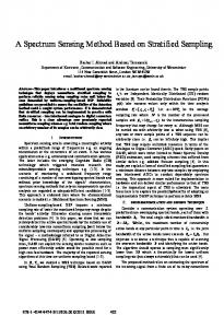
curves in Figure 1 is based on the combined stratified samples. On the other hand, the ones given by the dashed lines represent the density estimates for each stratum, namely based on male and female newborns. Note that, the densities of TSB levels for male and female newborns are not completely overlapping, which suggests the importance of stratified sampling in this case. Our findings show that using SRSS is more efficient for estimating the kernel densities. It can easily capture the shape of the strata densities into the overall density. However, under the SRS the estimated densities are less smooth. Hence, SRSS provides better representative sampling design. Hence SRSS is more robust than SSRS for representing the population for KDE.

7. Discussion This paper studies the KDE technique based on stratified ranked set and SRS and investigates their relative performance. We study the properties of the proposed estimates and give expressions for their bias and variance. The KDEs under both sampling techniques are found to be asymptotically unbiased. However, the SRSS results in smaller mean square error, in estimating densities through kernel, as compared with SSRS. In case of SRSS, for a fixed set size rh , an optimal choice of cycle sizes M = {mh : h = 1, 2, . . . , L} are given by minimizing the Table . Sampled data showing the weight at birth (X) and bilirubin level (Y) for both SRSS and SSRS. Females Cycle

Males

Weight (X) (kg)

TSB (Y) (Mg/dl)

Weight (X) (kg)

TSB (Y) (mg/dl)



. . . .

. . . .



. . . .

. . . .

. . . . . . . . . . . .

. . . . . . . . . . . .

. . . . . . . . . . . .

. . . . . . . . . . . .

SRSS 

. . . .

. . . .



. . . .

. . . .



17

Figure . Kernel density estimate for TSB at birth in newborn babies based on all population, SRSS and SSRS. The three density estimates are obtained one for each stratum (males and females) and the overall sample as well.

variance at a specified sampling cost. Later, the optimal allocation is extended for unbalanced case. Simulation studies are designed under varying distributional assumptions to compare the efficiency of the kernel density estimates under SRSS relative to SSRS. Although the estimated biases under both sampling schemes are found to be negligible, the positive values of relative improvement mean integrated squared errors (RMISE) imply that SRSS is more efficient than SSRS. Moreover, the near-optimal allocation presented in the simulation study shows more improvement in the RMISE when using SRSS.

Acknowledgments The authors thank the associate editor and the reviewers for their important and valuable comments and suggestions which improved the manuscript.

References Alexandre, B.T. (2009). Introduction to Nonparametric Estimation. New York, NY: Springer-Verlag. Baxter, M.J., Beardah, C.C., Westwood, S. (2000). Sample size and related issues in the analysis of lead isotope data. J. Archaeological Sci. 27:973–980.


18

H. SAMAWI ET AL.

Bellhouse, D.R., Stafford, J.E. (1999). Density estimation from complex surveys. Statistical Sinica. 9:407– 424. Bowman, A.W., Azzalini, A. (1997). Applied Smoothing Techniques for Data Analysis: The Kernel Approach with S-Plus Illustrations. Oxford, UK: Oxford University Press. Breunig, R. (2008). Nonparametric density estimation for stratified samples. Stat Probabil Lett. 78(14):2194–2200. Chen, Z. (1999). Density estimation using ranked-set sampling data. Environ Ecol Stat. 6:135–146. Chen, Z.H., Sinha, B.K., Bai, Z. (2004). Ranked Set Sampling: Theory and Applications. New York, NY: Springer. Dinardo, J., Fortin, N.M., Lemieux, T. (1996). Labor market institutions and the distribution of wages, 1973–1992: A semiparametric approach. Econometrica. 64:1001–1044. Ferreyra, R.A., Podesta, G.P., Messina, C.D., Letson, D., Dardanelli, J., Guevara, E., Meira, S. (2001). A linked-modeling framework to estimate maize production risk associated with ENSO-related climate variability in Argentina. Agr. Forest. Meteorol. 107:177–192. Fix, E., Hodges, J. (1951). Discriminatory Analysis, Nonparametric Discrimination: Consistency Properties. Technical Report No. 4. Project No. 21–29-004. Randolph Field, TX: USAF School of Aviation Medicine. Jeffrey, S.S. (1996). Smoothing Methods in Statistics. New York, NY: Springer-Verlag. Kaur, A., Patil, G.P., Sinha, A.K., Tailie, C. (1995). Ranked set sampling: An annotated bibliography. Environ Ecol Stat. 2:25–54. Kim, K.D., Heo, J.-H. (2002). Comparative study of flood quantiles estimation by nonparametric models. J. Hydrology. 260:176–193. Lim, J., Chen, M., Park, S., Wang, X., Stokes, L. (2014). Kernel density estimator from ranked set samples. Commun Stat Theory Meth. 43:2156–2168. McIntyre, G.A. (1952). A method for unbiased selective sampling using ranked set. Aus J Agricul Res. 3:385–390. Nazari, S., Jozani, M.J., Kharrati-Kopaei, M. (2014). Nonparametric density estimation using partially rank-ordered set samples with application in estimating the distribution of wheat yield. Electron J Stat. 8:738–761. Patil, G.P., Sinha, A.K., Taillie, C. (1999). Ranked set sampling: A bibliography. Environ Ecol Stat. 6:91– 98. Paulsen, O., Heggelund, P. (1996). Quantal properties of spontaneous EPSCs in neurons of the Guineapig dorsal lateralgeniculate nucleus. J. Physiology. 496:759–772. Rosenblatt, M. (1971). Curve estimates. Ann. Math. Stat. 42:1815–1842. Samawi, H.M. (1996). Stratified ranked set sample. Pakistan J Stat. 12(1):9–16. Samawi, H.M., Al-Sakeer, O.A.M. (2001). On the estimation of the distribution function using extreme and median ranked set sampling. Biometrical J. 43:357–373. Segal, M.R., Wiemels, J.L. (2002). Clustering of translocation break points. J. Amer. Statist. Assoc. 97:66– 76. Simonoff, J.S. (1996). Smoothing Methods in Statistics. New York, NY: Springer. Silverman, B.W. (1986). Density Estimation for Statistics and Data Analysis. London, UK: Chapman and Hall. Singh, R.S. (1977). Applications of estimators of a density and its derivatives. J Royal Stat Soc B. 39(3):357–363. Takahasi, K., Wakimoto, K. (1968). On unbiased estimates of the population mean based on the stratified sampling by means of ordering. Ann. Inst. Statist. Math. 20:1–31. Tortosa-Ausina, E. (2002). Financial costs, operating costs, and specialization of Spanish banking firms as distribution dynamics. Appl Econ. 34:2165–2176. Wand, M.P., Jones, M.C. (1995). Kernel Smoothing. London, UK: Chapman and Hall. Wolfgang, H., Marlene, M., Stefan, S., Axel, W. (2004). Nonparametric and Semiparametric Models. Berlin, Heidelberg, Germany: Springer-Verlag.