{ dalang, klaas, nando }@cs.ubc.ca. Dept. of Computer Science. University of British Columbia. Vancouver, BC, Canada V6T1Z4. Nando de Freitas. Abstract.
Insights on Fast Kernel Density Estimation Algorithms
Dustin Lang
Mike Klaas { dalang, klaas, nando }@cs.ubc.ca Dept. of Computer Science University of British Columbia Vancouver, BC, Canada V6T1Z4
Abstract
For simplicity, we consider a subset of the KDE problem in this paper. Some of these simplifying assumptions can be easily relaxed for some of the fast methods, but we assume that these will not change the essential properties that we examine. Specifically, we assume: ! 2 kxi − yj k Ki (xi , yj ) = exp − h2
We present results of experiments testing the Fast Gauss Transform, Improved Fast Gauss Transform, and Dual-Tree methods (using kd-tree and Anchors Hierarchy data structures) for fast Kernel Density Estimation (KDE). We examine the performance of these methods with respect to data set size, dimension, allowable error, and data set structure (“clumpiness”), measured in terms of CPU time and memory usage. This is the first multi-method comparison in the literature. The results are striking, challenging several claims that are commonly made about these methods. The results will be useful for researchers considering fast methods for KDE problems. We also provide theoretical results that improve the bounds on dual tree methods.
1
wi ≥ 0 M =N . That is, we consider the points to live in a vector space, and use a Gaussian kernel, non-negative weights, and equal numbers of sources and targets. To be useful to a broad audience, we feel that fast KDE methods must allow the user to set a guaranteed absolute error level. That is, given an allowable error �, the method must return approximations fˆj such that ˆ fj − fj ≤ � .
INTRODUCTION
This paper examines several methods for speeding up KDE. This problem arises as a basic operation in many statistical settings, including message passing in belief propagation, particle smoothing, population Monte Carlo, spectral clustering, SVMs and Gaussian processes.
fj =
wi Ki (xi , yj ) ,
j = 1...M .
Ideally, the methods should work well even with small �, so that one can simply “plug it in and forget about it.”
2
(1)
i=1
The points X = {xi } , i = 1 . . . N each have a weight wi . We call these source particles. We call the points Y = {yj } , j = 1 . . . M the target points. We call fj the influence at point yj , and K is the kernel function.
FAST METHODS
In this section, we briefly summarize each of the methods that we test. 2.1
The KDE problem is to compute the values N X
Nando de Freitas
Fast Gauss Transform
The Fast Gauss Transform (FGT) was introduced by Greengard and Strain [5, 6, 2]. It is a specialization of the Fast Multipole Method to the particular properties of the Gaussian kernel. The algorithm begins by dividing the space into boxes and assigning sources and targets to boxes. For the source boxes, Hermite series expansion coefficients are computed. Since the Gaussian falls off quickly, only a limited number of source
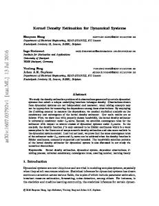
PSfrag replacements dy rx
xB
The error bound given is equation 3.13 in [9]: � � ry 2 , EC ≤ W exp − 2 h
d
x
y
Cluster B
Figure 1: An illustration of the IFGT error bound due to ignoring clusters outside radius ry . The cluster center is xB and its radius is rx ; the cluster is ignored if the distance dy from the center to y is greater than ry . In the worst case, a particle x with large weight sits on the cluster boundary nearest to y. The distance dy is slightly larger than ry , so the cluster is ignored. The distance between y and x can be as small as d = ry −rx , not ry . boxes will have non-negligible influence upon a given target box. These neighbouring boxes are collected, and the Hermite expansions are combined to form a Taylor expansion that is valid inside the target box. The FGT implementation we test was graciously provided by Firas Hamze, and is written in C with a Matlab wrapper. It uses a fairly simple space-subdivision � � � 3 . scheme, so has memory requirements of O h1 Adaptive space subdivision or sparse memory allocation could perhaps improve the performance, particularly for small-bandwidth problems. 2.2
Improved Fast Gauss Transform
The Improved Fast Gauss Transform (IFGT) [9, 10] aims to improve upon the FGT by using a space partitioning scheme and series expansion that scale better with dimension. The space-partitioning scheme is the farthest-point Kcenters algorithm, which performs a simple clustering of the source particles into K clusters. As in the FGT, the series expansion coefficients for the source points in each cluster can be summed. The IFGT does not build a space-partitioning tree for the target points. Rather, for each target point it finds the set of source clusters that are within range, and evaluates the series expansion for each. The implementation of the IFGT that we test was generously provided by Changjiang Yang and Ramani Duraiswami. It is written in C++ with Matlab bindings. 2.2.1
IFGT Error Bounds
The original IFGT papers contain an incorrect error bound, which we correct here.
where W is the sum of source weights. This is the error that results from ignoring the influence of source clusters that are outside of range ry from a target point. That is, if the center of cluster B is xB , then the influence of the cluster on target point y is ignored if the distance kxB − yj k > ry . This bound is incorrect, as illustrated in Figure 1. The correct bound is � � (ry − rx ) 2 . EC ≤ W exp − h2 2.2.2
Choosing IFGT Parameters
The IFGT has several parameters that must be chosen, yet the original papers ([10, 9]) do not suggest a method for choosing these parameters. We developed a protocol for automatically choosing parameters that will satisfy a given error bound �, without seriously degrading the computational complexity of the algorithm. We make no claim that this protocol is optimal. The parameters that must be chosen include K, the number of source clusters; p, the number of terms in the series expansion; and ry , the range. As K increases, the radius of the largest source cluster, rx , decreases. The IFGT has two sources of error. The first is discussed above, and is due to ignoring clusters that are outside range ry from a given target point. The second is due to truncation of the series expansion after order p. This is called ET in equation 3.12 of [9]: � � 2 r x r y − r x 2 − r y 2 2p � r x r y � p ET ≤ W exp h2 p! h2 where rx is the maximum source cluster radius, ry is the range, and p is the order of the series expansion. See Figure 2 for the protocol. It is based on four constraints C: C1 : EC C2 : ET C3 : � K rx r y � C4 : h2
≤ � ≤ � ≤ K∗ ≤ 1
where C1 and C2 are hard constraints that guarantee the error bound, C3 is a hard constraint that guarantees the algorithmic complexity, and C4 is a soft constraint that improves convergence. Note that each source cluster contributes to the error either through series expansion (ET ) or by being ignored (EC ), but not both, so it suffices to require EC ≤ � and ET ≤ �.
Input: ry (ideal), � Output: k, ry , p Algorithm: for k = 1 to K ∗ : run k-centers algorithm. find largest cluster radius rx . using ry = ry (ideal), compute C1 , C4 . if C1 and C4 : break if k < K ∗ : // C4 can be satisfied. set ry = min(ry ) such that C1 and C4 . else: // C4 cannot be satisfied. set ry = min(ry ) such that C1 . set p = min(p) such that C2 . Figure 2: Protocol for choosing IFGT parameters. We first try to find k < K ∗ that will allow all the constraints to be satisfied with the given ry (ideal). In many cases, this is not possible so we must set k = K ∗ and increase ry . Finally, we choose p to satisfy the truncation error bound C2 . In practice, the k-centers algorithm is run iteratively rather than being run anew each time through the loop. Note that the IFGT, unlike the FGT, does not cluster the target points y; the distance from each target to each source cluster is computed. The algorithm therefore has O (KM ) complexity, where K is the number of source clusters and M is the number of targets. To keep O (M ) complexity, K must be bounded above by a constant, K ∗ . This is constraint C3 . Note that rx (the maximum cluster radius) decreases as K (the number of clusters) increases. Since K has an upper bound, rx has a lower bound. Contrary to the claim in [9], rx cannot be made as small as required by increasing K while still maintaining O (M ) complexity. 2.3
DUAL-TREE
We developed an implementation of the dual-tree recursion described by Gray and Moore [4, 3]. We make several implementation-level changes, as detailed in [7]. The dual-tree strategy is based on building spacepartitioning trees for both the source and target points. The algorithm proceeds by expanding the ‘cross product’ of the trees in such a way that only areas of the trees that contain useful information are explored. With these trees, it is inexpensive to compute distance bounds between nodes, which allows us to bound the influence of a source node upon a target node. If the influence bound is too loose, it can be tightened by expanding the nodes; that is, by replacing
the parent nodes with the sum of their children. When the influence bounds have been tightened sufficiently (below �), we are finished. A major difference between the dual-tree strategy and the series expansion-based methods (FGT and IFGT) is that the expansion-based methods guarantee error bounds based on theoretical bounds on the series truncation error. These bounds are computed a priori, and are valid for all data distributions. However, since they are based on worst-case behaviour, they are often quite loose for average-case problems. Conversely, the dual-tree strategy is based solely on error bounds determined at run time, so is fundamentally concerned with a particular data set. Our implementation of the dual-tree strategy is independent of the space-partitioning strategy. We implemented the classic kd-tree and the Anchors Hierarchy [8]. It is written in C with Matlab bindings.
3
RESULTS
All tests were run on our Xeon 2.4 GHz, 1 GB memory, compute servers. We ran the tests within Matlab; all the fast algorithms are written in C or C++ and have Matlab bindings. We stopped testing a method once its memory requirements rose above 1 GB in order to avoid swapping. In all cases we repeated the tests with several data sets. In some of the plots the error bars are omitted for clarity. The error bars are typically very small. Most of the plots have log-log scales. For the IFGT, we set the √ upper bound on the number of clusters to be K ∗ = N . In practice, K ∗ should be set to a constant, but since we are testing over several orders of magnitude this seems more reasonable. The curves labelled “KDtree” and “Anchors” are our dual-tree implementation using kd-tree and Anchors Hierarchy space-partitioning trees. “Naive” is the � straightforward O N 2 summation. Many of the tests below can be seen as onedimensional probes in parameter space about the point N = 10, 000, Gaussian bandwidth h = 0.01, dimension D = 3, allowable error � = 10−6 , clumpiness C = 1 (ie, uniform) point distribution, with weights drawn uniformly from [0, 1]. In all cases the points are confined to the unit D-cube. We occasionally choose other parameters in order to illustrate a particular point. We use D = 3 to allow the FGT to be tested. 3.1
Test A: N
Researchers have focused attention on the performance of fast algorithms with respect to N (the number of source and target points). Figure 3 shows that it is crucially important to consider other factors, since these
required is more than 1010 for N = 100. The dual-tree methods perform well, though memory usage is still a concern.
strongly influence the empirical performance. 4
10
2
10 10
1
CPU Time (s)
CPU Time (s)
2
0
10
Naive FGT IFGT Anchors KDtree
−2
10
2
10
3
10
4
N
10
10
0
10
−1
Naive FGT Anchors KDtree
10 5
10
−2
10
2
10
9
10
3
10
4
10 N
5
10
8
10
Memory Usage (bytes)
Memory Usage (bytes)
9
10
7
10
FGT IFGT Anchors KDtree
6
10
2
10
3
10
4
N
10
8
10
7
10
FGT Anchors KDtree
6
5
10
10
2
Figure 3: Test A: D = 3, h = 0.1, uniform data, � = 10−6 . In this test, the scale of the Gaussians is h = 0.1, so a large proportion of the space has a significant contribution to the total influence. An important observation in Figure 3 is that the dual-tree methods (KDtree � and Anchors) are doing about O N 2 work. Empirically, they are never faster than Naive for this problem. Indeed, only the FGT is ever faster, and then only for a small range of N . The IFGT appears to be demonstrating better asymptotic performance, but the crossover point (if the trend continues) occurs at about 1.5 hours of compute time. Another important thing to note in Figure 3 is that the dual-tree methods run out of memory before reaching N = 50, 000 points; this happens after a modest amount of compute time. Also of interest is the fact that the IFGT has decreasing memory requirements. We presume this is because the number of clusters increases, so the cluster radii decrease and the error bounds converge toward zero more quickly, meaning that fewer expansion terms are required. 3.2
Test B: N
In this test, we repeat test A but use a smaller Gaussian scale parameter, h = 0.01. The behaviour of the algorithms is strikingly different. We can no longer run the IFGT, since the number of expansion terms
10
3
10
4
N
10
5
10
Figure 4: Test B: D = 3, h = 0.01, uniform data, � = 10−6 . 3.3
Test C: Dimension D
In this test, we fix N = 10, 000 and vary the dimension. We set � = 10−3 to allow the IFGT to run in a reasonable amount of time. Surprisingly, the IFGT and Anchors, both of which are supposed to work well in high dimension, do not perform particularly well. The IFGT’s computational requirements become infeasibly large above D = 2, while Anchors never does better than KDtree. This continues to be true even when we subtract the time required to build the Anchors Hierarchy. 3.4
Test D: Allowable Error �
In this test, we examine the cost of decreasing �. The dual-tree methods have slowly-increasing costs as the accuracy is increased. The FGT has a more quickly increasing cost, but for this problem it is still competitive at � = 10−11 . We find that the dual-tree methods begin to have problems when � < 10−11 ; while these methods can give arbitrarily accurate approximations given exact arithmetic, in practice they are prone to cancellation error. The bottom plot in Figure 6 shows the maximum error
3.5
DATA SET CLUMPINESS
3
CPU Time (s)
10
Next, we explore the behaviour of the fast methods on data sets drawn from non-uniform distributions.
2
10
1
10
Naive FGT IFGT Anchors KDtree
0
10
−1
10
0
1
10
2
10 Dimension
10
Figure 5: Test C: h = 0.01, � = 10−3 , N = 10, 000, uniform data.
in the estimates. The dual-tree methods produce results whose maximum errors are almost exactly equal to the error tolerance �. One way of interpreting this is that these methods do as little work as possible to produce an estimate that satisfies the required bounds. The FGT, on the other hand, produces results that have real error well below the requirements. Notice the ‘steps’; we believe these occur as the algorithm either adds terms to the series expansion, or chooses to increase the number of boxes that are considered to be within range.
Naive FGT Anchors KDtree
We use a method for generating clumpy data that draws on the concept of lacunarity. Lacunarity [1] measures the texture or ‘difference from uniformity’ of a set of points, and is distinct from fractal dimension. It is a scale-dependent quantity that measures the width of the distribution of point density. Lacunarity at a given scale can be measured by covering the set with boxes of that scale; the distribution of point densities in the boxes is measured, and the lacunarity is defined as the second moment of the distribution divided by the first moment squared.
Figure 7: Example clumpy data sets. The clumpinesses are C = 1 (left), C = 1.5 (middle), and C = 3 (right). Each data set contains 1000 points. We adapt the notion of the ratio of variance to squared mean. Given a number of samples N and a clumpiness C, our clumpy data generator recursively divides the space into 2D sub-boxes, and distributes the N samples among the sub-boxes such than D
2 X
CPU Time
1
10
Ni = N
i=1
var ({Ni }) = (C − 1) mean {Ni } 0
10
−1
10
−3
10
−5
10
−7
10 Epsilon
−9
−11
10
10
−5
Real Error
10
−10
10
−5
10
Epsilon
−10
10
Figure 6: Test D: D = 3, h = 0.01, N = 10, 000, uniform data. Top: CPU Time. Bottom: Real error.
.
This process continues until N is below some threshold (we use 10). Some example clumpy data sets are shown in Figure 7. 3.6
FGT Anchors KDtree
�2
Test E: Source Clumpiness
In this test, we draw the source particles X from a clumpy distribution, while the targets are drawn from a uniform distribution. Figure 8 shows the relative CPU time as clumpiness increases. The dual-tree methods show significant improvements as the source points become clumpy. Anchors improves more than KDtree, although KDtree is still faster in absolute terms. The FGT shows minor improvement as clumpiness increases. 3.7
Test F: Source and Target Clumpiness
In this test, we draw both the sources and targets from clumpy distributions. The dual-tree methods
2
10
0.9 CPU Time (s)
CPU Usage Relative to Uniform Data
1
0.8 0.7 0.6
0
10
Naive FGT Anchors KDtree
0.5 1
1.5
2 Data Clumpiness
2.5
show even more marked improvement as clumpiness increases. The FGT also shows greater improvement than in the previous test. CPU Usage Relative to Uniform Data
1
10
Dimension
weights sum to α0 , and they are between d(min) and d(max) in distance from y. We wish to bound the influence of X on y given by: fy (X) =
nX X
wi K(xi , y)
(4.2)
i=1
0.9
where nX is the number of particles in X. We assume K(·) is parameterized by a distance function, ie., K(x, y) , K (d(x, y)), and is monotonic in d(·).
0.8 0.7 0.6
4.2
0.5 0.4
Naive FGT Anchors KDtree
0.3 1
1.5
2 Data Clumpiness
2.5
3
Figure 9: Test F results: D = 3, h = 0.01, � = 10−6 , N = 10, 000, clumpy X, clumpy Y ; relative CPU time. Test G: Clumpy Data, Dimension D
In this test, we test the performance with dimension, given clumpy data sets. The results are not very different than the uniform case (Test C). This is surprising, since neither Anchors nor IFGT does particularly well, even given clumpy data.
BETTER BOUNDS FOR DUAL-TREE METHODS
Current method
In existing dual-tree algorithms, we upperbound the influence as follows: � � fy (X) ≤ α0 · K d(min) (4.3) It is clear that this is an extremely pessimistic bound, as it is improbable that all the mass in X lies at the closest point to y. To improve this bound, we can consider the distribution of points within X. For instance, if we knew the centre of mass, we could rule out the worst case where all the mass was maximally close to y. The more constraints we add, the more information we have at our disposal about the distribution of the points, and consequently the tighter bounds we should be able to derive. A natural set of statistics to consider are the raw moments of the distribution. The nth raw moment is defined by αn =
We present some preliminary theoretical results that enable us to tighten the influence bounds that are at the heart of the dual-tree method. 4.1
10
Figure 10: Test G results: h = 0.01, � = 10−3 , N = 10, 000, clumpy X, clumpy Y .
1
4
Naive IFGT Anchors KDtree 0
3
Figure 8: Test E: D = 3, h = 0.01, � = 10−6 , N = 10, 000, clumpy X, uniform Y , relative CPU time.
3.8
1
10
Definitions
Consider a target point y and a node X in a spatial index. We denote by d(min) and d(max) the lower and upper bounds on the distance from y to any point in X. We know something about the points in X: their
nX X
wi xni
(4.4)
i=1
A cursory glance at equation (4.4) shows that we are already looking at moments: the first moment is the centre of mass of the points, and the zeroth moment corresponds to the constraint that the sum of mass in X is α0 . Our problem is as follows: given the first n moments of the distribution of the points in X, what is the maximum possible influence on y? We have already seen
the answer for n = 0, and we will shed some light on the solution for n ≥ 1. 4.3
Conjecture 4.3. The maximal solution to (4.5) can be written as a sum of two Dirac delta functions: w∗ (x) = w1 δ(x − x1 ) + w2 δ(x − x2 ) .
Continuous weight distribution
We proceed by defining w(x) to be a positive distribution of weight over points in X. The influence can then be written as the integral Z Fy (X) = K(x, y)w(x)dx (4.5) X
and we are interested in finding the maximum and minimum values this quantity can attain, subject to the moment constraints Z xi w(x)dx = αi , i = 0, . . . , n . (4.6)
We refer to this as a two-particle solution. Conjecture 4.4. For space-partitioning trees with spherical nodes and monotonic decreasing kernels, the point in Y that leads to the upper bound is the point nearest to the centre of X; the point that leads to the lower bound is the furthest point in Y . Call these points yn and yf , respectively. Theorem 4.5. For space-partitioning trees with spherical nodes, and where the centre of node X is the center of mass, the maximal two-particle solution has both particles positioned on the line connecting the centres of nodes X and Y .
X
This is an infinite linear programming problem. Assume w(x) is continuous. We set up a Lagrangian with multipliers Θ = {θ0 , . . . , θn }: L(w, Θ) = Fy (X) −
n X i=0
�Z
i
x w(x)dx − αi
θi
� (4.7)
X
Theorem 4.1. Given the optimization problem defined in (4.7) and n moment constraints, the existence of a continuous optimum w(x) implies that ∂ n+1 K(x, y) =0 . ∂xn+1 Proof. Differentiating the Lagrangian (4.7) by w(x) and setting to zero yields ! n X IX K(x, y) = IX θi xi , (4.8) i=0
where IX is the set membership function. Hence, K(x, y) is a polynomial of degree ≤ n when x ∈ X. Corollary 4.2. Given a finite set of moment constraints, the worst-case distribution for the maximum influence for a Gaussian kernel is given by a finite sum of Dirac masses. Proof. Assume n moment contraints are given. By Theorem 4.1, a continuous weight distribution implies ∂ n+1 K(x, y) = 0. But the Gaussian kernel is infinitely ∂xn+1 differentiable, and the derivative is always greater than zero: a contradiction. We now consider the Gaussian kernel and make the following conjectures.
Sketch of Proof. First, note that we can consider the two-dimensional plane that contains the axis (connecting the centres of X and Y ) and the two particles. Consider a rotation of the particles rigidly about their centre of mass. This preserves all the moments but changes the influence. It can be shown that the maximum influence is achieved when the particles lie on the axis. Conjecture 4.6. Given�the conditions of Theorem 4.5 and h ≤ √12 d(min) − R and d(min) > R, where R is the radius of cluster X, h is the scale of the Gaussian kernel, and d(min) is the minimum distance from the center of cluster X to Y , then the maximal two-particle solution has one particle on the radius: x1 = R. The upper influence bound can then be written in closed form. First, note that the moment constraints allow us to write w1 , w2 , and x2 in terms of x1 . Theorem 4.5 tells us that we need only consider the solution where x1 lies on the axis. We are thus left with a one-dimensional, one-variable optimization on a closed domain. We can solve this numerically, but this is rather expensive. For some combinations of R, d(min) , and h, it can be shown that the maximum occurs at the endpoint x1 = R. It is difficult to determine an exact closed-form expression for this region, however. Our numerical experiments suggest that the bound given above is correct, but we have thus far been unable to show it analytically. Conjecture 4.7. The minimal solution to (4.2) lies on the radius of a circle centered at the point yf . The radius of this circle can be written in closed form, and the minimum influence bound can be written in closed form. Sketch of Proof. We can show that the minimal solution for the two-particle solution (in two dimensions)
lies on the radius of this circle by taking derivatives of the influence function and solving the simultaneous equations that result. This allows us to find the radius of the circle on which the particles must lie; the closed form of the minimum influence bound follows. Since the solution for the two-particle case is a curve rather than a point, we suspect that it is not only the solution to the two-particle case but also the general case. 4.4
Experiments
We ran our dual-tree algorithm with the Anchors Hierarchy, computing at each step both the standard bounds (4.3) and the better bounds described in the conjectures above. We find that the better upper bound is at most half as large as the original bound. The find that the better lower bound is considerable larger than the original bound. See Figure 11. 4500
well when there is structure in the kernel matrix. They also indicate that dual tree methods are preferable in high dimensions. Surprisingly, the results show that the KDtree works better than the Anchors Hierarchy in our particular experiments. This seems to contradict common beliefs about these methods. Yet, there is a lack of methodological comparisons between these methods in the literature. This makes it clear that further investigation is warranted. We presented theoretical results that enable us to tighten the bounds on dual-tree methods. Some of the results are general. Others require assumptions on the type of kernel as well as some intuitive conjectures that remain to be proved. The new bounds are always equal to or tighter than the original bounds, and have almost no extra computational cost. This should allow the dual-tree method to run more quickly, since fewer nodes will need to be expanded.
References
4000
[1] C Allain and M Cloitre. Characterizing the lacunarity of random and deterministic fractal sets. Physical Review A, 44(6):3552–3558, Sep 1991.
3500
Counts
3000 2500
[2] B J C Baxter and G Roussos. A new error estimate of the fast Gauss transform. SIAM Journal of Scientific Computing, 24(1):257–259, 2002.
2000 1500 1000
[3] A Gray and A Moore. Nonparametric density estimation: Toward computational tractability. In SIAM International Conference on Data Mining, 2003.
500 0
1/16
1/8
1/4 Better / Original
1/2
1
900 800
[5] L Greengard and J Strain. The fast Gauss transform. SIAM Journal of Scientific Statistical Computing, 12(1):79–94, 1991.
700 600 Counts
[4] A G Gray and A W Moore. ‘N-Body’ problems in statistical learning. In NIPS 4, pages 521–527, 2000.
[6] L Greengard and X Sun. A new version of the Fast gauss transform. Documenta Mathematica, ICM(3):575–584, 1998.
500 400 300
[7] D Lang. Fast methods for inference in graphical models. Master’s thesis, University of British Columbia, 2004.
200 100 0 1
10^50
10^100 10^150 Original / Better
10^200
Figure 11: Better bounds results. Top: Upper bound. Bottom: Lower bound.
5
CONCLUSIONS
We presented the first comparison between the most widely used fast methods for KDE. In our comparison, we varied not only the number of interacting points N , but also the structure in the data, the required precision and the dimension of the state space. The results indicate that the fast methods can only work
[8] A Moore. The Anchors Hierarchy: Using the triangle inequality to survive high dimensional data. Technical Report CMU-RI-TR-00-05, Carnegie Mellon University, February 2000. [9] C Yang, R Duraiswami, and N A Gumerov. Improved fast gauss transform. Technical Report CS–TR–4495, University of Maryland, 2003. [10] C Yang, R Duraiswami, N A Gumerov, and L S Davis. Improved fast Gauss transform and efficient kernel density estimation. In ICCV, Nice, 2003.