Feb 2, 2008 - graphs can be derived from the free energy of the q-state Potts model ... the Potts free energy with respect to ln q is related to the component.
arXiv:cond-mat/0311535v2 [cond-mat.stat-mech] 21 Jan 2004
On large deviation properties of Erd¨os-R´enyi random graphs Andreas Engel1,2 , R´emi Monasson2,3 , and Alexander K. Hartmann4 1 Institut f¨ ur Physik, Universit¨at Oldenburg, 26111 Oldenburg, Germany. 2 CNRS-Laboratoire de Physique Th´eorique, 3 rue de l’Universit´e, 67000 Strasbourg, France. 3 CNRS-Laboratoire de Physique Th´eorique de l’ENS, 24 rue Lhomond, 75005 Paris, France. 4 Institut f¨ ur Theoretische Physik, Tammannstraße 1, 37077 G¨ottingen, Germany February 2, 2008 Abstract We show that large deviation properties of Erd¨ os-R´enyi random graphs can be derived from the free energy of the q-state Potts model of statistical mechanics. More precisely the Legendre transform of the Potts free energy with respect to ln q is related to the component generating function of the graph ensemble. This generalizes the wellknown mapping between typical properties of random graphs and the q → 1 limit of the Potts free energy. For exponentially rare graphs we explicitly calculate the number of components, the size of the giant component, the degree distributions inside and outside the giant component, and the distribution of small component sizes. We also perform numerical simulations which are in very good agreement with our analytical work. Finally we demonstrate how the same results can be derived by studying the evolution of random graphs under the insertion of new vertices and edges, without recourse to the thermodynamics of the Potts model.
PACS: 02.50.-r, 05.50.+q, 75.10.Nr
1
Introduction
Random graphs have kept being an issue of tremendous interest in probability and graph theory ever since the seminal work by Erd¨ os and R´enyi [1] 1
more than four decades ago. In addition to fixed edge number and fixed edge probability distributions also random graphs with constant vertex degree [2] or power law degree distribution [3, 4] have been investigated. Most of the efforts devoted to the study of the properties of random graphs have taken advantage of the fact that these properties undergo some concentration process in the infinite size (number of vertices) limit. For instance, the numbers of vertices in the largest component or the number of connected components, which are stochastic in nature, become highly concentrated in this limit, and with high probability do not differ from their average values. For large but finite sizes, properties as the one evoked above obviously fluctuate from graph to graph. The understanding of their statistical deviations are important for several problems in statistical physics, e.g. for the life-time of metastable states and the extremal properties of models defined on random graphs [5], as well as in computer science, e.g. for information-packet transmission in random networks [6, 7], resolution of random decision problems with search procedures [8, 9, 10] and others. Up to now apparently little attention has been paid to a quantitative characterization of large deviations in random graph ensembles [11, 12]. The present work is intended to contribute to an improved understanding of rare fluctuations in random graphs. Our main objective was to devise a microscopic ”mean-field” approach permitting to handle such rare deviations in much the same way as for average properties of various similar problems, as e.g. bootstrap and rigidity percolation [13] and spin-glasses [14]. The mean-field approach relies on a statistical stability argument: a large graph is not strongly modified when adding an edge and/or a vertex. This statement can be translated into some self-consistent equations for the average value of physical properties of interest, as e.g. the magnetization for a spin system, or the probability of belonging to the k-core for bootstrap percolation. We will show in the present work that a similar self-consistent approach can also be successfully used to access large deviations in random graphs. The main property we focus on throughout this paper is the number of connected components of a random graph. As established by Fortuin and Kasteleyn [15], several properties of random graphs with a typical number of components can be inferred from the knowledge of the thermodynamics of the q-state Potts model on a complete graph for values of q around 1. We will show that the thermodynamic properties for general values of q can be used to additionally characterize the properties of random graphs with an atypical number of components. This allows us to verify the validity of our microscopic mean-field approach. This paper is organized as follows. In Section 2, we introduce the basic definitions and notations for the quantities studied. Section 3 is devoted to the derivation of rare graphs properties through the study of the Potts 2
model. We show in Section 4 how these results can be rederived through the requirement of the statistical stability of very large atypical graphs against the addition of a vertex and its attached edges, or an edge. In Section 5 we describe our numerical procedure to simulate large deviation properties of random graphs ensembles. Some conclusion is finally proposed in Section 6.
2
Basic notions
We begin by fixing some vocabulary. For a detailed and precise account on random graphs we refer the reader to the textbook [16]. A graph G is a collection of vertices numbered by i = 1, . . . , N with edges (i, j), i 6= j, i, j = 1, . . . , N connecting them. The number of edges is between 0 (for the empty graph) and N (N − 1)/2 (for the complete graph). A component of a graph is a subset of connected vertices which are disconnect from the rest of the graph. The size S of a component is the number of vertices it contains. Hence the empty graph consists of N components of size 1 whereas the complete graph is made from a single component of size N . The number of components of a graph G is denoted by C(G). We are generally interested in properties of large graphs, N → ∞. We will consider random graphs in the sense that an edge between two vertices may be present or absent with a certain probability. The various joint probabilities to be discussed below will be denoted in the form P (x1 , x2 , ...; a1 , a2 , ...) with the xi representing the random variables and the ai denoting the parameters of the distribution. In particular we consider random graphs in which each pair of vertices is connected by an edge with probability γ/N independently of all other pairs of vertices. The parameter γ characterizes the connectivity of the graph. Since each vertex establishes edges with probability γ/N with all the other N − 1 vertices γ is in the limit N → ∞ just the typical degree of a vertex denoted by d∗ , giving the average number of edges emanating from it. More precisely, in this limit the degree d of a vertex is a random variable obeying a Poisson law with parameter γ, P (d; γ) = e−γ
γd . d!
(1)
In particular, P (d = 0; γ) = e−γ is the fraction of isolated vertices. Hence the average number of components of a random graph of the described type is bounded from below by N e−γ . Note also that the typical degree d∗ of a vertex remains finite for N → ∞. Typical realization of such random graphs are therefore sparse. The probability P (G; γ, N ) of one particular random graph G with N
3
vertices and parameter γ derives from the binomial law, � γ �L(G) �
γ �( 2 )−L(G) N N � γ �L(G) L(G) γ 1 − γN +γ( − + 2 4 N )+o(1) , =e 2 N
P (G; γ, N ) =
N
1−
(2)
where L(G) = O(N ) denotes the number of edges of graph G. To describe the decomposition of a large random graph into its components, it is convenient to introduce the probability P (C; γ, N ) of a random graph with N vertices to have C components X P (C; γ, N ) = P (G; γ, N ) δ(C, C(G)), (3) G
where δ(a, b) denotes the Kronecker delta. A general observation is that for given γ and large N the probability P (C; γ, N ) gets sharply peaked at some typical value C ∗ of C and the probabilities for values of C significantly different from C ∗ being exponentially small in N . To describe this fact more quantitatively we introduce the number of components per vertex c = C/N together with the quantity ω(c, γ) = lim
N →∞
1 ln P (C; γ, N ). N
(4)
Clearly ω(c, γ) ≤ 0 and the typical value c∗ of c has ω(c∗ , γ) = 0. Averages with P (G; γ, N ) are therefore dominated by graphs with a typical number of components. The focus of the present paper is on properties of random graphs which are atypical with respect to their number of components C. In order to get access to the properties of these graphs we introduce the biased probability distributions P (G; γ, q, N ) =
1 P (G; γ, N ) q C(G) , Z(γ, q, N )
with Z(γ, q, N ) defined by X X Z(γ, q, N ) = P (G; γ, N ) q C(G) = P (C; γ, N ) q C . G
(5)
(6)
C
The normalization constant Z(γ, q, N ) in (5) has hence the meaning of a component generating function of P (G; γ, N ). Contrary to averages with P (G; γ, N ) those with P (G; γ, q, N ) are dominated by graphs with an atypical number of components which is fixed implicitly with the parameter q. Values of q smaller than 1 shift weight to graphs with few components 4
whereas for q > 1 graphs with many components dominate the distribution. The typical case is obviously recovered for q = 1. Similar to ω(c, γ) it is convenient to introduce the function ϕ(γ, q) = lim
N →∞
1 ln Z(γ, q, N ). N
From (6) and (4) it follows to leading order in N that Z 1 Z(γ, q, N ) = dc exp(N [ω(c, γ) + c ln q])
(7)
(8)
0
and performing the integral by the Laplace method for large N we find that ϕ(γ, q) and ω(c, γ) are Legendre transforms of each other: ϕ(γ, q) = max [ω(c, γ) + c ln q]
ω(c, γ) = min [ϕ(γ, q) − c ln q]
c
q = exp(−
q
∂ω ) ∂c
c=q
∂ϕ ∂q
(9) (10)
The large deviation properties of the ensemble of random graphs as characterized by ω(c, γ) can hence be inferred from ϕ(γ, q). In the next section we show how ϕ(γ, q) can be obtained from the statistical mechanics of the Potts model. For later use we also note that from differentiating (7) with respect to γ we find using (6) and (2) to leading order in N ℓ(γ, q) =
γ ∂ϕ +γ . 2 ∂γ
(11)
Here ℓ(γ, q) denotes the average number of edges per vertex in the graph where the average is performed with the distribution (5).
3 3.1
Thermodynamics of atypical graphs The mean-field Potts model
It has long been known [15] that certain characteristics of random graphs are related to the thermodynamic properties of the Potts model [17, 18]. The Potts model is defined in terms of an energy function E({σi }) depending on N spin variables σi , i = 1, . . . , N , which may take on q distinct values σ = 0, 1, ..., q −1. In the mean-field variant the energy function reads E({σi }) = −
q−1 X X 1 X δ(σ, σi ), uσ δ(σi , σj ) − h N i 0 branches off continuously from the high-temperature solution s0 = 0 at β = q. For q > 2 the new solution appears discontinuously at the spinodal point β s < q by a subcritical bifurcation.
where huσ is an auxiliary field parallel to the direction σ. The thermodynamic properties of the system at inverse temperature β can be derived from the partition function X exp(−βE({σi })) (13) Z(β, h, q, {uσ }, N ) = {σi }
where the sum runs over all q N spin configurations {σi }. A standard analysis (cf. the appendix) gives for the free energy 1 ln Z(β, h, q, {uσ }, N ) N →∞ βN
f (β, h, q, {uσ }) = − lim
(14)
at h = 0 the result � 1 q−1 2 1 f (β, q) = extr − − s − ln q s0 2q 2q 0 β � 1 + (q − 1)s0 q−1 + ln(1 + (q − 1)s0 ) + (1 − s0 ) ln(1 − s0 ) . (15) βq βq The saddle-point value s0 (β, q) extremizing the expression in the brackets is the stable solution of the equation eβs0 =
1 + (q − 1)s0 . 1 − s0 6
(16)
Clearly s0 = 0 is always a solution of this equation. It is, however, unstable for large β and another, non-trivial solution becomes stable which describes the spontaneous appearance of order in the low temperature phase. Fig. 1 displays the solutions of (16) as function of β for different values of q. Note the subcriticial bifurcation in s0 (β, q) for q > 2.
3.2
Diagrammatic expansion of the Potts model
The relation between the Potts model and the random graph ensemble introduced in section 2 becomes apparent when considering the hightemperature expansion of the free energy (14) of the Potts model. Since the Kronecker delta can take only the values zero or unity, the partition function (13) can be recast into the form [15] X Y P P [1 + w δ(σi , σj )] e β h σ uσ i δ(σi ,σ) , (17) Z(β, h, q, {uσ }, N ) = {σi } i 0. We have hence to study the extremization over s in (23) for fixed γ and variable q. This is somewhat complementary to what is done in the statistical mechanics of the Potts model where the free energy (15) is minimized for integer q ≥ 2 and different values of β. Here we have to keep in mind that the extremum in (23) is a minimum if q > 1 but a maximum if 0 < q < 11 . The dependence of ϕ(γ, q) on q is qualitatively different for γ ≤ 2 and γ > 2 as shown in Fig. 3. For γ ≤ 2 the stable solution of (24) is positive for q < γ, goes to zero for q → γ, and is identically zero for q > γ (cf. left inset in Fig. 3). Accordingly ϕ(γ, q) shows a second order phase transition at 1 The reason for this is that due to the constraint (120) the free energy depends on (q − 1) variables, a number which becomes negative for q < 1.
10
0.1
0.05 1
1
s0 0.5
s0 0.5
0 0
A
0
0.5
1
1.5
0
0.05
2
0
2
q
4
6
8
ϕ(q)
ϕ(q)
q
−0.05
B
A 0
B
D
−0.1
C 0.5
0.75
1
1.25
q
1.5
1.75
−0.05
2
1
2
3
4
q
5
6
7
Figure 3: Free energy (23) of the random graph ensemble as a function of q for connectivities γ = 1.8 (left) and γ = 4 (right). The full and dashed curve correspond to the small clusters phase (s0 = 0) and the giant component phase (s0 > 0) respectively. Both free energies coincide in q = 1 (point A). For γ ≤ 2 (left), a second order phase transition arises when q crosses q = γ (point B) with the size of the giant component approaching zero continuously (left inset). When γ > 2 (right), the transition takes place at point C with abscissa q M > γ and is first order. Both the slope of the free energy and the size of the giant component (right inset) are discontinuous at the transition. Branches BD and CD correspond to unstable (local maximum) and metastable (secondary local minimum) solutions respectively.
q = γ as displayed in the left part of Fig. 3. For γ > 2 the small-q solution s0 (γ, q) > 0 remains stable up to q = q s > γ and coexists for γ < q < q s with the solution s0 = 0 which is stable for q > γ as before, see right inset in Fig. 3. Accordingly the phase transition is now first order and takes place at the Maxwell point q = q M where the two values of ϕ(γ, q) coincide as shown in the right panel of Fig. 3. At the transition, the value of s0 jumps discontinuously, and so does the derivative of ϕ(γ, q) with respect to q. Let us now turn to the discussion of ω(c, γ). The bifurcation point q = γ of ϕ(γ, q) maps according to (9) and (10) onto c = 1/2 for all values of γ. On the other hand the different behaviour of ϕ(γ, q) for γ ≤ 2 and γ > 2 implies qualitative differences of ω(c, γ) in the two cases as well. For γ ≤ 2 we find from the Legendre transform (9) that for all values of q there is exactly one corresponding value of c. Accordingly the transition from the percolating phase s0 > 0 at c < 1/2 to the small component phase at c > 1/2 is smooth as shown by the curves for γ = 0.25, 1, 2 in Fig. 4. Except for q = 1 the appearance of the giant component takes
11
0
0.2
0.4
0.6
0.8
1
0.0
B −0.3
γ=0.25
C− γ=1
−0.6
ω
C+ −0.9
γ=2 −1.2
γ=3
−1.5
c
Figure 4: Logarithmic probability distribution ω(c, γ) of the number of components per vertex, c, for different values of the connectivity parameter γ = 0.25, 1, 2, 3 (left bottom to top). ω is maximal and zero for the most probable fraction of components c∗ given by (47). For γ ≤ 2, there is a second order percolation transition at c = 1/2 (points B) marking the appearance of a giant component for c < 1/2. When γ > 2, a first order transition separates the giant component phase (left to point C− ) from the phase without giant component (right to C+ ). In between, both phases coexist and the convex hull of ω is linear in c (dashed line).
place in graphs with exponentially small probabilities, ω(c = 1/2, γ) < 0. For γ < 1 this happens in the increasing part of ω(c, γ), for γ > 1 in the decreasing one in accordance with the fact that the slope of ω(c, γ) is given by − ln q, cf. (10), and that γ = q at the transition. For γ > 2 the first order transition in ϕ(γ, q) implies via (9) that for one particular value of q, namely q = q M , there are two corresponding values, M M cM 1 and c2 , of c. Hence the biased probability distribution P (C; γ, q , N ) M M is bimodal and ω(c, γ) is non-convex in the interval c1 < c < c2 . At the same time the Legendre transform (9) does only yield the convex hull of ω(c, γ) and therefore includes a linear part with slope − ln q M interpolating M between ω(cM 1 , γ) and ω(c2 , γ) as shown exemplarily for γ = 3 with the dotted line in Fig. 4. A random graph ensemble generated according to P (C; γ, q M , N ) is hence inhomogeneous in the sense that it contains realM izations with c = cM 1 (and with giant component) and with c = c2 (and without giant component). The value of c in such an ensemble depends on the relative fraction of these two realizations and is determined by preexponential factors in P (C; γ, q M , N ). The fraction of realizations without
12
0
0
0.2
0.4
0.6
0.8
1
0
0
0.2
0.4
0.6
0.8
1
C-0.5
-0.5
ω
ω
C+
-1
-1.5
-1
-1.5
c
c
Figure 5: Comparison between analytical (full lines) and numerical (symbols) results for the logarithmic probability ω(c, γ) of Erd¨ os-Renyi graphs with atypical number of components for γ = 0.25 (left) and γ = 3 (right). The simulations were done for N = 1000 and are described in section 5, the statistical error bars are much smaller than the symbol size. The big black dots have the same meaning as in Fig. 4.
giant component is zero for c = cM 1 , increases linearly with c, and reaches one at c = cM . 2 The above analytical results for ω(c, γ) including the bimodal distribution P (C; γ, q, N ) for q = q M are in very good agreement with extensive numerical simulations described in section 5. This is exemplified for γ = 0.25 and γ = 3 in Fig. 5. For c > max(1/2, cM 2 ), i.e. in the region where s0 (γ, q) = 0, it is possible to perform the Legendre transform (9) analytically to find ω(c, γ) = −
γ γ + (1 − c)(1 + ln − ln(1 − c)). 2 2
(33)
Hence we have ω(c = 1, γ) = −γ/2 for all values of γ which is, of course, consistent with Fig. 4. This result holds as long as γ is finite. Another interesting large-q limit is obtained if q and γ tend to infinity simultaneously with the ratio r = ln q/γ being kept constant [20]. The tendency to prefer graphs with many components implied by q → ∞ may then be counterbalanced by the large connectivity parameter γ. In fact for r > 1/2 we have q > q M (γ) and hence s0 = 0 which brings us back to (33). On the other hand for r ≤ 1/2 we find from (24) to leading order s0 = r and hence from (30) c = 1 − r. Therefore in this case γ is large enough to set up a giant component while the other vertices are essentially isolated in order to make the number of components as large as possible. 13
The opposite limit c → 0 corresponds to q → 0. The random graph ensemble is for very small q dominated by graphs with very few components and for q → 0 only fully connected graphs (i.e. those with C = 1) survive. From (24) and (25) we find in this limit q + O(q 2 ) eγ − 1 γ(eγ + 1) + O(q 2 ). ϕ(γ, q) = ln(1 − e−γ ) + q 2(eγ − 1)2
s0 (γ, q) = 1 −
(34) (35)
This results via (10) and (9) in c(γ, q) = q
γ(eγ + 1) + O(q 2 ) 2(eγ − 1)2
(36)
consistent with C → 1 and ω(c, γ) = ln(1 − e−γ ) + q
γ(eγ + 1) (1 − ln q) + O(q 2 ln q). 2(eγ − 1)2
(37)
We hence find ω(c = 0, γ) = ln(1−e−γ ). This again agrees with Fig. 4 and is moreover in accordance with the known rigorous result that the probability for an Erd¨ os-R´enyi random graph to be connected is asymptotically given by (1 − e−γ )N [11]. We may finally extract useful information on the size distribution of small components from the Potts free energy. Let us denote by X ψ(S, γ, q) = P (G; γ, q, N ) ψ(S, G) (38) G
with ψ(S, G) defined by (28) the average distribution of small components in a graph ensemble characterized by the biased distribution P (G; γ, q, N ). Consistent with the meaning of ψ(S, G) we then find to leading order in N X ψ(S, γ, q) = c(γ, q) (39) S
X
ψ(S, γ, q) S = 1 − s0 (γ, q) .
(40)
S
To get in addition an expression for the second moment of ψ(S, γ, q) it is useful to consider the second derivative of f (γ, h, q, {uσ }) with respect to h at h = 0 for field configurations with u0 = 1
and
|uσ | < 1 for
14
σ = 1, ..., q − 1 .
(41)
10
1
ψ
ψ
1 1
2
2
1
0.6
0.8
0.1
0.4
ψ
0.1
ψ
0.8
0.2 0
0.01 0
0.5
0.6 0.4 0.2
0
0.5
1
q
1
1.5
1.5
0
2
0.01 0
2
0
5
5
10
q
10
15
15
20
20
Figure 6: First and second moment of the distribution of non-extensive component sizes ψ(S, γ, q) as function of q for γ = 0.25 (left) and γ = 3 (right). Full lines are the analytical expressions describing the thermodynamic limit N → ∞, symbols give results of numerical simulations for N = 1000 described in section 5.
Denoting by hs20 ic = hs20 i − hs0 i2 the second cumulant of the relative size of the giant component and using the abbreviations u b=
1X uσ q σ
and
on can show from (27) that −
1X 2 c u2 = u q σ σ
(42)
X 1 ∂2f 2 c2 − u ψ(S, γ, q) S 2 + (1 − u b)2 N hs20 ic . (43) (γ, h = 0, q) = ( u b ) γ ∂h2 S
On the other hand one finds from (122) for the same quantity after some algebra −
1 ∂2f q(1 − s0 ) c2 − u (γ, h = 0, q) = (u b2 ) 2 γ ∂h q − γ(1 − s0 ) q 2 s0 (1 − s0 ) . (44) + (1 − u b)2 (q − γ(1 − s0 ))(q − γ(1 − s0 )(1 + (q − 1)s0 ))
Since (43) and (44) must be identical for any choice of the fields uσ
15
consistent with (41) we are left with X
ψ(S, γ, q) S 2 =
S
hs20 ic =
q (1 − s0 ) q − γ(1 − s0 )
(45)
q 2 s0 (1 − s0 ) 1 . N (q − γ(1 − s0 ))(q − γ(1 − s0 )(1 + (q − 1)s0 )) (46)
Fig. 6 shows the first and second moment of ψ(S, γ, q) for two values of γ as function of q together with results from the numerical simulations. Note that for γ ≤ 2 the soft transition at γ = q gives rise to a diverging second moment of ψ(S, γ, q) (left panel) whereas for γ > 2 it remains finite at the transition (right panel). Accordingly the finite size corrections at the transition are much larger in the first case. It appears to be possible to extend the above procedure to obtain also higher moments of ψ(S, γ, q), however the calculations become increasingly tedious. We have not been able to derive a closed expression for the complete distribution ψ(S, γ, q) from the Potts free energy except for the case q = 1 which is discussed in the next section. A general expression for ψ(S, γ, q) will, however, be derived in section 4.6 using our microscopic approach.
3.4
Properties of typical random graphs
In this subsection we rederive some of the central results for typical graphs as special cases of our more general framework. As discussed in section 2 the random graph ensemble is for large values of N dominated by graphs contributing to the maximum of ω(c, γ). Since at this maximum ∂ω/∂c = 0 we find from (10) that typical properties of random graphs can be extracted from the Potts free energy in the vicinity of q = 1. This is well known [15] and is, of course, also clear from the definition (5) implying P (G; γ, q = 1, N ) = P (G; γ, N ). Explicitly we find for the typical number of components c∗ from (10) and (23) γ (47) c∗ = (1 − s∗0 )(1 − (1 − s∗0 )) 2 where the relative size of the giant component s∗0 is the stable solution of the equation ∗ 1 − s∗0 = e−γs0 (48) which follows from (24) for q = 1. Eqs. (47) and (48) are classical results of Erd¨ os and R´enyi [1]. For small values of γ almost all components of the graph are small trees. Hence s∗0 = 0 and each edge reduces the number of 16
1
0.8
0.8
0.6
0.6
c
s0
*
*
1
0.4
0.4
0.2
0.2
0
0
1
2
γ
3
4
0
5
0
1
2
γ
3
4
5
Figure 7: Properties of typical random graphs. Shown are the fraction s∗0 of vertices in the largest component (left), and the number c∗ of components per vertex (right) as function of the connectivity parameter γ. The vertical dashed line, γ = 1, indicates the location of the percolation transition.
components by one. With the typical number of edges per vertex given by (cf. (11) and (23)) γ (49) ℓ∗ = ℓ(γ, q = 1) = 2 this implies c∗ = 1 − γ/2 which coincides with (47) for s∗0 = 0. For γ > 1 there is on average more than one edge attached to each vertex and hence the connectivity may spread out through the whole system resulting in the emergence of a giant component. Its size s∗0 is an increasing function of γ. At the same time the giant component has a denser connectivity than a tree involving loops which slows down the decrease of the number of components c∗ with γ as described by (47). The dependence of s∗0 and c∗ on γ is shown in Fig. 7. The reason for the remarkable similarity between the results (47) and (30) for the number of components in typical and atypical graphs respectively will become clear in section 4.5. For the case of typical graphs considered in this subsection it is possible to obtain some more detailed results. A simple application of Bayes’ equation for conditional probabilities [19] yields the complete degree distribution inside and outside the giant component. The probability of vertex to have d edges is given by (1). The probability not to belong to the giant component conditioned to having d edges is clearly P (out; d) = (1 − s∗0 )d . The complementary probability to belong to the giant component is hence P (in; d) = 1 − (1 − s∗0 )d . Then from Bayes’ theorem we get for the probability to have degree d conditioned to being not part and being part of the
17
giant component respectively ∗ Pout (d) =
∗ Pin (d) =
∗ d ∗ (γ(1 − s )) P (out; d) P (d) (1 − s∗0 )d −γ γ d 0 e = = e−γ(1−s0 ) ∗ P (out) 1 − s0 d! d! (50)
1 − (1 − s∗0 )d −γ γ d P (in; d) P (d) e = . P (in) s∗0 d!
(51)
The last equality in (50) in which we have used (48) shows that the degree distribution outside the giant component is still Poissonian. On the other hand the distribution inside the giant component clearly deviates from a Poissonian law. Calculating the averages of the distributions (50) and (51) we find γ(2 − s∗0 ) γ(1 − s∗0 ),
d∗in (γ) = d∗out (γ) =
(52)
consistent with (32) for q = 1. Also the complete distribution of component sizes can be determined from the Potts free energy. In fact for the special choice uσ = δ(σ, 0) we find from (27) X ∂2f (γ, h, q = 1) = ψ ∗ (S, γ) S e−γhS , ∂q ∂h
(53)
S
with ψ ∗ (S, γ) = ψ(S, γ, q = 1). On the other hand from (122) we get for the same configuration of the fields uσ the result ∂2f (γ, h, q = 1) = 1 − s˜0 (γ, h) , ∂q ∂h
(54)
where s˜0 (γ, h) is the solution of 1 − s˜0 = e−γ(h+˜s0 ) .
(55)
Comparing (53) and (54) we hence find ∞ X
ψ ∗ (S, γ) S e−γhS = 1 − s˜0 (γ, h) .
(56)
S=1
From (55) and (56) it is straightforward to produce equations for all the moments of ψ ∗ (S, γ) through successive differentiation in h = 0. A more direct way to obtain ψ ∗ (S, γ) is to get from (55) the explicit dependence of s˜0 (γ, h) on γ and h with the help of the Lagrange inversion theorem [21] 1 − s˜0 =
∞ �S 1 X S S−1 e−γhS γ e−γ . γ S! S=1
18
(57)
From (56) and (57) we then infer ∞ X
ψ ∗ (S, γ) S e−γhS =
S=1
∞ �S 1 X S S−1 e−γhS γ e−γ . γ S!
(58)
S=1
Matching powers of e−γh we finally obtain ψ ∗ (S, γ) =
�S 1 S S−2 γe−γ , γ S!
(59)
another classical result of Erd¨ os and R´enyi [1]. For the second moment of this distribution we easily find ∞ X
ψ ∗ (S, γ) S 2 =
S=1
γ(1 − s∗0 ) 1 − γ(1 − s∗0 )
(60)
which reproduces (45) for q = 1. We also note that from the complementary equation (46) we get for q = 1 hs20 ic =
1 s∗0 (1 − s∗0 ) , N (q − γ(1 − s∗0 ))2
(61)
a result consistent with rigorous findings about the fluctuations of the relative size of the giant component of typical Erd¨ os-R´enyi graphs [22].
4
Evolution of atypical graphs
In the present section we will look at rare graphs from a more microscopic point of view focusing on individual vertices and edges. Our aim will be to rederive several of the thermodynamic results presented above without reference to the Potts model. To this end we will study the evolution of rare random graphs under the addition of a new vertex or a new edge. This is similar in spirit to the so-called cavity method in the statistical mechanics of disordered systems [14]. The main motivation of what follows is to find an alternative way to quantitatively characterize rare graphs. It may be helpful in the analysis of graphs which are atypical with respect to other properties than the number of components, as e.g. the size of the giant component or the number of loops. In these cases the relation to the Potts model is no longer helpful and no thermodynamic approach seems to be known. Finally we will also derive some new results including the complete degree distributions inside and outside the giant component and the size distribution of non-extensive components. These results were obtained above for typical graphs only. 19
4.1
Energetic versus entropic costs
From a microscopic point of view we may identify two qualitatively different reasons for the exponentially small probability of a graph G. On the one hand the number of edges in the graph may deviate by an extensive amount from the typical number. On the other hand the distribution of edges among the vertices of the graph may differ from the typical one. We will refer to these two different sources for an exponentially small probability as energetic and entropic contribution respectively. The energetic cost is completely fixed by the probability distribution of edges. The probability for a random graph to have L = ℓN edges is given by (cf. (2)) � 2 � � � � 2 N /2 γ L γ �N /2−L P (L; γ, N ) = 1− L N N � � h γi γ + O(1) . (62) +ℓ− = exp N ℓ ln 2ℓ 2
The expression in the brackets is zero for ℓ = ℓ∗ = γ/2 reproducing (49). It is negative for ℓ 6= ℓ∗ and hence all other values of ℓ have probabilities exponentially small in N . To leading order in N we find from (62) γ P (L + 1; γ, N ) = P (L; γ, N ), (63) 2ℓ which gives the change in the energetic contribution to the probability when one edge is added. For ℓ < γ/2 the probability increases by the insertion of an edge, for ℓ > γ/2 it decreases in accordance with the fact that ℓ = γ/2 is the typical case. Let us then consider a graph with N vertices, no giant component, and an atypically large number C of non-extensive components. A possible realization of such a graph has all components as trees and an atypically small number, L = N − C, of edges. However, this may be not the optimal way to build the graph. In fact from (63) we see that the probability of the graph increases by a factor of order 1 if we add another edge. On the other hand, in order not to decrease at the same time the number of components we have to put the new edge between two vertices of one of the already existing components. For a component with S = O(1) vertices (and hence (S − 1) edges) the chance to put the new edge between two of its vertices is roughly (S − 1)(S − 2)/N 2 = O(N −2 ). Multiplying by the number of components we find that the probability not to reduce this number by putting the new edge is of order O(1/N ). For large N this decrease in probability cannot be compensated by the O(1) energetic gain. Hence, also in the case of rare graphs the non-extensive components are predominantly trees. 20
The situation for graphs G without giant component is hence rather clear. Since all components are trees their number is given by C(G) = N − L(G). This implies a simple relation between the generating functions for rare graphs (q 6= 1) and typical graphs (q = 1) which follows from (6) and (2): γ Zs0 =0 (γ, q, N ) = q N Zs0 =0 ( , 1, N ). (64) q Therefore these graphs are characterized by an effective connectivity parameter γ/q and the number of edges per vertex is given by ℓ = γ/(2q) consistent with (29) for s0 = 0. The probability of such a graph is solely determined by the energetic cost (62) yielding � � �� γ (1 − q + ln q) . (65) P (G; γ, q, N, s0 = 0) = exp N 2q Replacing q in this expression by c according to (10) and (23) we find back the logarithmic probability (33). The situation changes in the presence of a giant component of size S0 = O(N ). From the same kind of reasoning as used above it is clear, that the entropic cost for putting an additional edge inside the giant component is O(1) and may hence well be over-compensated by the energetic gain in probability 2 . The precise balance between energetic and entropic contributions in this case will be investigated in the next subsection.
4.2
Adding an edge
To quantify the entropic contribution to the probability let us consider the probability P (C; L) for a graph with L edges to have C components. Upon adding one more edge the number of components may change and we have quite generally X P (C; L + 1) = K(∆C) P (C + ∆C; L). (66) ∆C
The kernel K(∆C) is easily determined. If the new edge lies with both ends inside the giant component of the graph the number of components does not change at all, otherwise it is reduced by one, K(∆C) = s20 δ(∆C, 0) + (1 − s20 ) δ(∆C, 1). 2 We
(67)
expect the probability to have more than one extensive component to be negligible for the graphs atypical with respect to the number of components considered here, similarly to what happens for typical random graphs [23]. See also section 4.6.
21
Combining (63) and (66) we hence find for the probability P (C, L; γ, N ) = P (C; L)P (L; γ, N ) the evolution equation � γ s20 P (C, L; γ, N ) + (1 − s20 ) P (C + 1, L; γ, N ) . 2ℓ (68) For the biased probability P (C, L + 1; γ, N ) =
P (L; γ, q, N ) =
X 1 P (C, L; γ, N ) q C , Z(γ, q, N )
(69)
C
where Z(γ, q, N ) is defined by (6) this implies P (L + 1; γ, q, N ) =
γ (1 + (q − 1)s20 ) P (L; γ, q, N ) 2ℓq
(70)
as follows from (68) by multiplying with q C and summing over C. Summing (70) over L and using the fact that this sum is dominated by graphs with ℓ = ℓ(γ, q) and s0 = s0 (γ, q) we find for the average number of edges per vertex γ ℓ= (71) (1 + (q − 1)s20 ). 2q reproducing (29). In a similar way we may rederive the results (31) for the average number of edges inside and outside the giant component. To this end we decompose the kernel (67) into contributions corresponding to the cases of the new edge being connected to the giant component or not K(∆C) = Kin (∆C) + Kout (∆C).
(72)
Kin (∆C) = s20 δ(∆C, 0) + 2s0 (1 − s0 ) δ(∆C, 1)
(73)
Clearly
2
Kout (∆C) = (1 − s0 ) δ(∆C, 1).
(74)
Proceeding as above we get for the biased probability to have a graph with L + 1 edges with the last edge added being connected to the giant component Pin (L + 1; γ, q, N ) =
γ (2 + (q − 2)s20 ) P (L; γ, q, N ). 2ℓq
(75)
Summing over L this gives Pin (γ, q, N ) =
γ (2 + (q − 2)s20 ) 2ℓq 22
(76)
and hence ℓin = ℓ Pin (γ, q, N ) =
γ (2 + (q − 2)s20 ), 2q
(77)
which is identical with (31). Similarly one may rederive the result for ℓout . The results for the average total number of edges and the average number of edges inside and outside the giant component respectively of atypical graphs are hence directly linked with the balance between energetic and entropic contributions to the probability of these graphs.
4.3
Adding a vertex
Several interesting results may be obtained by investigating the evolution of atypical graphs under addition of a new vertex. Compared with the same procedure for typical graphs some special care is needed in the present case of atypical graphs. The reason is the following. In order to keep the statistical properties of the new vertex as simple as possible we will assume that it is characterized by the simple Poissonian degree distribution (1). In this sense we add a typical vertex to an atypical graph. This in turn implies a change in the “degree of unlikeliness” of the graph which needs to be monitored. To make this argument more quantitative consider the following basic step of adding one vertex. The probability of a graph G with N vertices and parameter γ is from (2) given by P (G; γ, N ) = e−
γN 2
+γ( 21 − γ2 +
L(G) N )+o(1)
� γ �L(G) N
,
(78)
and depends on its number of vertices, L(G), only. The new vertex is assumed to have d �incident edges with probability P (d; γ) = e−γ γ d /d!, cf. (1). There are Nd different ways to connect these d edges with existing vertices. The new graph is one of these possible “wirings”, and has therefore probability P (d; γ)
1 N d
� P (G; γ, N )
=e
− γ2 N +γ( 12 − γ2 + L(G) N )−γ+o(1)
� � γ �L(G)+d � 1 1 + O( ) . (79) N N
But the new graph, G′ , is one particular graph with N + 1 vertices and L(G′ ) = L(G) + d edges. Its probability should therefore be γ
1
γ
P (G′ ; γ, N + 1) = e− 2 (N +1)+γ( 2 − 2 +
23
L(G)+d N +1 )+o(1)
�
γ N +1
�L(G)+d
. (80)
Equality of expressions (79) and (80) imposes that γ = ln 2
�
N +1 N
�L(G)+d
=
L(G) 1 + O( ). N N
(81)
This is fulfilled for typical graphs since for these the mean number of edges per vertex is indeed γ/2, cf. (49). However, if we add a typical vertex to an atypical graph with ℓ 6= γ/2 we have to introduce an extra multiplicative weight factor � �γ − ℓ(γ, q) (82) w(γ, q) = exp 2 in order to make the new graph an unbiased representative of the new ensemble. Let us now investigate how the probability P (C; γ, N ) for a graph to have C components as defined in (3) changes when we add a new vertex. The number of components will decrease by a stochastic amount ∆C, and we have similarly to (66) X P (C; γ, N + 1) = K(∆C) P (C + ∆C; γ, N ). (83) ∆C
The new kernel K has now to comprise both the extra weight (82) of the new vertex and the probability for the change ∆C when adding the new vertex. The degree d of the new vertex, which is also the number of new edges added to the graph, is a stochastic variable with Poissonian distribution e−γ γ d /d!. Of these d edges, d0 may be connected with the giant component whereas the remaining d − d0 ones are connected with small components which (with probability 1 for N → ∞) are all different from each other. The number of components is hence reduced by d − d0 , except for the case d0 = 0 where it changes by d − 1. We therefore find K(∆C) =
X
d≥0
γ
e− 2 −ℓ
� � d γd X d d0 s (1−s0 )d−d0 δ(∆C, d−d0 −δ(d0 , 0)) d! d0 0 d0 =0
(84)
where s0 is the relative size of the giant component prior to the insertion of the new vertex. In order to obtain results for atypical graphs from (83) we again multiply by q C and sum over C to find Z(γ, q, N + 1) = Σ(γ, q) Z(γ, q, N ). where Σ(γ, q) =
X
K(∆C) q −∆C .
∆C
24
(85) (86)
and K(∆C) results from K(∆C) by replacing ℓ and s0 by ℓ(γ, q) and s0 (γ, q) as given by (24) and (71) respectively. Using (84), performing the sum over ∆C, d0 and finally over d we are left with � γ γ Σ(γ, q) = (q − 1 + eγs0 ) exp − − ℓ + (87) (1 − s0 ) . 2 q Iterating (85) we find lim
N →∞
1 ln Z(γ, q, N ) = ln Σ(γ, q). N
(88)
Comparison with (7) and insertion of (71) shows that (87) reproduces the result for the free energy ϕ(γ, q) in the form (25). To complete the rederivation of results of the thermodynamic approach we still have to produce the self-consistent equation (24) for s0 (γ, q).
4.4
The giant component
More detailed results can be obtained by again decomposing the kernel K(∆C) in (83) into different contributions. E.g. in order to reproduce the self-consistent equation for s0 we decompose K(∆C) into parts corresponding to the possible values of d0 : X K(∆C) = (89) Kd0 (∆C), d0 ≥0
where Kd0 (∆C) = e
γ 2
−ℓ
∞ X
d=d0
e
−γ
� � γ d d d0 s (1 − s0 )d−d0 × d! d0 0 δ(∆C, d − d0 − δ(d0 , 0)). (90)
For the probability of a graph with N + 1 vertices to have C components and the last vertex added making d0 connections with the giant component we then get X P (C, d0 ; γ, N + 1) = (91) Kd0 (∆C) P (C + ∆C; γ, N ). ∆C
C
Multiplying with q /Z(γ, q, N + 1), summing over C, and specifying to the case d0 = 0 we get for the biased probability that the new vertex does not belong to the giant component X 1 P (d0 = 0; γ, q, N + 1) = K d0 =0 (∆C) q −∆C Z(γ, q, N ) Z(γ, q, N + 1) ∆C
Σd0 =0 (γ, q) = , Σ(γ, q)
25
(92)
where we have used (6), (85), and introduced X Σd0 =0 (γ, q) = K d0 =0 (∆C) q −∆C .
(93)
∆C
Performing the sum over ∆C and d we find � � γ γ Σd0 =0 (γ, q) = q exp − − ℓ + (1 − s0 ) . 2 q
(94)
On the other hand for large N the probability (92) has to be identified with 1 − s0 (γ, q). Using (87) and (94) this yields finally 1 − s0 =
q q − 1 + eγs0
(95)
which coincides with (24).
4.5
The degree distribution
It is finally possible to derive expressions for the complete degree distribution in rare graphs by decomposing the kernel K(∆C) in (83) into different parts according to the value of d (rather than d0 as done above) X K(∆C) = Kd (∆C), (96) d≥0
where now γ
Kd (∆C) = e− 2 −ℓ
d � � γ d X d d0 s (1 − s0 )d−d0 × d! d0 0 d0 =0
δ(∆C, d − d0 − δ(d0 , 0)). (97)
For the probability of a graph with N + 1 vertices to have C components and the last vertex added having d edges this implies X P (C, d; γ, N + 1) = Kd (∆C) P (C + ∆C; γ, N ), (98) ∆C
Multiplying by q C /Z(γ, q, N +1) and summing over C we find for the biased probability that the added vertex has degree d, P (d; γ, q, N + 1) =
26
Σd (γ, q) , Σ(γ, q)
(99)
where we have again used (85), and defined X Σd (γ, q) = K d (∆C) q −∆C .
(100)
∆C
Calculating explicitly the above sum, and using (87) and (95), we obtain the degree distribution, � � 1 − s0 d 1 − s0 − γq (1−s0 ) γ d 1 − s0 d (s0 + . e ) + (q − 1)( ) P (d; γ, q) = q d! q q (101) This distribution reduces to the Poissonian law expected from (1) for q = 1 only. For q 6= 1 we find deviations from a Poissonian degree distribution, where for large values of γ and q even a bimodal distribution may occur. For the average degree we obtain from (101) � ¯ q) = γ 1 + (q − 1)s2 (γ, q) d(γ, 0 q
(102)
where we have made use of the self-consistent equation (95). Since each edge is connected with two vertices this result is consistent with (71). While (101) gives the distribution of degrees for a randomly chosen vertex in the graph, we may ask for more detailed information depending on whether the vertex belongs, or does not belong to the giant component. Let us call Pin (d; γ, q) and Pout (d; γ, q) the biased distributions of degrees for a vertex, respectively, inside and outside the giant component. The generalization of the above calculation is straightforward. Pout (d; γ, q) and Pin (d; γ, q) are obtained from specializing the kernel K to d, d0 = 0 and d, 1 ≤ d0 ≤ d respectively. The calculations are very similar to the one presented above, the results read �d γ(1 − s0 ) Pout (d; γ, q) = e , (103) q � � 1 − s0 d 1 − s0 − γq (1−s0 ) γ d 1 − s0 d (s0 + e ) −( ) . Pin (d; γ, q) = qs0 d! q q (104) − γq (1−s0 )
1 d!
�
These equations give a rather detailed description of the connectivity in atypical graphs. For q = 1 they reproduce (50) and (51) respectively. The corresponding average degrees dout and din are in agreement with (32). The ∗ remarkable fact that Pout (d; γ, q) = Pout (d, γ/q) generalizes the mapping (64) to the case s0 6= 0 and explains the similarity between the expressions (47) and (30) for the number of components in typical and atypical graphs respectively. For large γ and q the distribution Pout (d; γ, q) is peaked at 27
10
0
10
10
P(d=3,γ=3,q)
P(d=2,γ=3,q)
10
-1
10
-2
-1
-2
10
10 0.1
0
-3
-4
1
q
q
M
10 0.1
10
1
q
q
M
10
Figure 8: Degree distributions Pin (d; γ, q) (dashed top) and Pout (d; γ, q) (full) as given by (103) and (104) as functions of q for γ = 3, d = 2 (left) and d = 3 (right). The numerical results are shown by symbols (diamond=inside, circle=outside the giant component). The dashed vertical line indicates the critical value q M , where the giant component ceases to exist. The statistical error bars are much smaller than the symbol size.
small values of d whereas Pin (d; γ, q) is maximal for larger d which gives rise to the possible bimodal form of the total distribution P (d; γ, q). We also note Pout (d = 1; γ, q) = Pin (d = 1; γ, q) = P (d = 1; γ, q)
(105)
for all values of γ and q showing the special role of leaves in the graphs. For all other values of d the distributions Pout (d; γ, q) and Pin (d; γ, q) differ from each other. Of course Pin (d = 0; γ, q) since no isolated vertex may belong to the giant component. Fig. 8 shows the degree distributions inside and outside the giant component for d = 2 and d = 3 at γ = 3 as function of q together with results from numerical simulations. With increasing q the biased distribution (5) gets more and more dominated by graphs with many components. From Fig. 8 we infer that in this process both Pout (d = 2; γ, q) and Pin (d = 2; γ, q) increase. Nevertheless P (d = 2, γ, q) and therefore the total number of vertices carrying two edges decreases due to the shrinking of the giant component (cf. left inset in Fig. 3).
28
It is interesting to note that qs0 1 − s0 Pin (d; γ, q) + Pout (d; γ, q) 1 + (q − 1)s0 1 + (q − 1)s0 � �d γ γ 1 (1 + (q − 1)s0 ) , = e− q (1+(q−1)s0 ) d! q
P ′ (d) =
(106) (107)
i.e., P ′ (d) is Poissonian with parameter γ′ =
γ (1 + (q − 1)s0 ). q
(108)
This allows the following interpretation of (103), (104). Let us postulate that rare graphs dominating the distribution (5) consist of independent vertices with effective degree distribution P ′ (d) as given by (107) and that the probability for a vertex to belong to the giant component is given by P ′ (in) = qs0 /(1 + (q − 1)s0 ). Accordingly the probability not to belong to the giant component is P ′ (out) = 1 − P ′ (in) = (1 − s0 )/(1 + (q − 1)s0 ). Repeating then the simple Bayes argument of section 3.4 we can reproduce the correct results for the degree distribution inside and outside the giant component as given by (103) and (104). In this interpretation the shift from P (d) as given by (1) to P ′ (d) accounts for the energetic contribution to the probability of a rare graph whereas the replacement of P (in) = s∗0 by P ′ (in) stands for the entropic one.
4.6
The distribution of small component sizes
The result (103) for the degree distribution outside the giant component allows to calculate the complete size distribution of non-extensive components ψ(S, γ, q). As noted in subsection 4.1, the small components are almost certainly trees, i.e. a component of size S = O(1) involves S − 1 edges. From the degree distribution (103) we get for the probability P to find among N (1 − s0 ) vertices a set of S vertices that make S − 1 connections with each other and none with the remaining ones to leading order in N � � � � �S−1 � � N (1−s0 )−S S N (1 − s0 ) γ γ P = (109) 1− S qN qN �S γ N q γ ∼ (1 − s0 ) e− q (1−s0 )S . (110) S! γ q Not all of these sets form trees however, since not all of them are connected. The number of (unlabeled) trees of S vertices is S S−2 [25]. For the number
29
10 10
10
-4
10
10 10
-2
-2
ψ(S,γ=3,q)
ψ(S,γ=0.25,q)
10 10
0
0
-4
-6
-6
10
-8
-8
10 0
10
20
30
40
50
0
10
20
S
30
40
50
S
Figure 9: Distribution ψ(S, γ, q) of the size S of non-extensive components in graphs with an atypical number of components. Left panel is for γ = 0.25 showing the results for q = 0.135 (full line and circles) and q = 2.72 (dashed line and squares) respectively. Right panel is for γ = 3.0 and q = 5.29 (full line and circles) and q = 2.72 (dashed line and squares) respectively. Lines show the analytical result (111), symbols represent results from numerical simulations.
of small components of size S per vertex (of the complete graph) we hence find � �S q S S−2 γ 1 S−2 − γq (1−s0 ) S P = (1 − s0 ) e . (111) ψ(S, γ, q) = N γ S! q Fig. 9 compares this expression for ψ(S, γ, q) with results from numerical simulations described in section 5. The agreement is again very good except for relatively large components with correspondingly small probabilities, ψ(S, γ, q) . 10−6 , where the statistical error in the simulation data prevents a meaningful comparison. For q = 1 the result (111) for ψ(S, γ, q) reduces to (59) after using (48). Moreover comparison of (111) with (59) shows ψ(S, γ, q) = (1 − s0 (γ, q)) ψ ∗ (S, γ ′ ) with γ′ =
γ (1 − s0 (γ, q)). q
(112) (113)
Hence in an atypical graph of the discussed type the vertices not belonging to the giant component can be considered to be a typical random graph of
30
N ′ = N (1 − s0 ) vertices with effective connectivity parameter γ ′ . Multiplying (111) by S and summing over S we find γ′ =
X S S−1 S
S!
(γ ′ e− γ ′ )S
(114)
implying γ ′ ≤ 1 3 . We have hence always s∗ (γ ′ ) = 0. On the one hand this implies that the outside vertices are not able to build up a giant component of their own and therefore shows the self-consistency of our assumption that there is only one giant component in rare random graphs of the considered type. On the other hand it allows to easily derive results for q 6= 1 from the corresponding ones for q = 1, s∗0 = 0. For the total number of components per vertex we find, e.g., from (112) and (47) X X c(γ, q) = ψ(S, γ, q) = (1 − s0 ) ψ ∗ (S, γ ′ ) (115) S
S
� γ′ � = (1 − s0 ) c∗ (γ ′ ) = (1 − s0 ) 1 − 2 � � γ = (1 − s0 ) 1 − (1 − s0 ) 2q
(116) (117)
reproducing (30). Similarly one may rederive the expression (45) for the second moment of ψ(S, γ, q) which, however, follows more directly by differentiating (114) with respect to γ ′ . We finally note that the evolution equations for the various probability distributions employed in this section are correct in the large N limit. For finite N , care must be paid to the fact that the addition of an edge or a vertex slightly changes the degrees of the vertices giving rise to O(1/N ) corrections. Similar corrections occur in the application of the cavity method to spin glasses as discussed in chapter V in [14]. These additional terms are, however, irrelevant in the calculations presented above.
5
Numerical simulations
In order to check the analytical results described above, we have performed Monte Carlo simulations to generate graphs with atypical numbers of components. We have performed simulations for graph sizes between N = 50 and N = 10000, the results shown are for N = 1000, where most simulations were performed. The rare-event algorithm [24] used works in the special case here as follows: 3 This result may be obtained independently by using (24) in (113) to get γ ′ = (1 − s0 )/(qs0 ) ln(1 + qs0 /(1 − s0 )) ≤ 1 for all q > 0 and all s0 with 0 ≤ s0 ≤ 1.
31
One starts with an initial graph G, e.g. a typical random graph with connectivity γ and calculates the number of components C(G). The simulation is performed for a given value of q 4 . Each Monte Carlo step consists of the following steps: • A trial graph G′ is generated: – Copy G to G′ – Select one vertex i in G′ randomly – Delete all edges adjacent to i – For all other vertices j 6= i generate edge (i, j) with probability γ/N • Calculate number of components C(G′ ) • Accept G′ as new configuration G with the Metropolis probability ′ min{1, q C(G )−C(G) } In equilibrium, this procedure generates graphs distributed according to the probability distribution P (G; γ, q, N ) as given by (5). Equilibration was established in the following way. Two runs were started with two different initial configurations. One was a typical random graph the other one for q < 1 (q > 1) a graph having minimal (maximal) number of components, i.e. a fully connected graph (a graph without edges). In the simulation the number of components C(t) was recorded as a function of Monte Carlo sweeps (MCS) t. The system was considered to be equilibrated after time t0 , if C(t0 ) agrees within the typical fluctuations for the two starting configurations. For N = 1000 this was the case for all values of q after t0 = 20 MCS (γ < 3) respectively t0 = 50 MCS (γ = 3). Hence the system equilibrates very quickly and does not show any sign of glassy behaviour. The average value of C found in the simulation depends on the value of q. For values q < 1 the average number of components is preferentially small, while for q > 1 it is high. After equilibration, we have taken every t0 MCS graphs for analysis, 104 graphs for each value of q. This allows to obtain various quantities, as the degree distributions or size distributions of components, as a function of q. In order to obtain numerical results for ω(c, γ) we need to determine P (C; γ, N ) for all values C ∈ [1, N ]. Since simulations for one given value of q are dominated by graphs with number of components close to the typical number N c(γ, q) corresponding to this value of q, simulations at 4 The parameter q corresponds to the temperature T used in Ref. [24] via q = exp(1/T ). The number of components C corresponds to the energy H via C = −sign(T )H.
32
various values of q have to be combined [24]. To this end one records during the simulation P for each value of q the biased probability distribution P (C; γ, q, N ) = G P (G; γ, q, N )δ(C, C(G)). From (5) and (3) one finds for each q P (C; γ, N ) = q −C Z(γ, q, N ) P (C; γ, q, N ). (118) In order to extract from this relation P (C; γ, N ) for values of C around N c(γ, q) 6= N c∗ , we still have to determine Z(γ, q, N ). This in turn can be done by starting from q = 1, where the value Z(γ, 1, N ) = 1 is known. For values of q close to q = 1, the measured ranges of the distributions P (C; γ, 1, N ) and P (C; γ, q, N ) overlap with each other and Z(γ, q, N ) can be obtained from matching both distributions in this overlapping range. This procedure can be iterated to obtain Z(γ, q, N ) for values of q differing by an increasing amount from the starting point q = 1. Using (118) the complete distribution P (C; γ, N ) can be determined. In our simulations using N = 1000 and γ = 0.25, 1, 2, 3 between 22 and 27 different values of q where sufficient to obtain P (C; γ, N ) and therefore ω(c, γ) over the full range.
6
Conclusion
In the present paper we have investigated large deviation properties in ensembles of Erd¨ os-R´enyi random graphs. In particular we have studied graphs that are atypical with respect to their number of components. We have shown that several of their properties such as their probability, the relative size of their giant component, as well as the second moment of the distribution of component sizes can be obtained from the Legendre transform with respect to ln q of the mean-field free energy of the q-state Potts model. This generalizes the well-known connection between typical properties of random graphs and the q → 1 limit of the Potts free energy. Therefore this free energy conveys also interesting information about the random graph ensemble for values of q 6= 1. In particular the well known first order phase transition in the mean-field Potts model for q > 2 gives rise to a non-convex part in the logarithmic probability of the graphs corresponding to a bimodal probability distribution P (C; γ, q, N ). In a second part we have rederived these results without recourse to the Potts model by requiring the “statistical stability” of the random graph ensemble under the insertion of an additional vertex or edge. This approach is made possible by the mere existence of the thermodynamic limit in which the number of vertices N tends to infinity. Besides reproducing the results obtained previously we have also pointed out some subtleties of this method when applied to exponentially rare configurations. Moreover we obtained as
33
additional results the complete degree distribution and the size distribution of non-extensive components in atypical graphs. Our analytical findings describing the limit in which the number N of vertices of the graphs tends to infinity are in very good agreement with numerical simulations using a rare-event algorithm for the case N = 1000. It is well known that the typical properties of Erd¨ os-R´enyi random graphs with fixed number of edges and fixed probability of edges are equivalent. This equivalence does, however, not carry over to the large deviation behaviour. In fact in an ensemble with fixed number of edges there is no energetic contribution to the probability of a rare graph and the large deviation characteristics will be rather different from those studied in the present paper. Further work to improve our understanding of the relationship between the two processes (one more edge or one more vertex) would be useful. It would also be interesting to see how the microscopic approach may be generalized for the study of graphs which are atypical with respect to other properties than their number of components as, e.g. their number of vertex covers [10], their average degree or the size of their giant component, where the connection to the Potts model cannot be used. After completion of this work we became aware of another very recent application of the cavity method to characterize certain properties of rare random graphs [26].
A
Appendix
In this appendix we give some intermediate results for the derivation of the Potts free energy (15), see also [18]. The explicit determination of the partition function is possible since the energy function (12) depends on the configuration of spins {σi } solely through the fractions N 1 X x(σ, {σi }) = δ(σ, σi ) N i=1
of variables σi equal to σ. Clearly X x(σ, {σi }) = 1
(119)
(120)
σ
for all {σi }. The energy (12) may then be rewritten as E({σi }) = −
X �2 NX x(σ, {σi }) − N h uσ x(σ, {σi }) + O(1), 2 σ σ
34
(121)
and the partition function (13) becomes to leading order in N ! X βN X exp Z(β, h, q, {uσ }) = x(σ, {σi })2 + N h uσ x(σ, {σi }) 2 σ σ {σi } ! X X N! βN X x(σ)2 + βN h uσ x(σ) exp = Qq−1 2 [N x(σ)]! σ=0 σ σ {x(σ)} " #! Z1 q−1 X Y X βX x(σ)2 + βh uσ x(σ) − = dx(σ) exp N x(σ) ln x(σ) . 2 σ σ σ σ=0 X
0
The sum and the integral over x(σ) are restricted to the normalized subspace defined by (120). In the limit of large N the integral may be evaluated by the Laplace method. The Potts free energy (14) then reads " # X X 1X 1 f (β, h, q, {uσ }) = extr − x(σ)2 − h x(σ) ln x(σ) . uσ x(σ) + {x(σ)} 2 σ β σ σ (122) We will need explicit results for the free energy and its derivatives for h = 0 only. A suitable ansatz to perform the extremezation in (122) for this case is 1 (1 + (q − 1)s0 ) q 1 x(σ) = (1 − s0 ) q
(123)
x(0) =
for
σ 6= 0
(124)
with the yet undetermined parameter s0 . This ansatz allows for a possible spontaneous breaking of the Potts symmetry at low temperature and automatically fulfills the normalization (120). It gives rise to � 1 q−1 2 1 f (β, q) = extr − − s − ln q s0 2q 2q 0 β � 1 + (q − 1)s0 q−1 + ln(1 + (q − 1)s0 ) + (1 − s0 ) ln(1 − s0 ) , βq βq
(125)
which is identical with (15). Differentiating the expression in the brackets in (125) with respect to s we find for the extremum value s0 (β, q) the equation 1 + (q − 1)s0 eβs0 = , (126) 1 − s0 reproducing (16). 35
Acknowledgment: We are grateful to J.C. Angles d’Auriac, S. Cocco, O. Martin, A. Montanari, and M. Weigt for discussion and support during the completion of this work. Part the thermodynamical calculations on the Potts model were done in cooperation with A. M. Morgante during her Master in Theoretical Physics. A.E. acknowledges the kind hospitality at the Laboratoire de Physique Th´eorique at the Universit´e Louis Pasteur in Strasbourg where this work was done as well as financial support from the VolkswagenStiftung. A.K.H. obtained financial support from the VolkswagenStiftung (Germany) within the program “Nachwuchsgruppen an Universit¨aten” and from the European Community via the Human Potential Program under contract number HPRN-CT-2002-00307 (DYGLAGEMEM), via the High-Level Scientific Conferences (HLSC) program, and via the Complex Systems Network of Excellence “Exystence”.
References [1] Erd¨ os, P. and R´enyi, A. (1960) On the evolution of random graphs. Publ. Math. Inst. Hungar. Acad. Sci. 5, 17-61. [2] Wormald, N.C. (1999) Models of random regular graphs. Surveys in Combinatorics, 1999, J.D. Lamb and D.A. Preece, eds. London Mathematical Society, Lecture Note Series, vol 276, pp. 239–298. Cambridge University Press, Cambridge. [3] Barabsi, A.L. and Albert, R. (2002) Statistical mechanics of complex networks, Rev. Mod. Phys. 74, 47-97. [4] Bollobas, B., Riordan, O., Spencer, J. and Tusnady, G. (2001) The degree sequence of a scale free random graph process, Random Structures and Algorithms 18, 279-290. [5] Andreanov, A., Barbieri, F. and Martin, O.C. (2003) Large deviations in spin glass ground state energies. preprint cond-mat/0307709. [6] Simonian, A. and Guibert, J. (1995) Large deviations approximation for fluid queues fed by a large number of on/off sources. IEEE Journal of Selected Areas in Communications 13, 1017 - 1027. [7] Mandjes, M. and Han Kim, J. (2001) Large deviations for small buffers: an insensitivity result. Queueing Systems 37, 349-362. [8] Semerjian, G. and Monasson, R. (2003) Relaxation and metastability in a local search procedure for the random satisfiability problem, Phys. Rev. E 67, 066103; Barthel, W., Hartmann, A.K. and Weigt, M. 36
(2003) Solving satisfiability problems by fluctuations: the dynamics of stochastic local search algorithms, Phys. Rev. E 67, 066104. [9] Cocco, S. and Monasson, R. (2002) Exponentially hard problems are sometimes polynomial, a large deviation analysis of search algorithms for the random Satisfiability problem, and its application to stop-andrestart resolutions. Phys. Rev. E 66, 037101. [10] Montanari, A. and Zecchina, R. (2002) Optimizing Searches via Rare Events. Phys. Rev. Lett. 88, 178701. [11] O’Connell, N. (1998) Some large deviation results for sparse random graphs. Prob. Theor. Rel. Fields 110, 277 [12] Machado F.P. (1997) Large Deviations for the Number of Open Clusters per site in Long Range Bond Percolation, Markov Processes and Related Fields 3, 367-376. [13] Duxbury, P., Jacobs, D., Thorpe, M. and Moukarzel, C. (1999) Floppy modes and the free-energy: rigidity and connectivity percolation on Bethe lattices, Phys. Rev. E 59, 2084; Moukarzel, C. (2003) Rigidity percolation in a field. preprint cond-mat/0306380. [14] Mezard, M., Parisi, G. and Virasoro, M. (1987) Spin glasses and Beyond. World Scientific, Singapore. [15] Fortuin, C.M. and Kasteleyn, P.W. (1972) On the random cluster model. I. Introduction and relation to other models. Physica 57, 536. [16] Bollob` as, B. (2001). Random Graphs. Cambridge University Press, 2nd edition, Cambridge. [17] Potts, R. (1952), Some generalized order-disorder transformations. Proc. Camb. Phil. Soc. 48, 106. [18] Wu, F. (1982). The Potts model. Rev. Mod. Phys. 54, 235. [19] Feller, M. (1968) An introduction to Probability Theory and Its Applications Volume 1 Chapter V, Wiley, 3rd edition, New York. [20] Angles d’Auriac, J-Ch., Igloi, F., Preissmann, M., Sebo, A. (2002), Optimal Cooperation and Submodularity for Computing Potts’ Partition Functions with a Large Number of State. J.Phys. 35A, 6973 [21] Segdewick, R. and Flajolet, P. (1995) An introduction to the analysis of algorithms, Chapter 3, Addison-Wesley, Boston.
37
[22] Barraez, D., Boucheron, S., Fernandez de la Vega, W. (2000), On the fluctuations of the giant component. Combin. Probab. Comput. 9 287-304 [23] see Ref. [16], chapter 6. [24] Hartmann, A. K. (2002), Sampling rare events: statistics of local sequence alignments. Phys. Rev. E 65, 056102 [25] Wilf, H. S. (1994) Generatingfunctionology, Theorem 3.12.1, Chapter 3, Academic Press. [26] Rivoire, O. (2004), Properties of atypical graphs from negative complexities. cond-mat/0312501.
38