On-line Addendum to Sequential Inductive Learning. Jonathan Gratch. Beckman Institute, University of Illinois. 405 N. Mathews, Urbana, IL 61801. 1.
On-line Addendum to Sequential Inductive Learning Jonathan Gratch Beckman Institute, University of Illinois 405 N. Mathews, Urbana, IL 61801 1.
INTRODUCTION
This document is a companion paper to “Sequential Inductive Learning.” It contains more detained discussions and proofs underlying the Sequential ID3 algorithm. It also contains extended empirical results. 2.
McSPRT
This section summarizes the McSPRT algorithm for solving correlated selection problems. This section is brief. A more detailed discussion appears in [Gratch94]. McSPRT stands for “Multiple Comparison Sequential Probability Ratio Test.” A sequential procedure [Govindarjulu81] is one that draws data a little at a time until enough has been taken to make a statistical decision of some pre-specified quality. Sequential procedures tend to be more efficient than fixed sized procedures. The sequential probability ratio test (SPRT) is a sequential procedure which can be used (among other things) to decide the sign of the expected value of a distribution. A multiple comparison procedure [Hochberg87] is a statistical procedure that makes some global decision based on many separate decisions (called comparisons). McSPRT is a multiple comparison procedure for finding a treatment with lowest (or highest) expected utility. This is decided by comparing the differences in expected utility between treatments. In particular, after each training example, the treatment with lowest estimated utility is compared pair-wise with each other treatment. If the difference in expected value between the best and an alternative is significantly negative (as decided by SPRT), the alternative is discarded. 2.1 Details Sequential Probability Ratio Test (SPRT) With the multiple comparison method, the problem of developing a correlated selection method reduces to the problem of estimating the sign of the expected difference in value between hypotheses. Therefore we need some method of estimating the sign with error no more than PCE. Efficient methods for this problem include the repeated significance test (RST) [Lerche86] and the Nádas approach used in our earlier solution to this problem [Gratch92]. An undesirable property of these methods, however is that their sample complexity tends to infinity as the expected difference approaches zero. Instead, we introduce an indifference parameter, ε, that captures the intuition that if the difference is sufficiently small, we do not care if the technique makes an incorrect determination of the sign. Under this indifference-zone formulation [Bechhofer54], we only insist on an error level of FWE when the difference between hypotheses is greater than ε. Testing the sign with an indifference-zone amounts to deciding between θ≤−ε and θ≥ε with error at most PCE when |θ|≥ε. A standard approach to solving this decision problem is to pretend that θ can take on
only the values of −ε and ε at the edge of the indifference boundary. This results in a considerably simpler decision problem which can be shown to have error less than or equal to PCE on the original problem when |θ|≥ε. The simpler problem can be solved optimally using a statistical test called the sequential probability ratio test (SPRT) [Wald47]. SPRT is optimal in the sense that there is no other statistical test with at least as low probability of error and with smaller expected sample sizes. This optimality property, however, does not necessarily hold in the case of the original decision problem. Therefore, we discuss some alternatives to SPRT at the end of this section. 2.2 Summary of Definitions PCE (per-comparison error): the probability of error for a given comparison. PCEθ: the PCE of a SPRT as a function of the expected value of the distribution, θ. ε (indifference parameter): specifies that differences in expected utility below this size are irrelevant. σ2 (variance): the variance of a random variable. B: the upper stopping boundary for a PCE–level SPRT; B=(1–PCE)/PCE; b = log(B). ENθ (expected stopping time): the expected number of examples for a SPRT to terminate. 2.3 Procedure SPRT is based on the likelihood function of the data at the two different values for θ. Given some data drawn from a distribution function of some unknown parameter θ, the likelihood function summarizes how likely it is that the data was generated using a particular value for θ. Let L(θ, n) denote the likelihood that θ was used to generate n observed data values. In the simple version of the problem we are interested in the likelihood that θ=−ε versus θ=ε. SPRT is based on the ratio of the likelihood functions at these two values for θ. The test requires taking examples until
� �
where b = log
1 – PCE PCE
–b
e ) < 2e–2ne
(36)
where µ is the true expected value of a random quantity, X is estimated value, and B is the range of possible values. To make probably approximately good decisions, we must show that the probability of misestimating by more than ε is less than δ or 2e–2ne �B = d
(37)
e2ne �B = 2�d
(38)
2ne 2 = log(2�d) B2
(39)
2
2
2
2
and solving for n we get n=
B2 log(2�d) . 2e 2
(40)
To account for the multiplicity effect, we must divide the error-level by the number of possible decisions which is T+S: n=
B2 log(2(T + S)�d) . 2e 2
(41)
Finally, this amount of data must be available for each selection decision. As data gets partitioned amongst the brances of the decision tree, we must ensure that there must be at least this much data at the deepest splitting decisions, of which there will be at most 2/γ. Therefore, the total data needed, N, is N=
B2
ge 2
log(2(T + S)�d) .
12
(42)
I evaluate two-class learning problems using entropy as a selection criteria, which means B=2log(2): N=
4(log2)2
CA 2
log(2(T + S)@) .
(43)
The fixed procedure, then, is to take N examples and then grow a tree in the conventional manner: (1) use all available examples to estimate the entropy of each unused attribute, (2) split on the attribute with the highest estimated merit, (3) repeat recursively for each child node. After this process has completed, there will be some nodes in the decision tree with probability less than γ. These should be identified and pruned from the tree using some standard procedure, such as a t-test. 6.
SEQUENTIAL ID3 IMPLEMENTATION DETAILS AND CAVEATS
Sequential ID3 does a breadth-first expansion of the decision-tree. Each time a node is expanded, McSPRT is used to choose among the remaining attributes (those not used in acestors of this node). The PCE for each comparson is set to δ/D where D is the sum of Equations 17 and 22. A node is not expanded if, with high probability: 1) the node has probability less than γ/2; 2) the node is consistent, meaning that all examples that fall into the partition defined by the node are of a single class; 3) all attributes at that node create trivial partitions, where a binary partition is trivial if one of the nodes induced by the partition has zero probability. In the current implementation, the later two conditions are done in a less than ideal fashion. A node is determined to be consistent (trivial) if M examples are consistent (yield trivial splits). In the experiments described, this M is set to thirty, although in retrospect, a more reasonable setting would be 1/γ as these conditions affect the size of the resulting decision tree. Finally, there is a minor caveats in using McSPRT to select attributes. Many of the attribute selection criteria proposed yield numeric underflows or overflows when some of the class probabilities approach zero. To avoid this complication I introduce a “fudge factor.” I massage the class probability vectors such that no probability drops below some pre-specified constant which I set to 1.0×10⁻¹². Whenever an example is needed to help make a selection decision at some node, random examples are drawn one at a time and propagated down through the current decision tree, until one reaches the node in question. The other examples are buffered at the leaves of the current decision tree. Whenever a new node is expanded, these buffered examples are used first, before any new examples are drawn. Whenever a node is partitioned, any unused buffered examples are propagated down to the two new leaves. A SPRT measuring the probability of a node is associated with each node in the decision tree. Each time an example propagates through a node, the statistics for this SPRT are updated. If the probability is
13
shown to be significantly below γ/2, the node is made into a leaf and any of its descendents are pruned from the decision tree. 7.
EMPIRICAL CHARTS AND TABLES
This section provides complete empirical results including graphs for the observed average sample complexity, classification error, and decision tree sizes. Table 1 summarizes the results for two selected values of γ and ε. γ=0.08, ε=0.36
Table 1 Prediction Error
Tictactoe Monks-1 Monks-2 Monks-3 Kr-vs-kp Soybean Promoter1 Promoter2 Splice
Sequential Sample Sz
0.174 0.129 0.317 0.014 0.068 0.000 0.072 0.274 0.085
1032 858 1136 412 1140 40 3122 4554 2592
γ=0.02, ε=0.09
One-shot Sample Sz
Tree Size
1729 1966 1966 1966 2349 2987 3033 3045 3310
69 46 76 28 23 3 20 63 23
Prediction Error
Sequential Sample Sz
One-shot Sample Sz
0.081 0.006 0.171 0.014 0.030 0.002 0.037 0.119 0.053
34,776 12,255 62,150 5,594 68,368 455 36,249 170,517 79,842
118,915 138,319 138,319 138,319 165,451 207,389 210,320 211,153 228,217
Tree Size
125 80 135 28 35 3 24 135 35
Number of Binary Attributes
9 15 15 15 38 202 228 236 480
7.1 Complete Results The following pages provide three dimensional graphs showing the performance of a given dependent parameter (data used, classification-error, etc.) as compared with different values of γ and ε. A sample graph is illustrated below. The values get smaller from left to right. As the learning problem gets harder with smaller values of γ or ε, the easiest parameter configuration is in the leftmost corner of the graph while the hardest setting is in the rightmost corner of the graph. The heading at the top indicates the vertical axis.
Data Used
30,000 20,000 10,000 0.08
0.15
0.06
γ
0.25
0.04 0.02
0.35
14
ε
Tic-tac-toe-data One-shot Sample Size
Data Used
120,000 30,000 80,000 20,000 40,000
10,000 0.08
0 0.08
0.15
0.06
γ
0.25
0.04 0.02
ε
γ
0.35
Classification Error
0.16 0.14 0.12 0.1 0.08
0.15
0.06
γ
0.25
0.04 0.02
ε
0.35
Tree Size
140 120 100 80 60 0.08
0.15
0.06
γ
0.25
0.04 0.02
0.15
0.06
ε
0.35
15
0.25
0.04 0.02
0.35
ε
Monks–1–data One-shot Sample Size
Data Used
140,000
12,000
100,000 8,000
60,000
4,000
20,000
0.08
0.08
0.15
0.06
γ
0.25
0.04 0.02
ε
γ
0.35
Classification Error
0.14 0.12 0.10 0.08 0.06 0.08
0.15
0.06
γ
0.25
0.04 0.02
ε
0.35
Tree Size
90 80 70 60 50 0.08
0.15
0.06
γ
0.25
0.04 0.02
0.15
0.06
ε
0.35
16
0.25
0.04 0.02
0.35
ε
Monks–2–data One-shot Sample Size
Data Used
140,000
60,000
100,000
40,000
60,000 20,000 20,000 0.08
0.08
0.15
0.06
γ
0.25
0.04 0.02
ε
γ
0.35
Classification Error
0.30 0.26 0.22 0.18 0.08
0.15
0.06
γ
0.25
0.04 0.02
ε
0.35
Tree Size
180 140 100 0.08
0.15
0.06
γ
0.25
0.04 0.02
0.15
0.06
ε
0.35
17
0.25
0.04 0.02
0.35
ε
Monks–3–data One-shot Sample Size
Data Used 140,000 100,000
5000
60,000
3000
20,000 1000 0.08 0.08
γ
0.25
0.04
γ
ε
0.35
0.02
Classification Error
0.030 0.025 0.020 0.015 0.08
0.15
0.06
γ
0.25
0.04 0.02
ε
0.35
Tree Size
90 80 70 60 50 0.08
0.15
0.06
γ
0.25
0.04 0.02
0.15
0.06
0.15
0.06
ε
0.35
18
0.25
0.04 0.02
0.35
ε
Kr–vs–Kp One-shot Sample Size
Data Used
160,000
60,000
120,000 40,000
80,000
20,000
40,000
0.08
0.08
0.15
0.06
γ
0.25
0.04 0.02
ε
γ
0.35
Classification Error
0.06 0.05 0.04 0.03 0.08
0.15
0.06
γ
0.25
0.04 0.02
ε
0.35
Tree Size
36 32 28 24 20 0.08
0.15
0.06
γ
0.25
0.04 0.02
0.15
0.06
ε
0.35
19
0.25
0.04 0.02
0.35
ε
Soybean–data Data Used
One-Shot Sample Size
200,000
400
150,000
300
100,000
200
50,000
100 0.08
0.08
0.15
0.06
γ
0.25
0.04 0.02
γ
0.35
Classification Error
0.002 0.0015 0.001 0.0005 0.08
0.15
0.06
γ
0.25
0.04 0.02
ε
0.35
Tree Size
3.2 3.15 3.1 3.05 0.08
0.15
0.06
γ
0.25
0.04 0.02
0.15
0.06
ε
ε
0.35
20
0.25
0.04 0.02
0.35
ε
Promoter1–data Data Used
One-Shot Sample Size
80,000 200,000 60,000
150,000
40,000
100,000
20,000
50,000
0.08
0.15
0.06
γ
ε
0.25
0.04 0.02
0.08
γ
0.35
Classification Error
0.085 0.075 0.065 0.055 0.08
0.15
0.06
γ
0.25
0.04 0.02
ε
0.35
Tree Size 40 36 32 28 24 0.08
0.15
0.06
γ
0.25
0.04 0.02
0.15
0.06
ε
0.35
21
0.25
0.04 0.02
0.35
ε
Promoter2–data Data Used
One-Shot Sample Size
35,000
200,000
25,000
150,000
15,000
100,000 50,000
5,000 0.08
0.08
0.15
0.06
γ
0.25
0.04 0.02
γ
0.35
Classification Error
0.08 0.06 0.04 0.08
0.15
0.06
γ
0.25
0.04 0.02
ε
0.35
Tree Size
25 23 21 19 17 0.08
0.15
0.06
γ
0.25
0.04 0.02
0.15
0.06
ε
ε
0.35
22
0.25
0.04 0.02
0.35
ε
Gene–Splicing–data Data Used
One-Shot Sample Size
80,000 200,000
60,000
150,000
40,000
100,000
20,000
50,000
0.08
0.08
0.15
0.06
γ
0.25
0.04 0.02
γ
0.35
Classification Error
0.085 0.075 0.065 0.055 0.08
0.15
0.06
γ
0.25
0.04 0.02
ε
0.35
Tree Size
40 36 32 28 24 0.08
0.15
0.06
γ
0.25
0.04 0.02
0.15
0.06
ε
ε
0.35
23
0.25
0.04 0.02
0.35
ε
References [Bechhofer54]
R. E. Bechhofer, “A Single–sample Multiple Decision Procedure for Ranking Means of Normal Populations With Known Variances,” Annals of Mathematical Statistics 25, 1 (1954), pp. 16–39. [Bishop75] Y. M. M. Bishop, S. E. Fienberg and P. W. Holland, Discrete Multivariate Analysis: Theory and Practice, The MIT Press, Cambridge, MA, 1975. [Govindarajulu81]Z. Govindarajulu, The Sequential Statistical Analysis, American Sciences Press, INC., Columbus, OH, 1981. [Gratch92] J. Gratch and G. DeJong, “COMPOSER: A Probabilistic Solution to the Utility Problem in Speed–up Learning,” Proceedings of the National Conference on Artificial Intelligence, San Jose, CA, July 1992, pp. 235–240. [Gratch94] J. Gratch, “An Effective Method for Correlated Selection Problems,” Technical Report UIUCDCS–R–94–1898, Urbana, IL, 1994. [Hochberg87] Y. Hochberg and A. C. Tamhane, Multiple Comparison Procedures, John Wiley and Sons, 1987. [Hogg78] R. V. Hogg and A. T. Craig, Introduction to Mathematical Statistics, Macmillan Publishing Co., Inc., London, 1978. [Lerche86] H. R. Lerche, “An optimal property of the repeated significance test,” National Academy of Science 83, (1986), pp. 1546–1548. [Wald47] A. Wald, Sequential Analysis, Wiley, 1947.
24