On-line EM reinforcement learning

Published in IEEE-INNS-ENNS International Joint Conference on Neural Networks (IJCNN2000), pp.163-168, 2000. Revised in February, 2003.

On-line EM reinforcement learning Junichiro Yoshimoto∗ , Shin Ishii∗†‡ and Masa-aki Sato†‡ ∗

Nara Institute of Science and Technology 8916-5 Takayama, Ikoma, Nara 630-0101, Japan Email: {juniti-y, ishii}@is.aist-nara.ac.jp † ATR Human Information Processing Research Laboratories 2-2-2 Hikaridai, Seika, Soraku, Kyoto 619-0237, Japan Email: {ishii, masaaki}@hip.atr.co.jp ‡ CREST, Japan Science and Technology Corporation

Abstract— In this article, we propose a new reinforcement learning (RL) method for a system having continuous state and action spaces. Our RL method has an architecture like the actorcritic model. The critic tries to approximate the Q-function, which is the expected future return for the current state-action pair. The actor tries to approximate a stochastic soft-max policy defined by the Q-function. The soft-max policy is more likely to select an action that has a higher Q-function value. The on-line EM algorithm is used to train the critic and the actor. We apply this method to two control problems. Computer simulations show that our method is able to acquire fairly good control in the two tasks after a few learning trials.

I. I NTRODUCTION Reinforcement learning (RL) is a kind of machine learning framework, which automatically acquires an optimal control based on actual experiences and rewards. RL methods have been successfully applied to various Markov decision problems that have finite state/action spaces. On the other hand, many tasks in the real world have continuous state and action spaces such as human or robot motion control problems. These tasks are much more difficult than the former for the following reasons. A table lookup representation of the utility function can be used for finite state/action problems but this is not possible for continuous problems. Therefore, a good function approximator and a fast learning algorithm are crucial in learning the utility function. In addition, it is difficult to calculate the optimal action that maximizes the utility function even if the function approximation is precise. In the previous article [4], we proposed an RL method based on the on-line EM algorithm [5], which can be applied to continuous state/action problems. The method employed an actor-critic-like architecture, and the critic approximated the Q-function. The actor’s training was based on the gradient of the Q-function. In our new learning scheme, on the other hand, the actor is trained to approximate a soft-max policy that is dependent on the critic’s Q-function. The soft-max policy is more likely to select an action that has a higher Qfunction value. The actor’s learning uses the modified on-line EM algorithm. To test the method’s performance, we apply it to automatic control problems of an inverted pendulum [4], [3] and an acrobot [7]. Our computer simulations show that the method

is able to acquire fairly good control in these tasks after a few learning trials. II. NG NET & ON - LINE EM ALGORITHM The NGnet, which transforms an N -dimensional input vector x into a D-dimensional output vector y, is defined by ! Ã M X Gi (x) ˜ ix ˜ (1a) W y= PM j=1 Gj (x) i=1 Gi (x) ≡(2π)−N/2 |Σi |−1/2 · ¸ 1 × exp − (x − µi )0 Σ−1 (x − µ ) , i i 2

(1b)

˜ i ≡ (Wi , bi ) and x where W ˜0 ≡ (x0 , 1). M denotes the number 0 of units. The prime ( ) denotes a vector transpose and | · | denotes a matrix determinant. Gi (x) is an N -dimensional full˜ i is a linear regression matrix. covariance Gaussian function. W The NGnet can be interpreted as a stochastic model in which a pair of an input and an output, (x, y), is a stochastic event. For each event, a unit index i is assumed to be selected and is regarded as a hidden variable. A triblet (x, y, i) is called a complete event. The stochastic model is defined by the probability distribution for a complete event: P (x, y, i|θ) =M −1 Gi (x)(2π)−D/2 σi−D · ¸ 1 ˜ ix × exp − 2 (y − W ˜)2 , 2σi

(2)

˜ i | i = 1, ..., M } is a set of model where θ ≡ {µi , Σi , σi , W parameters. From this distribution, we can easily prove that the Rexpected value of the output y for a given input x, E [y|x] ≡ yP (y|x)dy, is identical to the output of the NGnet (1a). Namely, the probability distribution (2) provides a stochastic model for the NGnet. Then, the stochastic model (2) is called the stochastic NGnet. From a training data set {(x(t), y(t)) | t = 1, ...tmax }, the model parameter of the stochastic NGnet (2) can be determined by the EM algorithm [2], which repeats the following E- and M-steps. In an E(Expectation)-step, by using the present parameter ¯ the posterior probability that the i-th unit is selected for the θ,

¯ is calculated by t-th datum, P (i|x(t), y(t), θ),

follows:

¯ P (x(t), y(t), i|θ)

¯ =P P (i|x(t), y(t), θ) M

j=1

¯ P (x(t), y(t), j|θ)

(3)

By using the posterior probability (3), the expected log¯ is defined likelihood for the set of complete events, L(θ|θ), by ¯ = L(θ|θ)

tX M max X

¯ log P (x(t), y(t), i|θ). P (i|x(t), y(t), θ)

t=1 i=1

(4) In an M(Maximization) step, the expected log-likelihood is maximized with respect to θ. According to the stationary condition ∂L/∂θ = 0, the new model parameter can be determined by using the weighted means: h1ii (tmax ), hxii (tmax ), hxx0 ii (tmax ), h|y|2 ii (tmax ) and hy˜ x0 ii (tmax ), where

hf (x, y)ii (tmax ) ≡

1 tmax

tX max

¯ f (x(t), y(t))P (i|x(t), y(t), θ).

t=1

(5) The EM algorithm introduced above is based on batch learning [6], namely, the parameters are updated after reviewing all of the observed data. Here, we explain the on-line EM algorithm [5]. Hereafter, let θ(t) be the estimated model parameter after the t-th datum (x(t), y(t)). In an E-step, the posterior probability for the t-th datum Pi (t) ≡ P (i|x(t), y(t), θ(t − 1)) is calculated by using the current parameter θ(t − 1) according to equation (3). In an M-step, the weighted mean (5) is replaced by the discounted mean: hhf (x, y)iii (t) ≡ η(t)

t X τ =1

Ã

t Y

! λ(s) f (x(t), y(t)Pi (t),

s=τ +1

(6) where λ(s) (0h ≤ λ(s) ≤ 1) is a time-dependent discount ´i−1 Pt ³Qt factor. η(t) ≡ is a normalization τ =1 s=τ +1 λ(s) coefficient that plays a role like a learning rate. The discounted means: hh1iii (t), hhxiii (t), hh|y|2 iii (t) and hhy˜ x0 iii (t), can be calculated by using the step-wise equation: hhf (x, y)iii (t) =(1 − η(t))hhf (x, y)iii (t − 1) + η(t)f (x(t), y(t))Pi (t) −1

η(t) = [1 + λ(t)/η(t − 1)]

.

(7a) (7b)

After that, the new model parameter θ(t) is obtained as

µi (t) =hhxiii (t)/hh1iii (t) (8a) h i 1 ˜ i (t − 1) − Φi (t) ˜ i (t) = Λ (8b) Λ 1 − η(t) ˜ i (t − 1)˜ ˜ i (t − 1) Pi (t)Λ x(t)˜ x0 (t)Λ Φi (t) ≡ (8c) ˜ i (t − 1)˜ (1/η(t) − 1) + Pi (t)˜ x0 (t)Λ x(t) ˜ i (t) =W ˜ i (t − 1) W ³ ´ ˜ i (t − 1)˜ ˜ i (t) + η(t)Pi (t) y(t) − W x(t) x ˜0 (t)Λ (8d) ³ ´ ˜ i (t)hh˜ hh|y|2 iii (t) − Tr W xy 0 iii (t) (8e) σi2 (t) = Dhh1iii (t) −1 ˜ i (t) ≡ [hh˜ where Tr(·) denotes a matrix trace. Λ xx ˜0 iii (t)] is −1 used to calculate Σi (t) by using the following relation: µ ¶ Σ−1 −Σ−1 i (t) i (t)µi (t) ˜ i (t)hh1iii (t) = . Λ −1 0 −µ0i (t)Σ−1 i (t) 1 + µi (t)Σi (t)µi (t) (9)

If the discount factor λ(t) converges to 1 over time, the on-line EM algorithm becomes a stochastic approximation method for finding the maximum likelihood estimator [5]. We also use dynamic unit manipulation mechanisms in order to efficiently allocate the units according to the inputoutput distribution of data [5]. If a given datum is too distant from all of the present units, a new unit is produced to account for it. A unit that has rarely been used to account for the data is deleted. III. O N - LINE EM REINFORCEMENT LEARNING In this section, we propose a new RL method based on the on-line EM algorithm. We consider optimal control problems for deterministic nonlinear dynamical systems that have continuous state and action spaces. The learning system is assumed to be able to observe the system state and to receive a reward corresponding to the state and the control at every time step. A. Actor-critic architecture Our learning method employs an architecture like the actorcritic model [1]. The actor yields a control signal for the current state. The critic predicts the expected return, which is the accumulation of rewards over time. However, our learning scheme differs from that used in the original actor-critic model as explained below. For the observed current state xc (t), the actor yields a control signal (action) u(t) based on a policy Ω(·), i.e., u(t) = Ω(xc (t)). Using u(t), the state xc (t) is changed into the next state xc (t + 1) based on the system dynamics. After that, the learning system is given a reward r(xc (t), u(t)). The goal of the learning system is to find the policy Ω(·) that maximizes the discounted expected return defined by ¯ ∞ ¯ X ¯ V (xc ) ≡ γ t r (xc (t), Ω (xc (t)))¯ , (10) ¯ t=0

xc (0)=xc

where γ(0 < γ < 1) is a discount factor. V (xc ), which is called the value function, is dependent on the current policy Ω(·). In addition, the Q-function is defined by Q(xc , u) = r(xc , u) + γV (xc (t + 1)),

(11)

where xc (t) = xc and u(t) = u are assumed. Q(xc , u) indicates the expected return for the current state-action pair (xc , u), when the policy Ω(·) is used for the subsequent states. B. Critic learning From (10) and (11), the value function V (·) has the following relation to the Q-function. V (xc ) = Q(xc , Ω(xc )).

(12)

From (10), (11) and (12), the Q-function should satisfy the following consistency condition: Q (xc (t), u(t)) =r (xc (t), u(t)) + γQ (xc (t + 1), Ω (xc (t + 1))) .

(13)

The critic approximates the Q-function based on (13). The critic is represented by the NGnet (1) and trained using the on-line EM algorithm. C. Actor learning According to our learning scheme, the actor approximates the soft-max policy that is dependent on the current Qfunction. The soft-max policy π is defined by the conditional probability of an action u for a given state xc : π(u|xc ) = R

exp [Q(xc , u)/T ] , exp [Q(xc , u)/T ] du

(14)

where T (T > 0) is the temperature parameter. The softmax policy is more likely to select an action that has a higher Q-function value. In the low temperature limit (T → 0), the soft-max policy always selects the optimal action T →0 that has the highest Q-function value. Namely, E[u|xc ] −→ arg maxu Q(xc , u), where E[u|xc ] is the expected value of u for a given state xc . The conditional probability (14) can be derived from the following joint probability distribution for a state-action pair (xc , u): PQ,ρ (xc , u) =

exp [Q(xc , u)/T ] ρ(xc ) , ZQ,ρ

(15)

where ρ(xRR c ) is an unknown distribution density of a state xc . ZQ,ρ ≡ exp [Q(xc , u)/T ] ρ(xc )dxc du is a normalization factor. In our learning scheme, the actor approximates the probability distribution (15). Let P (xc , u|θ) be the probability distribution realized by the stochastic NGnet corresponding to the stochastic actor. Here, x and y in equation (2) are replaced by xc and u, respectively. The distance between the stochastic

NGnet P (xc , u|θ) and the probability distribution PQ,ρ (xc , u) is given by the following KL-divergence: ¸ · Z PQ,ρ (xc , u) dxc du KL(θ) ≡ PQ,ρ (xc , u) log P (xc , u|θ) Z = − PQ,ρ (xc , u) log P (xc , u|θ)dxc du + (θ-independent term).

(16)

The criterion of the learning is to minimize KL(θ), namely, to maximize the following objective function with respect to the actor’s model parameter θ. Z J(θ) ≡ PQ,ρ (xc , u) log P (xc , u|θ)dxc du. (17) J(θ) becomes maximum when P = PQ,ρ , i.e., P represents the soft-max policy (14). The stochastic NGnet P (xc , u|θ) has a hidden variable i. The maximization of (17) can be achieved by defining the following expected objective function: Z ¯ JC(θ|θ) ≡ PQ,ρ (xc , u) ×

M X

¯ log P (xc , u, i|θ)dxc du, (18) P (i|xc , u, θ)

i=1

where θ¯ is the current model parameter of the stochastic ¯ ≥ JC(θ| ¯ θ) ¯ implies NGnet. We can prove that JC(θ|θ) ¯ J(θ) ≥ J(θ). In order to maximize J(θ) with respect to θ, ¯ with respect to θ by using the modified we maximize JC(θ|θ) EM algorithm. In the actor learning phase, the stochastic NGnet is trained to approximate the soft-max policy from the state-action trajectory X ≡ {(xc (t), u(t)) | t = 1, ..., tmax }. X is assumed to be drawn independently according to a distribution ρ(xc ) and the current fixed stochastic actor with parameter θ0 . Namely, (xc , u) ∼ ρ(xc )P (u|xc , θ0 ). In this case, the expectation of any function f (xc , u) can be approximated from its empirical mean: Z f (xc , u)ρ(xc )P (u|xc , θ0 )dxc du ≈

1

tX max

tmax

t=1

f (xc (t), u(t)).

(19)

The approximation becomes exact as tmax → ∞. By using ¯ is estimated from the observation (15), (18) and (19), JC(θ|θ) X and the current Q-function as follows: ¯ X) ≈ JC(θ|θ,

1

1

tmax ZQ,ρ

tX M max X

¯ ¯ h(i|x c (t), u(t), θ)

t=1 i=1

× log P (xc (t), u(t), i|θ) (20a) ¯ ¯ ¯ P (i|xc (t), u(t), θ) exp [Q(xc , u)/T ] . h(i|x c (t), u(t), θ) ≡ P (u(t)|xc (t), θ0 ) (20b) Note that equation (20a) is similar to equation (4). In addition, the actual value of ZQ,ρ is not important for the maximization

hf (xc , u)ii (tmax ) ≡

Time Sequence of Inverted Pendulum

Height

1 0 -1 0

0.5

1.5 Time (sec.)

2

2.5

3

Height

0 -1 3

3.5

4

4.5

5

5.5

6

8

8.5

9

Time (sec.) 1 0 -1 6

6.5

7

7.5 Time (sec.)

tX max

1 f (xc (t), u(t)) tmax t=1 ¯ ¯ × h(i|x c (t), u(t), θ).

1

1

Height

¯ X ). Since equation (20a) has a similar form to (4), of JC(θ|θ, the M-step can be exactly solved. Accordingly, the EM algorithm for the stochastic actor is ¯ ¯ defined as follows. In an E-step, h(i|x c (t), u(t), θ) is calculated by (20b). This can be done by using the previous model ¯ the current Q-function, and the fixed actor model parameter θ, θ0 that produces the observed trajectory X . The solution for ¯ X )/∂θ = 0 is obtained in an M-step. We derive the ∂JC(θ|θ, modified M-step equations by replacing the weighted mean (5) with the following equation:

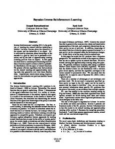
Fig. 1.

Control for inverted pendulum

(21)

J(θ) can be maximized by repeating the above E- and Msteps. Similarly, the on-line EM algorithm for the stochastic ¯ actor is derived. h(i|x c (t), u(t), θ(t − 1)) is calculated in the modified E-step. The step-wise equation (8a) is then replaced by hhf (xc , u)iii (t) =(1 − η(t))hhf (xc , u)iii (t − 1) + η(t) ¯ × f (xc (t), u(t))h(i|x c (t), u(t), θ(t − 1)). (22) In the modified M-step, the weighted means are updated by (22) and the new model parameter is determined by (8). D. Actor-critic learning The learning process for the actor-critic architecture process is as follows. 1) Control and critic-learning phase 1-1. For the current state xc (t), the current actor outputs a stochastic action u(t). The stochastic action is generated by using the stochastic NGnet in the following way. A unit i is selected with the conditional probability P (i|xc ) for state xc . After that, an action u(t) is generated with the conditional probability P (u|xc , i) for state xc and the selected i. 1-2. Using u(t), the system changes its state to xc (t+1) according to the system dynamics. The learning system observes reward r(xc (t), u(t)). 1-3. The on-line EM algorithm is used to train the critic. The input to the critic NGnet is the stateaction pair, i.e., (xc (t), u(t)). The target output is the right-hand side of (13). Note that the second right-hand side term can be defined for either the stochastic policy or the deterministic policy. We use the deterministic policy, which is defined by the expected output of the stochastic actor, because we use the deterministic actor after the training. Therefore, the target output for the critic NGnet is calculated using the current critic and the current deterministic actor, both evaluated at t + 1. The learning system repeats this process for a certain period of time (tmax ), using a fixed actor. In this period, the critic NGnet is modified to approximate

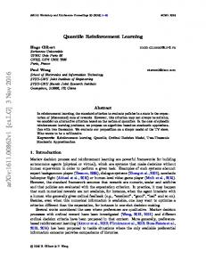
the Q-function for the fixed actor, and the state-action trajectory X ≡ { (xc (t), u(t)) | t = 1, 2, ..., tmax } is saved. 2) Actor-learning phase The actor NGnet is trained from the saved trajectory X by using the modified on-line EM algorithm described in Section 3.3. IV. E XPERIMENT In order to examine the performance of the above learning method, we consider two control tasks. The first task is to swing up and stabilize a single pendulum with a limited torque controller [4], [3]. The state of the system is denoted by xc ≡ (q, q), ˙ where q is the angle of the pendulum from the upright position and q˙ is the angular velocity. The torque u is assumed to be limited to the range |u| ≤ umax , where umax is not large enough to bring the pendulum up without swinging. The following process is conducted during a single learning episode. After the pendulum is released from the vicinity of the upright position, the learning system observes the system state and yields a control signal according to the stochastic actor at every 0.01 second. A reward r (xc (t), u(t)) is given by r˜ (xc (t + 1)), which is defined by ¡ ¢ r˜(xc ) = exp −q 2 /ν1 − q˙2 /ν2 , (23) where ν1 and ν2 are constants. The reward r˜(xc ) ∈ [0, 1] encourages the pendulum to stay in a high position. This control process is conducted for 7 seconds. The learning process for a single episode has been described in Section 3.4. The reinforcement learning proceeds by repeating these episodes. After 17 learning episodes, the system is able to stabilize the pendulum at the upright position from almost all initial states. For example, the system is able to swing-up and stabilize the pendulum at the upright position when the system initially stays still at the bottom. Figure 1 shows a stroboscopic timeseries of this control process. The second task is to balance an acrobot near an upright position [7]. The acrobot is the two-link underactuated robot depicted in figure 2. The second joint exerts torque while the first joint does not. This task is very difficult because the system has a nonlinear and unstable dynamics. After 18

after 40 (37) episodes. The new learning method is thus more efficient than the previous method.

M2 g u

L2

V. C ONCLUSION

q2

q1

In this article, we have proposed a new RL method, which has an architecture like the actor-critic model. The critic approximated the Q-function. The actor approximated a stochastic soft-max policy defined by the Q-function. The online EM algorithm is used to train the critic and the actor. The new method was applied to two automatic control problems and fairly good control was obtained after a few learning trials. We can thus confirm that our new RL method is based on a good function approximator and a fast learning algorithm, which are crucial for tasks that have continuous state and action spaces.

M1 g L1

Fig. 2.

The acrobot

Time Sequence of Balancing Acrobot

Height

2 1 0 0

0.5

1 Time (sec.)

1.5

2

R EFERENCES

Height

2 1 0 2

2.5

4

4.5

3 Time (sec.)

3.5

4

5

5.5

6

Height

2 1 0

Time (sec.)

Fig. 3.

Control for balancing acrobot

learning episodes, however, our method is able to make the acrobot stand straight up when the initial state is close to the upright position. Figures 3 and 4 show a typical control process after the learning. Figure 3 shows a stroboscopic time-series of the acrobot state and figure 4 shows the time sequence of the state and the control signal. The dashed (dotted) line denotes the angle of the first (second) joint and the solid line denotes the control signal. The system gradually suppresses the oscillation of the two joints and finally makes them stand straight up at the upright position. These two tasks were also examined in our previous studies [4], [7], where the actor’s deterministic NGnet was trained according to the on-line EM algorithm by using the gradient of the critic NGnet. In the previous method, good control for the inverted pendulum (for the balancing acrobot) was acquired Control Sequence of Balancing Acrobot 0.6

0.4

State ; Torque

0.2

0

−0.2

−0.4

−0.6

−0.8

q1/π q2/π u/20 0

1

2

Fig. 4.

3

4

5 Time (sec.)

6

7

8

State-control sequence

9

10

[1] Barto, A. G., Sutton, R. S. and Anderson, C. W.: Neuronlike adaptive elements that can solve difficult learning control problems, IEEE Transactions on Systems, Man, and Cybernetics, Vol. SMC-13, No. 5, pp. 834– 846 (1983). [2] Dempster, A. P., Laird, N. M. and Rubin, D. B.: Maximum likelihood from incomplete data via the EM algorithm, Journal of Royal Statistical Society B, Vol. 39, No. 1, pp. 1–38 (1977). [3] Doya, K.: Reinforcement learning in continuous time and space, Neural Computation, Vol. 12, No. 1, pp. 219–245 (2000). [4] Sato, M. and Ishii, S.: Reinforcement Learning based on On-line EM Algorithm, Advances in Neural Information Processing Systems 11, MIT Press, pp. 1052–1058 (1999). [5] Sato, M. and Ishii, S.: On-line EM algorithm for the normalized Gaussian network, Neural Computation, Vol. 12, No. 2, pp. 407–432 (2000). [6] Xu, L., Jordan, M. I. and Hinton, G. E.: An alternative model for mixtures of experts, Advances in Neural Information Processing Systems 7 (Tesauro, G., Touretzky, D. S. and Leen, T. K.(eds.)), MIT Press, pp. 633–640 (1995). [7] Yoshimoto, J., Ishii, S. and Sato, M.: Application of reinforcement learning to balancing of acrobot, 1999 IEEE International Conference on Systems, Man and Cybernetics, Vol. V, pp. 516–521 (1999).