context of engine idle-speed control; the algorithm is "rst applied in simulation on a nominal engine model, and this is
Control Engineering Practice 8 (2000) 147}154
On-line PID tuning for engine idle-speed control using continuous action reinforcement learning automata M. N. Howell, M. C. Best* Department of Aeronautical and Automotive Engineering, Loughborough University, Loughborough, Leicestershire, UK Received 3 February 1999; accepted 27 July 1999
Abstract PID systems are widely used to apply control without the need to obtain a dynamic model. However, the performance of controllers designed using standard on-line tuning methods, such as Ziegler}Nichols, can often be signi"cantly improved. In this paper the tuning process is automated through the use of continuous action reinforcement learning automata (CARLA). These are used to simultaneously tune the parameters of a three term controller on-line to minimise a performance objective. Here the method is demonstrated in the context of engine idle-speed control; the algorithm is "rst applied in simulation on a nominal engine model, and this is followed by a practical study using a Ford Zetec engine in a test cell. The CARLA provides marked performance bene"ts over a comparable Ziegler}Nichols tuned controller in this application. ( 2000 Elsevier Science Ltd. All rights reserved. Keywords: Learning automata; Intelligent control; PID (three term) control; Engine idle-speed control
1. Introduction Despite huge advances in the "eld of control systems engineering, PID still remains the most common control algorithm in industrial use today. It is widely used because of its versatility, high reliability and ease of operation (see for example Astron & Hagglund, 1995). A standard form of the controller is given in Eq. (1) and the implementation is shown in Fig. 1: u(t)"K e(t)#K p i
P
t
de(t) e(q) dq#K . d dt
(1) 0 The measurable output y(t) is subject to sensor noise n(t) and the system to disturbances d(t), both of which can be assumed unknown. The control u(t) is a summation of three dynamic functions of the error e(t) from a speci"ed reference (demand) output y (t). Proportional control 3%& has the e!ect of increasing the loop gain to make the system less sensitive to load disturbances, the integral of error is used principally to eliminate steady-state errors, and the derivative action helps to improve closed loop
* Corresponding author. Tel.: #44-1509-223-406; fax: #44-1509223-946. E-mail addresses:
[email protected] (M. N. Howell),
[email protected] (M. C. Best)
stability. The parameters K , K , K are thus chosen to p i d meet prescribed performance criteria, classically speci"ed in terms of rise and settling times, overshoot and steadystate error, following a step change in the demand signal. A standard method of setting the parameters is through the use of Ziegler}Nichols' tuning rules (Ziegler & Nichols, 1942). These techniques were developed empirically through the simulation of a large number of process systems to provide a simple rule. The methods operate particularly well for simple systems and those which exhibit a clearly dominant pole-pair, but for more complex systems the PID gains may be strongly coupled in a less predictable way. For these systems, adequate performance is often only achieved through manual and heuristic parameter variation. This paper introduces a formal approach to setting controller parameters, where the terms are adapted online to optimise a measure of system performance. The performance measure is usually a simple cost function of error over time, but it can be de"ned in any way, for example to re#ect the classical control criteria listed earlier. The adaptation is conducted by a learning algorithm, using Continuous Action Reinforcement Learning Automata (CARLA) which was "rst introduced by Howell, Frost, Gordon and Wu (1997). The control parameters are initially set using a standard Ziegler}Nichols method; three separate learning automata are then
0967-0661/00/$ - see front matter ( 2000 Elsevier Science Ltd. All rights reserved. PII: S 0 9 6 7 - 0 6 6 1 ( 9 9 ) 0 0 1 4 1 - 0
148
M. N. Howell, M. C. Best / Control Engineering Practice 8 (2000) 147}154
Fig. 1. PID controller implementation.
employed * one for each controller gain * to adaptively search the parameter space to minimise the speci"ed cost criterion. As an example, a PID controller is developed for load disturbance rejection during engine idle. The idle-speed control problem presents particular challenges, due to system nonlinearities, and varied predictable and unpredictable noise conditions, and the application has attracted much research interest over many years. A thorough review of the state of the art was given in Hrovat and Sun (1997), and recent works on control algorithms have included SISO robust control (Glass & Franchek, 1999) and a combination of L1 feedforward and LQG feedback control (Butts, Sivashankar & Sun, 1999). In this paper, the PID algorithm is "rst tuned in simulation, to an essentially linear engine idle model; it is then re-examined on a physical engine in a test cell. In both cases the throttle angle is used to regulate measured engine speed.
2. Continuous action reinforcement learning automata The CARLA operates through interaction with a random or unknown environment by selecting actions in a stochastic trial and error process. For applications that involve continuous parameters which can safely be varied in an on-line environment, the CARLA technique can be considered to be more appropriate than alternatives. For example, one such alternative, the genetic algorithm (Holland, 1975) is a population-based approach and thus requires separate evaluation of each member in the population at each iteration. Also, although other methods such as simulated annealing could be used, the CARLA has the advantage that it provides additional convergence information through probabilitiy density functions. CARLA was developed as an extension of the discrete stochastic learning automata methodology (see Narendra and Thathachar (1989) or Najim and Posnyak (1994) for more details). CARLA replaces the discrete action space with a continuous one, making use of continuous probability distributions and hence making it more appropriate for engineering applications that are inherently continuous in nature. The method has been successfully applied to active suspension control
Fig. 2. Learning system.
(Howell et al., 1997) and digital "lter design (Howell & Gordon, 1998). A typical layout is shown in Fig. 2. Each CARLA operates on a separate action * typically a parameter value in a model or controller * and the automata set runs in a parallel implementation as shown, to determine multiple parameter values. The only interconnection between CARLAs is through the environment and via a shared performance evaluation function. Within each automata, each action has an associated probability density function f (x) that is used as the basis for its selection. Action sets that produce an improvement in system performance invoke a high-performance &score' b, and thus through the learning sub-system have their probability of re-selection increased. This is achieved by modifying f (x) through the use of a Gaussian neighbourhood function centred on the successful action. The neighbourhood function increases the probability of the original action, and also the probability of actions &close' to that selected; the assumption is that the performance surface over a range in each action is continuous and slowly varying. As the system learns, the probability distribution generally converges to a single Gaussian distribution around the desired parameter value. Referring to the ith action (parameter), x is de"ned on i a pre-speci"ed range Mx (min), x (max)N. For each iteri i ation k of the algorithm, the action x (k) is chosen using i the probability distribution function f (x , k), which is i i initially uniform: f (x ,1)" i i 1/[x (max)!x (min)] where x 3Mx (min), x (max)N, i i i i i 0 otherwise. (2)
G
The action is selected by
P
xi (k) f (x , k) dx "z (k), i i i i 0 where z varies uniformly in the range M0, 1N.
(3)
M. N. Howell, M. C. Best / Control Engineering Practice 8 (2000) 147}154
With all n actions selected, the set is evaluated in the environment for a suitable time, and a scalar cost value J(k) calculated according to some prede"ned cost function. Performance evaluation is then carried out using
G G
HH
J !J(k) b(k)"min max 0, .%$ ,1 , (4) J !J .%$ .*/ where the cost J(k) is compared with a memory set of R previous values from which minimum and median costs J , J are extracted. The algorithm uses a re.*/ .%$ ward/inaction rule, with action sets generating a cost below the current median level having no e!ect (b"0), and with the maximum reinforcement (reward) also capped, at b"1. After performance evaluation, each probability density function is updated according to the rule f (x , k#1)" i i a(k)[ f (x , k)#b(k)H(x , r)] if x 3Mx (min), x (max)N, i i i i i i 0 otherwise, (5)
G
where H(x, r) is a symmetric Gaussian neighbourhood function centred on the action choice, r"x(k):
A
H(x, r)"
B A
g (x!r)2 h exp ! 2(g (x !x ))2 (x !x ) w .!9 .*/ .!9 .*/
B (6)
and g and g are free parameters that determine the h w speed and resolution of the learning by adjusting the normalised &height' and &width' of H. These are set to g "0.02 and g "0.3 along with a memory set size for w h b(k) of R"500, as a result of previous investigations which show robust CARLA performance over a range of applications (Howell et al., 1997, 1998; Frost, 1998).
149
The parameter a(k) is chosen in Eq. (5) to renormalise the distribution at k#1, 1 a" . (7) :xii (.!9)[ f (x , k)#b(k)H(x , r)] dx x (.*/) i i i i For implementation, the distribution is stored at discrete points with equal inter-sample probability, and linear interpolation is used to determine values at intermediate positions. A summary of the required discretisation method is given in the appendix, or for more details see Frost (1998).
3. Engine idle-speed control Vehicle spark ignition engines spend a large percentage of their time operating in the idle-speed region. In this condition the engine management system aims to maintain a constant idle speed in the presence of varying load demands from electrical and mechanical devices, such as lights, air conditioning compressors, power steering pumps and electric windows. Engines are inherently nonlinear, incorporating variable time delays and discontinuities which make modelling di$cult, and for this reason their control is well suited to optimisation using learning algorithms. 3.1. Model-based learning For comparison with real engine data, and as a demonstration of CARLA operation, the technique is "rst tested on a simple generic engine model. Cook and Powell (1988) presented a suitable structure, which relates change in engine speed to changes in fuel spark and throttle, with the model linearised about a "xed idle speed. Fig. 3 illustrates the model, with attached PID controller.
Fig. 3. Engine idle-speed simulation model.
150
M. N. Howell, M. C. Best / Control Engineering Practice 8 (2000) 147}154
Component dynamics are taken as 20 K ¹ p p , Gr(s)" , Ga(s)"G e~sq, Gi(s)" p (3.5s#1) (¹ s#1) p (8) where nominal system parameters are chosen: ¹ "0.05, p K ¹ "9000, G "0.85, K "1]10~4 with a combusp p p n tion time delay of q"0.1 s. From earlier identi"cation work, these settings are known to be representative of the test engine which we will consider in Section 3.2, for an idle speed of 800 rpm with no electrical or mechanical load. In this paper, control is applied via modulation of the throttle only, to minimise the change in engine speed (*