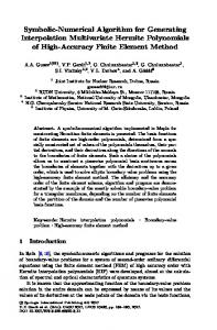
2Department of Mechanical Engineering, The Ohio State University, 650 Ackerman Rd, ... Columbus, OH 43202, USA ...... Thus our job is to perform on-line sym- .... center Bo and the contact forces acting at the point of contact with A, may be.
Multibody System Dynamics (2005) 14: 387–417
C �
Springer 2005
On-Line Symbolic Constraint Embedding for Simulation of Hybrid Dynamical Systems R. BRENT GILLESPIE1 , VOLKAN PATOGLU1 , ISLAM I. HUSSEIN1 and E.R. WESTERVELT2 1 Department
of Mechanical Engineering, University of Michigan, 2350 Hayward Ave, Ann Arbor, MI 48109, USA 2 Department of Mechanical Engineering, The Ohio State University, 650 Ackerman Rd, Suite 255, Columbus, OH 43202, USA (Received: 28 June 2004; accepted in revised form: 27 June 2005) Abstract. In this paper we present a simulator designed to handle multibody systems with changing constraints, wherein the equations of motion for each of its constraint configurations are formulated in minimal ODE form with constraints embedded before they are passed to an ODE solver. The constraint-embedded equations are formulated symbolically according to a re-combination of terms of the unconstrained equations, and this symbolic process is undertaken on-line by the simulator. Constraint-embedding undertaken on-the-fly enables the simulation of systems with an ODE solver for which constraints are not known prior to simulation start or for which the enumeration of all constraint conditions would be unwieldy because of their complexity or number. Issues of drift associated with DAE solvers that usually require stabilization are sidestepped with the constraintembedding approach. We apply nomenclature developed for hybrid dynamical systems to describe the system with changing constraints and to distinguish the roles of the forward dynamics solver, a collision detector, and an impact resolver. We have prototyped the simulator in MATLAB and demonstrate the design using three representative examples. Keywords: symbolic manipulation, changing constraints, constraint embedding, hybrid dynamical systems
1. Introduction Various methods are available for the production of the equations of motion for constrained multibody systems, and each method typically produces the equations in a particular form. While the equations are equivalent in the sense that they possess the same solution, the form of the equations usually dictates which of several available numerical methods may be applied to obtain a solution. While the following classification is not exhaustive, let us identify three major families for the production and solution of constrained multibody systems [1]: (1) constraint appending using the method of Lagrange multipliers, which produces differential algebraic equations (DAEs) for solution by a DAE solver, (2) projecting the unconstrained equations through a matrix produced numerically, which produces DAEs or ODEs requiring stabilization, and (3) symbolic constraint embedding, which produces ODEs.
388
R. B. GILLESPIE ET AL.
Basically, a whole spectrum of techniques is available to account for the effects of constraints: from the symbolic constraint embedding methods applied during formulation to numerical multiplier and projection methods applied during simulation by a DAE solver. The constraint-embedding approach is appealing because it permits one to apply an ODE solver, which generally requires less expertise than a DAE solver. Since the constraint-embedded equations contain only those variables that are associated with the degrees of freedom of the constrained system, the solution cannot stray from the constraint manifold and does not require stabilization. Also, the constraint-embedded equations are fewer in number and have fewer unknowns than their constraint-appended counterparts, which can lead to compact and numerically efficient equations, though such an outcome also requires the judicious use of generalized speeds (quasi-velocities) [2, 3].1 On the other hand, DAE solvers offer a solution to the constrained system dynamics without requiring the symbolic operations involved in eliminating dependent variables. One simply needs to invoke a high index DAE solver or negotiate the options available for index reduction and stabilization to ensure that the DAE solver provides a solution that satisfies the requirements of a given application [4]. Now, in certain multibody systems, changes in constraint conditions are likely to occur during the time period in which the solution of the equations of motion is desired. Such systems are said to have changing topology [5, 6] or intermittent motion [7]. Choosing a solution method and concomitantly choosing a formulation method requires special consideration for such systems. At first glance, it appears that only the numerical approach embodied in DAE solvers can be readily adapted for treatment of changing constraints. The core unconstrained equations remain untouched through the change in constraint using the constraint-appending or numerical projection methods. Thus, changes in constraint may be reflected simply by changing the constraint equations that are imposed numerically during each epoch of the simulation [7]. Use of constraint-embedding, on the other hand, would require re-formulation of the entire set of equations upon each change in constraint condition. If all constraint conditions can be enumerated prior to simulation, then quite plausibly the various constrained system formulations could be linked together at run-time to form a hybrid dynamical system [8]. However, the ability to handle constraints that are not specified prior to the start of simulation would require the incorporation of symbolic manipulation routines into the run-time solution code. This might seem like an unlikely approach, given the computational demands and very distinct heritage of symbolic methods and numerical methods. However, that is precisely what we have undertaken in our work and demonstrate in this paper. Another motivating issue for the development of on-line constraint embedding lies in the treatment of representation singularities. For certain mechanisms (e.g., 1The
reduced equations are often dismissed as less numerically efficient [1, 4], especially given the availability of sparse matrix techniques for the constraint-appended equations. However, the use of generalized speeds is not usually considered in such estimations.
ON-LINE SYMBOLIC CONSTRAINT EMBEDDING FOR HYBRID DYNAMICAL SYSTEMS
389
robots, spacecraft) it may prove difficult to define a single set of independent motion variables suitable for all regions of the coordinate space. In such cases, a change in the choice of independent motion variables may be undertaken during simulation to avoid break-down of the solution method. Again, although the DAE approach essentially avoids this problem since it does not rely on a model in independent coordinates, the development of on-line constraint embedding, by incorporating symbolic routines into the run-time simulator code, would allow ODE solvers to be applied. Detection of the suitability of the active set of independent coordinates can be accomplished using a check of the condition number of the constraint Jacobian, and a new set can be chosen and re-formulation undertaken to avoid simulator crash, as described in [9]. We propose to apply computerized symbolic algebra not only to the process of formulating equations of motion, but also to the process of simulation. Our aim is to expand the tools available for simulation of systems with changing topology to the point where they will reflect the variety of options available for constant topology systems. We anticipate applications in which the relative simplicity and stability of ODE solvers are desired and the ability to impose the effects of constraints whose specifications are not available prior to run-time is required. We also anticipate the availability of sufficient computational power to invoke the symbolic operations necessary for eliminating dependent coordinates within a single time-step in a constant step-size solver. This would enable hardware- or humanin-the-loop simulation for systems with changing constraints, where the particular constraint conditions in effect are driven by a human or piece of hardware linked to the simulated dynamics through a computer interface. Examples of systems in which unforseen constraints may be imposed during run-time include shared gaming environments, where objects passed between users or agents are subject to on-line modifications of their surface shape. Another example is a design environment in which multiple users can collaborate on the specification of a virtual artifact. Changes to the shape of an object, especially re-parameterizations of shape will require on-line symbolic re-formulation of the constrained equations in independent coordinates if an ODE solver is to be used. On-line formulation allows data-hiding in a distributed simulation environment. That is, the parameterization of the shape of an object may be hidden from the simulation routine until the constraint is actually imposed. For example, the dynamics of two contacting bodies, each described in separate but networked computational environments, might be described in an independent coordinate formulation that draws the surface shape descriptions from the networked computers only upon contact. The simulation then becomes reactive, able to support interaction, even through teleoperation, with other human or software agents. A second class of applications that motivates on-line constraint embedding lies in systems for which the enumeration of all constraint conditions prior to simulation would be unwieldy because of their complexity or number. On-line constraint embedding allows only those constraints to be considered that are actually encountered during simulation.
390
R. B. GILLESPIE ET AL.
We are particularly interested in the use of on-line constraint embedding to create virtual environments for exploration by a human user through a haptic interface. Our simulator is intended to facilitate interaction with mechanisms that include escapements, stops, and latches specified by a geometric model that retains significant independence from the dynamic solution engine. Our simulator treats collisions and transitions between free, rolling, and sliding motion, all with an ODE solver. We aim to reproduce the effects of making, possibly maintaining, and breaking contact between bodies, knowing that these effects are often incited by a user exploring a virtual environment. Naturally, interaction with a user in a virtual environment requires real-time simulation. We have prototyped a simulator with on-line constraint embedding in MATLAB. Development of the equations of motion is based on Kane’s method and the on-line re-formulation in independent coordinates is based on a re-combination of terms in the unconstrained equations according to the algorithm outlined in [10] and further extended in [3]. Although our simulator is currently not capable of realtime constraint embedding within a single time-step in a fixed-step solver, we do demonstrate embedding on-the-fly that runs in parallel with simulation and that is initiated a short period before the new constrained equations are needed. In the following sections, we further review the field of constrained system formulation and simulation, contrasting on-line constraint embedding to existing methods. Thereafter, we develop nomenclature from the field of hybrid dynamical systems that we use to lay out our simulator design. Finally, we demonstrate the simulator in three examples and conclude.
2. Dynamical System Modelling 2.1.
KINEMATICAL AND DYNAMICAL DIFFERENTIAL EQUATIONS
Consider a multibody system S whose configuration is described by n generalized coordinates qr (r = 1, . . . , n). To enable the formulation of compact and efficient equations of motion [11], one may define n generalized speeds u r (r = 1, . . . , n) as linear combinations of the generalized coordinate derivatives q˙ r (r = 1, . . . , n) [2]. One may express these definitions using �
u = Y q˙ + Z ,
(1)
where u and q˙ are n × 1 matrices of u r and q˙ r , and where the elements of the n × n matrix Y and n × 1 matrix Z are functions of qr (r = 1, . . . , n) and possibly time t. The matrices Y and Z in Equation (1) must be chosen by the analyst in such a way that the reciprocal relations exist in which the generalized coordinate derivatives are expressed in terms of the generalized speeds: q˙ = W u + X,
(2)
ON-LINE SYMBOLIC CONSTRAINT EMBEDDING FOR HYBRID DYNAMICAL SYSTEMS
391
where the elements of the n × n matrix W and n × 1 matrix X are functions of qr (r = 1, . . . , n) and possibly time t. Equation (2) is a matrix arrangement of the kinematical differential equations, and forms the first of two portions of the state equations or equations of motion that govern the behavior of system S. The second portion, the dynamical differential equations, may be expressed in matrix form as M(q)u˙ = f(q, u, t)
(3)
which may be derived, for example, using Kane’s method. In Kane’s method, one carries out dot products between partial velocity vectors and applied and inertia forces, and between partial angular velocity vectors and applied and inertia torques. The partial velocity and partial angular velocity vectors are obtained by inspection of the pertinent velocity and angular velocity expressions, identifying coefficients of the corresponding generalized speeds. Then, a summation of terms over all particles and bodies in S produces expressions for the generalized active force Fr (r = 1, . . . , n) and the generalized inertia force Fr∗ (r = 1, . . . , n). The dynamical differential equations are then contained in Fr + Fr∗ = 0 (r = 1, . . . , n), which may be arranged as in Equation (3). If for all configurations of the system the motions of all bodies are resisted by inertia, then the mass matrix M is nonsingular and the equations of motion can also be expressed in explicit form as u˙ = F(q, u, t)
(4)
where F is a n × 1 matrix of generalized applied and inertia force terms. In this paper, we will focus on systems for which the mass matrix is nonsingular, since this is the case for the majority of systems of engineering interest. We refer readers to Chapter 6 in [12] for a detailed treatment of the singular case. 2.2.
CONSTRAINT EQUATIONS
System S may be subject to constraints, including constraints that act only during a time segment within the time interval of interest. Suppose there are l configuration constraints given as Φ(q) = 0.
(5)
In certain formulations, to be reviewed in the next section, configuration constraints are treated as motion constraints by differentiating them with respect to time: Φq q˙ = 0.
(6)
392
R. B. GILLESPIE ET AL.
The configuration q can be found by integrating the kinematical differential equations (2). However, round-off or initialization errors in the motion constraints may lead to violations of the configuration constraints in Equation (5). More significantly, in the case of configuration constraints that are differentiated to form Equation (6) and then embedded in the dynamical differential equations, drift introduced by integration will also lead to violations of the configuration constraints. These violations can accumulate and slow down the integration over long simulations. Since the errors at the motion (velocity) level will remain relatively constant during integration [1], the violation to the configuration constraints will only grow linearly with time. To mitigate these drift errors, the configuration constraints may be imposed within the solver by, say, performing Newton iterations on Equation (5) at each time step (see, for example, Section IV in [13]). Alternatively, stabilization techniques may be used to overcome the problem of drift [11]. Let there be an additional m − l motion constraints, where l ≤ m ≤ n. Suppose further that the motion constraints are linear in the u r , so that after the application of Equation (2), the differentiated configuration constraints can be combined with the motion constraints, yielding Bu + C = 0,
(7)
where the elements of the m × n matrix B and the m × 1 matrix C are functions of qr (r = 1, . . . , n) and possibly time t. Some of the index reduction formulations require that the constraints (7) be differentiated to the acceleration level ˙ + C˙ = 0, B u˙ + Bu
(8)
so that they can be solved together with the dynamical differential equations. Care should be taken when imposing acceleration level constraints instead of their motion-level or configuration level counterparts since in this case the drift phenomenon is critical. The initialization and numerical errors that occur at the acceleration level will lead to motion-level violations that grow linearly and configurationlevel violations that grow quadratically in time. Therefore, it is always good practice to use stabilization with these formulations. Equations (4) together with configuration and motion constraints form a system of n first-order differential and m algebraic equations to be solved for the n generalized speeds u r . Note that the n first-order kinematical differential Equations (2) are typically solved alongside Equations (4) and (7) to determine the generalized coordinates qr . Although we have identified more equations than unknowns, the system is in fact not overdetermined, since associated with the constraint equations are constraint forces that restrict the motion of S. There will be m constraint force components,
ON-LINE SYMBOLIC CONSTRAINT EMBEDDING FOR HYBRID DYNAMICAL SYSTEMS
393
Figure 1. Four designs for a simulator based on (I) The Method of Lagrange Multipliers, (II) Projection Matrices, (III) Off-line Constraint Embedding, and (IV) On-line Constraint Embedding (introduced in this paper). Parameter n stands for the number of generalized speeds, � m stands for the number of algebraic constraints and p = n − m. Stacked and shaded boxes indicate the manner in which each approach may be adapted to treat systems with changing constraints.
one for each degree of freedom that is restricted. Let us call the constraint force components ξs (s = 1, . . . , m). There are three general approaches to the analysis of constrained dynamical systems as discussed in Section 1. The first employs the method of Lagrange multipliers, the second a numerical projection matrix R, and the third is constraint embedding. The next section discusses these formulations along with their implementation in simulators to handle systems with changing constraints.
3. Approaches to the Formulation and Simulation of Systems Subject to Changing Constraints Figure 1 shows schematically four possible designs for an interactive simulator capable of handling systems subject to changing constraints.2 This section will be organized around Figure 1. The information contained in each schematic representation is twofold. First, the labelled boxes indicate the number of dynamical differential equations and algebraic constraint equations and make the distinction 2 There
exist other alternatives that will not be considered in this paper. One of them is based on computing the constraint forces explicitly as the solution of a linear complementarity problem and applying them to the unconstrained system of equations [14, 15]. Satisfaction of the constraints then follows by the action of the constraint forces, through the dynamical analysis.
394
R. B. GILLESPIE ET AL.
between the use of the constraints to eliminate dependent coordinates and their use to augment the analysis. Secondly, the arrangement of shaded boxes depicts how each simulator is cast to handle changing constraints. Design I is based on the method of Lagrange multipliers. After the unconstrained system of equations is developed, the method of Lagrange multipliers is used to append the constraint equations, by introducing m multipliers λs (s = 1, . . . , m) and adding the term B T λ to Equation (3) leading to M(q)u˙ = f(q, u, t) + B(q)T λ
(9)
where λ is a m × 1 column matrix of undetermined multipliers. The multipliers λ are linear combinations of the constraint force components [16]. If no motion constraints are imposed, Equation (9) may be solved together with Equation (5) as a DAE of index-3. Although index-3 solvers are available [17], the algebraic constraint equations are usually differentiated once or twice to reduce their index and thus prepare the equations for the more readily available index-2 or index-1 DAE solvers. Solving Equation (9) together with Equation (7) produces a DAE of index-2 or solving with Equation (8) produces an index-1 DAE. Both index-1 and index-2 formulations require stabilization to the constraint manifold since information is lost when differentiating the constraint equations. Baumgarte stabilization [18] and the Augmented Lagrangian formulation [19] are among the numerous stabilization methods available for index-1 formulations. A stabilized formulation also exists for index-2 DAEs [20]. For the treatment of systems with changing constraints using the simulator architecture of Design I, the core n equations, Equation (9), remain the same throughout the simulation (except for the constraint Jacobian B(q), which reflects only the active constraints). The m active algebraic constraint equations are applied to the integration and may change during simulation. The simulator designs described in [7, 21] fit Design I. In [7, 22], Haug et al. demonstrated the management of constraints within the method of Lagrange multipliers and the use of DAE solvers. Design II makes use of numerical projection methods. The n unconstrained � equations, Equation (9), are projected onto the p = n − m dimensional constraint manifold by pre-multiplying with a p × n projection matrix R, which is produced numerically during solution from the constraint Jacobian B via SVD [23], QR decomposition [24], or Gauss triangularization [25]. The projection matrix R satisfies the equation R T B T = 0, and the projected dynamical differential equations are given by R T M u˙ = R T f.
(10)
These numerically projected equations require simultaneous solution of the constraint equations, so that together with the constraint equations, the problem may be formulated as an index-2 DAE of p + m = n equations. Twice differentiating
ON-LINE SYMBOLIC CONSTRAINT EMBEDDING FOR HYBRID DYNAMICAL SYSTEMS
395
the configuration constraints produces an ODE, although its solution again requires stabilization. For the treatment of systems with changing constraints, the simulator architecture of Design II features p dynamical equations produced by numerical projection. The m algebraic constraint equations are solved simultaneously, and the dynamical equations must be projected using a new projection matrix each time the constraints change. Adaptation of the projection method to handle changing constraints is relatively easy since whenever a change in constraints occurs, only the projection matrix R is affected due to the change in constraint Jacobian B; however, R is already generated on the fly numerically. In Design III and Design IV, the configuration constraints are differentiated and grouped with the motion (nonholonomic) constraints to produce constraint equations that are linear in the motion coordinates, as in Equation (7). These constraints are then used to undertake a local coordinate transformation to eliminate dependent motion variables from the equations [2]. This process projects the dynamical differential equations onto the p-dimensional constraint manifold, in which the solution of Equation (4) is constrained to lie. Here the projection is carried out using symbolic operations (realizing a dot product) in contrast to numerical operations and is called embedding the constraints. For a geometrical interpretation of the projection operation carried out in Kane’s method, see [26, 27]. To embed the constraints in Kane’s method, one expresses the m dependent generalized speeds in terms of the remaining p independent generalized speeds by carrying out linear operations on the constraint Equation (7). One may begin by re-ordering and partitioning the generalized speeds in Equation (7) to produce u p+1 u1 .. .. B1 . = B2 . + C. (11) un up where u r (r = 1, . . . , p) are the independent generalized speeds and u r (r = p + 1, . . . , n) are the dependent generalized speeds. Further, one must choose the B1 and B2 matrices so that Equation (11) may be solved uniquely for the dependent generalized speeds and the results written in terms of D = B1−1 B2 and E = B1−1 C as: u p+1 u1 .. .. (12) . = D . + E, un up where the elements of D and E are functions of qi (i = 1, . . . , n) and possibly time t. Now that the motion constraints have been expressed in an explicit linear form, the derivation of the constrained dynamical differential equations may proceed
396
R. B. GILLESPIE ET AL.
according to one of two methods. In the first, Equation (12) may be used to eliminate the dependent generalized speeds from the analysis and Kane’s method applied as usual. Alternatively, the constrained dynamical equations can be obtained by a recombination of terms from the unconstrained dynamical equations. Specifically, the constrained generalized active force F˜ r (r = 1, . . . , p) and the constrained generalized inertia force F˜ r∗ (r = 1, . . . , p) may be formed from the unconstrained generalized active force Fr (r = 1, . . . , n) and unconstrained generalized inertia force Fr∗ (r = 1, . . . , n) as follows: F˜ r = Fr + F˜ r∗ = Fr∗ +
n � s= p+1 n �
Dsr Fs Dsr Fs∗
(r = 1, . . . , p) (r = 1, . . . , p)
(13) (14)
s= p+1
where D was defined in Equation (12). To eliminate the dependent generalized speeds and dependent generalized speed derivatives from the resulting expressions, one may substitute from the motion constraints (Equation (12)) and differentiated motion constraints [3, 10]. See also Equations (4.4.3) and (4.11.4) in [2]. The equations of motion in the independent generalized speeds are then simply formed as: F˜ r + F˜ r∗ = 0 (r = 1, . . . , p)
(15)
which are only p ordinary differential equations in the p unknowns, u r (r = 1, . . . , p). Finally, Equation (15) may be used to produce explicit equations for u˙ r in the form ˜ u˙˜ = F(q, u, ˜ t)
(16)
where u˜ is a p × 1 matrix of the independent generalized speeds. The resulting dynamic differential equations are a set of ordinary differential equations, and yield to solution under a standard ODE solver. Advantages associated with embedding constraints include the reduction in the number of equations to be integrated and robustness due to the disappearance of the instability problem associated with the integration of differentiated constraints in DAE solvers. For treating systems subject to changing constraints, simulator Design III features switching among a set of ODEs, each produced by embedding the pertinent constraints. Since the constraints are embedded, there are only p dynamical equations to solve for the system in each of its constraint conditions where p may vary by condition. However, in Design III, all of the constraints must be known prior to the time of simulation. Such an approach is often suitable for the simulation of mechanisms, as described in [8].
ON-LINE SYMBOLIC CONSTRAINT EMBEDDING FOR HYBRID DYNAMICAL SYSTEMS
397
The simulator architecture depicted in Design IV is the scheme proposed in this paper. As in Design III, the constraints are embedded, yielding only p dynamical differential equations for the system in each of its constraint conditions. However, unlike Design III, the constraints are embedded on-line (during simulation) through symbolic manipulation of the dynamical equations. Thus, the equations resident in the integrator are not simply swapped in and out; they are subject to reformulation on the fly. The incorporation of on-line formulation into the simulator design allows updates to the geometric model that occur during simulation to be reflected in the behavior of the dynamic model. The process outlined above for obtaining equations of motion is aided by the use of symbolic manipulation software. One such symbolic package is Autolev [28, 29] and another is SymSim, a toolbox for MATLAB created by the authors and described in Section 5.5 below. The recombination of terms prescribed in Equations (13) and (14) is carried out during simulation using computerized symbolic algebra to produce the equations in minimal form for the system in each of its constraint conditions, just before they are needed by the numerical solver. Before demonstrating the process, we first introduce some notation for hybrid dynamical systems, and then describe its incorporation with two additional simulator components: a collision detector and an impact resolution algorithm. In the following, we review the language of hybrid dynamical systems and apply it to the formulation of a simulator to handle the interacting continuous-time and discrete-time dynamics. The intention is to capture both the “memory” in the continuous system dynamics and the “memory” in the discrete dynamics and their interaction to create a system whose behavior accurately reflects the behavior of its target system.
4. Hybrid System Modelling To prepare for the construction of a simulator that can advance the solution of a constrained dynamical system through changes in the constraints, we borrow nomenclature and modeling tools from the field of hybrid dynamical systems. Review papers in the field of hybrid dynamical systems include [30, 31]. The purpose of this section is to present a model that can sequentially and interactively patch together various dynamical subsystems with appropriate initial and final states. Hybrid dynamical systems are systems that exhibit interacting discrete state and continuous state dynamics. The term interacting indicates that changes in discrete states influence the evolution of the continuous dynamics and changes in continuous states influence evolution in the discrete dynamics. Such interaction precludes an analysis that treats the continuous and discrete models separately. We shall concentrate here on hybrid dynamical systems in which the discrete and continuous dynamics interact only at discrete points in time known as events.
398
R. B. GILLESPIE ET AL.
This enables a description in terms of a single discrete state subsystem, a collection of continuous state subsystems, and a description of the possible interactions between the two subsystem classes. We will also restrict the discussion to systems in which the continuous state dynamics can be modelled in the form of ODEs or DAEs, defined on open subsets of the time interval of interest. That is, we employ a continuous time formulation, realizing that these continuous dynamics will be solved numerically. To describe the discrete subsystem, we employ a finite state machine. Together, the collection of continuous and discrete subsystems expressed in this form may be represented in a hybrid automaton [30, 32]. A hybrid automaton, then, can be considered a finite state machine in which the discrete states have been replaced by so-called “modes”, each of which indicates a particular continuous dynamics. Each mode is a description of a dynamical system that applies for a period of time whose extent is governed by the discrete dynamics. While the continuous state may change at each instant, the state of the discrete subsystem changes only at the events. At these events, the discrete subsystem exerts its influence over the continuous dynamics in one or both of two ways: (a) by causing a switch in the active differential equations describing the continuous state evolution, and/or (b) by causing a jump or discontinuity in the continuous states. �n m The hybrid dynamics are abstracted into a collection S = k=1 Sk , of modes Sk , where n m is the number of modes and where the state x (k) within each mode Sk evolves according to the differential equation
x˙ (k) = Γ(k) x(k) , θ (k) , t ,
(17)
where θ (k) (t) is an exogenous input for the k-th mode. The superscripts (k) index not only the functions Γ but also the state x and input θ to allow different state and input variable definitions and possibly different state and input dimensions between modes. Note that for the simulation of mechanical systems, whose state equations are generally second order, the state x will comprise the generalized coordinates qr (r = 1, . . . , n) and the generalized speeds u r (r = 1, . . . , p). Also associated with each mode Sk is a set of pending transitions Jk to other modes, where j ∈ J (k) is the index of the new mode following the event and J (k) is the set of modes reachable from the k-th mode. The timing of the events is determined by a switching condition:
(k) (k) f j,i x , θ (k) = 0,
i = 1, . . . , n (k) j ,
j ∈ J (k) ,
(18)
where n (k) j is the number of transitions from mode k to mode j. The time t ∗ that, together with the state x(k) (t ∗ ) and specified motion θ (k) (t ∗ ), (k) produces a zero of switching condition f j,i is called a switching instant; it triggers the associated transition. Once a transition is triggered, an associated reset map φ (k) j,i
ON-LINE SYMBOLIC CONSTRAINT EMBEDDING FOR HYBRID DYNAMICAL SYSTEMS
399
Figure 2. An example hybrid automaton with three modes and five transitions.
is executed to map the final state values x(k) in the current mode to the initial state values x( j) in the next mode (k) ∗
x( j) = φ (k) j,i x , t ,
i = 1, . . . , n (k) j ,
j ∈ J (k) .
(19)
A special reset map sets the initial conditions for the initial mode S1 (the initial mode is arbitrarily labelled with k = 1) x(1) (0) = x(1) 0 .
(20)
Evaluation of the hybrid system can be viewed as a sequence of subproblems, each characterized by a continuous evolution in a mode terminated by an event (i.e., zero crossing of a switching condition), and then evaluation of the reset maps to initialize the new mode. It is convenient to represent the interacting continuous and discrete dynamics of the hybrid system using an automaton as in Figure 2. This simple hybrid automaton has 3 modes with two transitions from mode 1 to 2, one transition from mode 2 to 3, one transition from mode 3 to 1 and a self transition in mode 3.
5. Simulator Architecture A simulator equipped to handle multibody systems with changing constraint conditions requires three major components: a forward dynamics solver (an ODE or DAE solver), a collision detector, and a means for resolving impacts as indicated in the flow chart in Figure 3. The forward dynamics solver advances the solution of Γ(k) in continuous time between events. The collision detector checks for contact between (k) bodies by evaluating a collection of switching conditions f j,i (Additional switching conditions are used to detect interaction forces that become tensile between unilaterally constrained bodies, to trigger loss of contact). The impact resolver, triggered into action by the collision detector, computes reset maps φ (k) j,i to initialize the forward dynamics solver.
400
R. B. GILLESPIE ET AL.
Figure 3. Standard simulation flow chart.
Alongside these three major simulator components, there exist three models for the system: a dynamic model, a geometric model, and a contact model. Roughly, the numerical integrator will maintain the dynamic model, the collision detector handles the geometric model, and the impact resolver calls upon the contact model. The impact resolver however, also consults the geometric model and possibly the dynamic model to compute the appropriate impulse response between bodies. The use of a collision detector and impact resolver as in Figure 3 ensures that interacting bodies respond to each other’s presence. Note that the impact resolver is called only intermittently whereas the collision detector and forward dynamics solver run continually, either alongside or subsequent to each other in computational time. Let us now consider each of the elements of the flow chart in greater detail. 5.1.
FORWARD DYNAMICS SOLVER
The forward dynamics solver operates on the equations of motion, a set of differential equations in the configuration and motion variables and inertia parameters.
ON-LINE SYMBOLIC CONSTRAINT EMBEDDING FOR HYBRID DYNAMICAL SYSTEMS
401
The multibody model can contain embedded or appended configuration or motion constraint equations written in terms of certain geometric parameters that are not necessarily part of the geometric model. In addition to new initial conditions from the impact resolver, the forward dynamics solver may respond to forces and moments applied during simulation, perhaps through the action of a human user interacting through a haptic interface. 5.2.
COLLISION DETECTOR
A collision detector is an algorithm that operates on a continually updated geometric model to determine points in time at which objects make contact with one another. At initial contact, the collision detector triggers the impact resolution algorithm that computes the interaction forces or impulses that act, in simulation, to prevent interpenetration of the two colliding objects. A set of surface patches and their interconnection can be used to describe the geometry of each body in the simulation environment. The whole collection of surface patches along with its connected graph is called the geometric model. There exists an extensive literature on the collision detection problem. For a detailed overview of existing methods for different geometric representations, we refer the reader to survey papers [33, 34]. In previous work [35], we have also contributed a collision detector that treats objects whose boundaries are represented using parametric surface patches. In [35] we presented a method for finding and tracking the closest points between two parametric surfaces based on a control problem formulation and the design of a stabilizing controller. The algorithm simultaneously accounts for the surface shape and motion while asymptotically achieving (and maintaining) the closest points. Features of this approach include its guaranteed stability and seamless integration with the forward dynamics solver. 5.3.
IMPACT RESOLVER
Impact resolution considers the problem of finding the separation velocities of two contacting bodies given the approach velocities and an appropriate contact model. Using Kane’s method, the problem is formulated by expressing generalized impulse and momentum in terms of independent generalized speeds and then calculating the change in the generalized speeds under the assumptions dictated by a contact model. Independent of the contact model used, the impact resolution problem makes two assumptions: the configuration of the system does not change due to impact and the forces other than the action–reaction forces at the contact point can be ignored. There exist several contact models in the literature [36, 37]. The contact model proposed by Smith [37] consists of assumptions that can be embodied in three equations about the impulse and relative momentum during impact. The first equation is provided by assuming that the components of the approach and separation velocities in the contact normal direction are related by a factor �, called the
402
R. B. GILLESPIE ET AL.
coefficient of restitution. Two more equations can be formulated assuming that the tangential contact forces obey Coulomb’s law of friction. With these assumptions, the resolution model fully determines the response of the system to an impact. If the coefficient � is non-zero, then the two bodies are guaranteed to rebound. Depending on whether the tangential forces are inside the friction cone or not, the two bodies will rebound in the direction of the contact normal at the contact point if inside the friction cone and in a direction determined by considering certain impulses if outside the friction cone. On the other hand, if � = 0, the two bodies will remain in contact. For a more detailed discussion of the contact and friction models, we refer the reader to [37] and references therein. 5.4.
SIMULATOR FLOW OF OPERATION
We are interested in combining a forward dynamics solver, a collision detector, and an impact resolver to render the dynamics of a hybrid system using only an ODE solver, and in such a way that changes in the geometric model that occur on-line may be reflected in the simulated behavior. Thus our job is to perform on-line symbolic embedding of constraints. To lay out our architecture, we now elaborate on the flowchart in Figure 3, describing the incorporation of symbolic routines responsible for embedding constraints. Before presenting the elaborated flowchart, further perspective on our simulator can be developed by comparing Designs III and IV in Figure 1 in light of the example hybrid automaton shown in Figure 2. In fact, the hybrid automaton and the associated nomenclature in Section 4 is more suitably reflected in Design III. Each mode contains a particular pre-compiled (constraint embedded) dynamical model that will be passed to the integrator for simulation during the epoch in which it is active. In effect, the simulator switches among the pre-compiled models, as depicted in Figure 1, Design III. In this paper, however, we propose the use of on-line symbolic manipulation to produce the dynamical models in each of the automaton modes during run-time. One might think of each mode containing the same core equations Fr + Fr∗ = 0 (r = 1, . . . , n), which, when the mode is actually visited, are then modified to produce the appropriate F˜ r + F˜ r∗ = 0 (r = 1, . . . , p) that reflect the presence of the constraints identified with that mode. Using this on-line approach to formulating the constrained equations, it becomes possible to handle constraints whose full expression are not known at the simulation start. Using on-line constraint embedding, the following steps must occur with each switching condition zero-crossing: integration must be stopped; the reset maps invoked and, if a new mode is triggered reflecting the imposition of new constraints, then independent generalized speeds must be chosen and the dependent generalized speeds expressed in terms of the independent generalized speeds; the constrained dynamical equations formulated; and finally, integration re-started. To reflect all the operations involved in real-time constraint embedding, we present in Figure 4 an elaborated version of the flowchart of Figure 3. Consider traversing a path through the flowchart starting at the top. First, the unconstrained
ON-LINE SYMBOLIC CONSTRAINT EMBEDDING FOR HYBRID DYNAMICAL SYSTEMS
403
Figure 4. Simulation flow chart for Design IV. Double frames indicate symbolic operations undertaken by SymSim.
dynamical differential equations Fr + Fr∗ = 0 (r = 1, . . . , n) are formulated and the initial conditions are set (Equation (20)). Then, interactive simulation is ready to begin. A real-time clock is used to trigger the sampling of data from sensors and the issuing of commands through a digital-to-analog converter to actuators. The integration step must be traversed once each sample time to update the behavior of virtual dynamical objects. Before the equations are ready for integration, any active constraints must be embedded. The active constraint equations, expressed as dependencies among the generalized speeds in the form of Equation (7) are collected. The generalized speeds
404
R. B. GILLESPIE ET AL.
are partitioned into sets of independent and dependent variables and the matrix D whose elements are Dsr is produced as in Equation (12). Finally the constrained generalized active force F˜ r and constrained generalized inertia force F˜ r∗ are formed using Dsr in Equations (13) and (14) and the constrained equations of motion are formed, F˜ r + F˜ r∗ = 0 (r = 1, . . . , p). Formation of the constrained dynamical equations are all accomplished using symbolic algebra routines executed during run-time. Simulation then proceeds within a particular mode by executing the main in˜ (k) until any one of the switching condition f (k) associated tegration loop using Γ j,i with mode k crosses zero. A switching condition zero-crossing initiates an excursion from the main simulation loop: First, the associated reset map φ kj,i (if any) is invoked. If j = k or there is no change in mode, then the process returns to the main simulation loop. If, however, a new mode is reached, then new constrained equations of motion are formulated symbolically. Figure 4, then, presents a simulation paradigm in which the equations to be integrated are ODEs in a set of independent variables, no matter what constraints might hold at a particular time. This enables the use of a standard ODE solver operating on dynamical equations in minimal form. As a result, the main simulation loop is fast and enjoys inherent stability. Of course, if simulation is to take place in real-time, all loops must be traversable in a single time-step. Using on-line symbolic manipulation and constraint embedding, an additional feature can be added to the simulator architecture depicted in Figure 4. Representation singularities, which exist in the configuration space of certain mechanisms, can be avoided with the incorporation of a check on the condition number of the constraint Jacobian within the main simulation loop. Such singularities can be sidestepped by triggering a re-selection of the independent generalized speeds using symbolic routines. For additional details, see [9, 26]. To evaluate switching conditions that trigger the deletion of constraints, expressions for interaction forces between bodies are needed. That is, expressions for the constraint forces are needed, which were eliminated from the analysis by constraint embedding. Expressions for the constraint forces can easily be produced, however, using the method of auxiliary generalized speeds [2, 38], and such expressions will be uncoupled from the dynamical analysis. They are algebraic functions of the generalized coordinates, generalized speeds, and system parameters. The constraint forces can then be evaluated in the switching function for the purpose of, say, deleting a constraint when the interaction force becomes tensile, thereby realizing a unilateral constraint. 5.5.
SYMBOLIC MANIPULATION IN
MATLAB
SymSim is a toolbox for MATLAB that is modeled after Autolev, a symbolic manipulator specialized for dynamic system analysis [29]. SymSim provides tailored
ON-LINE SYMBOLIC CONSTRAINT EMBEDDING FOR HYBRID DYNAMICAL SYSTEMS
405
data objects to describe components and geometric entities such as bodies, points, forces and moments and their relationships with each other. For the implementation of the code, a new variable type called timevars and a symbolic time differentiation routine dt are defined in MATLAB. Other core elements of the code are the definitions of vector variables and vector operations, most importantly the overloading of dot and cross product functions to operate on these vectors. For simplification of symbolic expressions and symbolic operations on scalars, matrices, and vectors, SymSim makes use of the well developed MATLAB Symbolic Math Toolbox and the Maple Kernel. The main motivation for re-creating Autolev inside MATLAB was to leverage MATLAB’s scripting language and to couple the symbolic and readily available numerical routines together in a single environment. In our present MATLAB implementation, the analysis of a system begins with the symbolic generation of expressions for the terms Fr and Fr∗ (r = 1, . . . , n) in the unconstrained equations of motion. The unconstrained system is specified in an input script file, which is read from disk and details the particles and bodies, their inertia properties, the generalized coordinates and speeds, the direction cosine matrices that relate basis frames, other geometric and kinematical expressions, and applied forces and torques. After the constraint equation pertaining to the initial mode has been specified, the initial constrained equations are formulated symbolically as a re-combination of terms from the unconstrained equations, and these are stored in memory as a symbolic variable. These dynamical differential equations are combined with the kinematical differential equations and together they are transformed into a string variable and used to produce an inline function. That function is then executed as an expression by the ODE solver with all parameters specified by their values given in the script file. The ODE solver integrates the equations of motion until it detects an event and temporarily halts integration. The corresponding active constraints are used to reformulate the new constrained equations of motion and a new inline function is generated. Many of the operations in our present implementation are quite slow, involving nested function calls made from within an interpreted environment. The computational load during run-time can be quite high during transition between modes. A planned future implementation in C/C++ would relieve much of the computational burden during run-time. A hybrid dynamical simulation package in C/C++ would consist of two major components. The first component is a symbolic package that generates the Fr and Fr∗ terms in response to an input script file, as in our current implementation. The terms Fr and Fr∗ would be made available by the symbolic package in the form of stand-alone routines in C/C++, which may be complied into an object file that is called by the second component, a numerical ODE integrator. Compilation would take place before simulation run-time. Exploiting the linear structure of the constrained equations of motion, as indicated in Equations (13) and (14), an ODE integrator would perform a linear combination of the object file’s output during run-time according to the D matrix derived from the active constraints, Equation (12). Solution of Equation (15) for the independent generalized
406
R. B. GILLESPIE ET AL.
speed derivatives, as in Equation (16), could be performed numerically if an implicit integrator is not available. 6. Examples 6.1.
EXAMPLE
1
Figure 5 shows a planar system comprising a uniform disk B of radius r , mass m, and central moment of inertia J in contact with a ramp A inclined at an angle φ with the horizontal. The ramp has two different friction zones. The change in friction coefficient takes place at a position L meters away from the fixed point O. The lower part of the ramp has a coefficient of friction µ1 whereas the upper part of the ramp has no friction. Let N designate a Newtonian reference frame and let the unit vectors a1 , a2 , and a3 be directed as shown. To characterize the configurations in which B maintains contact with A, we may use the displacement q1 between a fixed point O and the center Bo of B and the angle q2 between the ramp edge and a line fixed in B that is initially parallel to the ramp edge. To characterize the motion of B in N , define generalized speeds as � � u 1 = q˙ 1 and u 2 = r q˙ 2 . If B slides on A, then both u 1 and u 2 are independent variables. However, if B rolls on A, a motion constraint may be written u 1 + u 2 = 0. When the rolling constraint is enforced, the equations may be written in terms of a single generalized speed (but still two generalized coordinates). The corresponding definition of the D matrix is D = [−1], which will be used for on-line constraint embedding. In preparation for the formulation of equations of motion for the disk in both the sliding and the rolling modes, we first formulate the unconstrained (sliding) equations. The forces acting on B, including the gravity force acting on the mass
Figure 5. A rolling or sliding disk.
ON-LINE SYMBOLIC CONSTRAINT EMBEDDING FOR HYBRID DYNAMICAL SYSTEMS
407
center Bo and the contact forces acting at the point of contact with A, may be resolved into a resultant R B = −mgn2 − F f a1 + N a2 applied at Bo and a torque T B = −r F f a3 , where F f is the friction force, N is the normal force of contact, g is the local gravitational constant, and n2 is a unit vector directed vertically upward. The unconstrained equations of motion may be obtained by carrying out the steps outlined in Section 2.2 above to yield, for Fr + Fr∗ = 0 (r = 1, 2): −mg sin (φ) − F f − m u˙ 1 = 0 −F f − rJ2 u˙ 2 = 0
(21)
which may be easily solved for u˙ 1 and u˙ 2 . The equations of motion for the disk in the rolling phase, with the rolling constraint embedded, may be formulated through a re-combination of terms according to Equations (13) and (14). Since there are one constraint and two generalized coordinates, we have p = n − m = 2 − 1 = 1, and D = [−1], so Equations (13) and (14) yield F˜ 1 = F1 − F2 F˜ 1∗ = F1∗ − F2∗
(22)
which produce J −mg sin (φ) − m + 2 u˙ 1 = 0. r �
(23)
These operations will actually be undertaken by a symbolic manipulator on-line, during simulation. We are now ready to compose these two sets of equations into a hybrid automaton. Figure 6 shows a hybrid automaton with two modes: mode 1 for the sliding disk and mode 2 for the rolling disk. The switching conditions f 2(1) that triggers a transition from sliding to rolling is the condition u 1 = −u 2 (satisfaction of the rolling constraint). A tolerance is placed on the equality condition to ensure robust performance in a numerical simulation. Rolling begins with the initial conditions equal to the final conditions of the sliding mode (i.e., there is no reset map).
Figure 6. Automaton for the rolling or sliding disk.
408
R. B. GILLESPIE ET AL.
Table I. Parameters used in rolling or sliding disk example. q˙ 20 q20 q˙ 10 Parameter φ (rad) µ1 M (kg) J (kg m2 ) L (m) r (m) q10 (m) (rad) (m/s) (rad/s) Value
π 12
0.2 1
1 2
22
1
14
0
7
−4
Rolling mode terminates if one of the two conditions are met. The first condition is met when the magnitude of the friction force F f exceeds the friction cone, defined by µ1 N , where N is the normal force given by mg sin φ. The second (2) condition f 1,2 is satisfied when the contact point enters in the zero-friction zone on the ramp or q1 = L. To produce an algebraic expression for the normal force N needed to evaluate the tangential friction for the switching condition, an auxiliary generalized speed was used to bring N into evidence. We have run a simulation of this system in MATLAB using a fixed step RungeKutta routine (RK4) alongside the symbolic equation formulation routines from our SymSim toolbox. The parameter values and initial conditions are given in Table I. Figure 7 shows the evolution of q1 , the sum u 1 + u 2 , and the evolution of a scalar k that indicates the active mode (k = 1 for sliding; k = 2 for rolling). The initial (2) f 1,1
Figure 7. Time trajectories of the mode number k, u 1 + u 2 and q1 versus time.
ON-LINE SYMBOLIC CONSTRAINT EMBEDDING FOR HYBRID DYNAMICAL SYSTEMS
409
conditions produce uphill sliding with u 2 > 0 until t = 0.37 s, when a transition to rolling is triggered by satisfaction of the rolling constraint. At t = 1.72 s the contact point rolls into the zero friction region and the disk begins sliding again. While sliding, u 2 remains constant and the center of the disk reverses its direction of motion under the action of gravity until the contact point moves back into the non-zero friction region. At t = 6.13 s the rolling constraint is satisfied again and the system transitions to the rolling mode a second time. In our MATLAB simulation, online symbolic embedding takes 0.1 s and constraint deletion takes 0.03 s on a 3 GHz Pentium IV Processor with 1 GB RAM. The RK4 routine was run with a 0.01 s step size and a relative tolerance of 10−7 , where each step consumed 0.003 s of real-time in sliding and 0.0025 s in rolling mode. We have also implemented a fourth order BDF formula for simulation of the disk/ramp systems as a set of DAEs. Again, for 0.01 s fixed step size and allowing five iterations, each step consumed about 0.004 s in sliding and 0.0045 s in rolling mode. Although the ODE steps are faster than the DAE solver steps, leaving more time for symbolic constraint embedding and deletion that must accompany the ODE simulation, the symbolic operations are still an order of magnitude too slow for real-time operation in our current implementation. Note however, that the symbolic operations are run using interpreted function calls to our toolbox and MAPLE, whereas the numerical routines are compiled code. A new implementation of a symbolic toolbox, written in C/C++ would certainly have a profound effect on the current run-times. 6.2.
EXAMPLE
2
Example 2, shown in Figure 8, considers a planar system much like the disk B and ramp A of Example 1, except here the ramp is extended by a fence F whose shape is subject to change. This example is inspired by a robotic parts feeding application where parts are sorted by a flexible fence based on real-time computer vision. Another application is a programmable constraint (realized by a robotic materials-handling device [39]) whose shape is not known ahead of time but is programmed online to achieve certain goals [40]. To simplify the example, assume the fence F is an arc of length L f and initially unknown radius R, joined to ramp A at point P, which is a distance L from O. Let point C, lying on the perpendicular to A at P, be the center of F. Let the configuration of B in N be characterized by a set of four generalized coordinates, with q1 , q2 defined as the horizontal and vertical displacements of B0 relative to point O, and q3 defined as the angle between the ramp edge and a line fixed in B that is initially horizontal, and q4 defined as the path length along the ramp (or ramp and fence) that locates the point S along the path that is closest to B. The point S on A is tracked by a feedback stabilized extremal point tracking algorithm discussed in Section 5.2 and the minimum distance between the disk and the ramp is denoted by d.
410
R. B. GILLESPIE ET AL.
Figure 8. Schematic representation for Example 2. A parts feeder with an adjustable fence.
The automaton for this example, represented in Figure 9, contains three modes: mode 1 for the free disk, mode 2 for the disk constrained to the ramp and mode 3 for the disk constrained to a fence of a certain shape. Since the geometry of the fence is not defined until some time after the simulation is started, the automaton is required to be constructed on the fly and cannot be enumerated beforehand as in Example 1. The switching conditions f 3(2) and f 2(3) that trigger transitions between the ramp and the fence are given by the equation q4 = L. The switching condition f 2(1) activates a transition from free mode to a ramp-constrained mode when the disk comes in contact with the ramp. We assume the coefficient of restitution is equal to zero so that the reset map φ2(1) sets the velocity of the disk perpendicular to the ramp to zero upon impact. The disk can leave a constraint (the ramp or the fence) when the normal force N between the disk and the surface becomes tensile (N > 0),
Figure 9. Automaton for the disk-ramp-fence system. The constraint-embedded equations of motion governing the motion of the disk on the fence must be formulated on the fly since the shape of the fence is not known prior to simulation start.
ON-LINE SYMBOLIC CONSTRAINT EMBEDDING FOR HYBRID DYNAMICAL SYSTEMS
411
(2) is satisfied. Finally, the disk can also i.e. one of the switching condition f 1(3) or f 1,1 (2) : q4 = L + L f . All undefined break free if it reaches the end of the fence, f 1,2 switching conditions are set to satisfy state continuity. To embed the constraint equations to obtain the constrained equations of motion, one formulates the configuration constraints defined by the geometry and differentiates them to arrive at motion constraints as explained in Section 2.2. The � motion of B in N is defined by generalized speeds: u i = q˙ i , (i = 1, . . . , 4). Due to configuration constraints imposed in the ramp and fence modes, the generalized speeds may not all be independent. For example, the motion constraints, obtained by differentiating the configuration constraints due to contact with the ramp, are given as u 1 = u 4 cos(φ) and u 2 = u 4 sin(φ). Figure 10 shows 24 snapshots of a simulation at 0.4 s time intervals. The simulation starts at t = 0 s, just after the disk comes in contact with the ramp, with the constraint embedded that ensures disk B maintains contact with ramp A. The shape of the fence is not defined until t = 7.0 s when the sensory feedback becomes available to the robot to program the shape required to achieve the specified task. This circular arc geometry defines a new set of motion (differentiated configura) ) tion) constraints: u 1 = − (R−r u 4 cos( q4 R−L − φ) and u 2 = (R−r u 4 sin( q4 R−L − φ). R R Constraint embedding for the new mode is triggered as soon as the sensory information becomes available at t = 7.0 s. During the time interval t = 7.0 to t = 7.4 s, symbolic constraint embedding for the fence takes place in parallel with numerical integration of the disk-ramp equations of motion. In Figure 11 numerical and symbolic processes running in parallel are shown stacked in the same time
Figure 10. Simulation of a disk constrained to a ramp and a fence whose shape is not predetermined. The top figure shows 19 snapshots taken after the disk comes in contact with the ramp at �t = 0.4 s intervals. The bottom figure shows five snapshots taken after the shape of the fence is determined at time t = 7.3 s.
412
R. B. GILLESPIE ET AL.
Figure 11. Time chart for Example 2. Symbolic constraint embedding takes place in parallel with numerical integration and is triggered according to a threshold selected such that the embedding is complete before the constrained equations are needed. The time it takes for our toolbox to symbolically embed constraints is 0.4 s.
interval. Naturally, either a parallel processor or multi-threaded program is required to implement the processes depicted in Figure 11. At t = 7.7 s, the disk comes in contact with the fence and the simulator starts to numerically integrate the new set of disk-fence equations of motion for which the constraint equations ensuring contact with fence F have been embedded. Finally, at t = 9.0 s, the disk reaches the end of the fence and breaks free. 6.3.
EXAMPLE
3
Figure 12 shows a double pendulum of massless rigid rods R1 and R2 of lengths l1 and l2 with particles P1 and P2 of mass m 1 and m 2 attached. Let n1 and n2 be two
Figure 12. A double pendulum with a moving conveyor belt.
ON-LINE SYMBOLIC CONSTRAINT EMBEDDING FOR HYBRID DYNAMICAL SYSTEMS
413
Figure 13. Automaton for the double pendulum example.
orthonormal vectors in the plane, where n2 is pointing vertically upward. Gravity g is acting in the −n2 direction. Let generalized coordinates q1 and q2 measure the angular displacements of R1 and R2 from the vertical. A horizontal conveyor belt C moving at a constant speed vb is placed under the pendulum. The conveyor belt carries rectangular parts composed of different materials which are arranged a distance d below the pendulum pivot O, where l1 < d < l1 + l2 . Particle P2 may strike a part with a contact model characterized by a coefficient of restitution � that takes on values between 0 and 1 and a coefficient of friction µ. An automaton depicting the various modes of the double pendulum interacting with the parts is shown in Figure 13. There are three modes: Γ(1) representing the unconstrained pendulum with two degrees of freeom, Γ(2) representing a slidercrank with one degree of freedom, where particle P2 is constrained to slide along a part, and Γ(3) , in which P2 is stuck on a part and the system has zero degrees of freedom. Mode 2 is reachable from mode 1 only when � = 0 and upon striking, the tangential friction force lies outside the friction cone. Mode 2 is reachable from mode 3 when the moving part has dragged P2 until the pendulum is extended or µ undergoes a sudden change. Mode 2 transitions back to mode 1 when the normal force becomes tensile: f 1(2) : Fn > 0. Mode 3 is reachable from mode 1 when � = 0 and the friction force Ft lies inside the friction cone.
414
R. B. GILLESPIE ET AL.
There are two transitions out and back into mode 1 that invoke reset maps. The (1) first of these, named f 1,1 , is called when a collision occurs with � > 0 and the (1) , friction force lies outside the friction cone, Ft > µFn . The second, named f 1,2 is called when a collision occurs with � > 0 and the friction force lies inside the friction cone, Ft < µFn . To compute the reset map associated with the collisions of point P2 on C, we use the impulse-momentum balance equations developed by Kane [2] and the contact law proposed by Smith in [37]. These formulations account for the configuration of the double-pendulum at the instant of impact in the computation of the generalized impulse and generalized momentum, and incorporate the usual assumptions of constant configuration during impact and negligible action of forces other than the action–reaction pair at the point of impact. The contact law proposed by Smith requires values for the coefficient of restitution � (an estimate of the normal velocity ratio), the coefficient of static friction µs and the coefficient of dynamic friction µd . Smith’s contact law computes the tangential impulse as the product of µ, the magnitude of the normal impulse, and an average of the tangential components of the approach and separation velocities (see Equation (15) in [37]). This contact law guarantees that the kinetic energy will not increase. We have implemented a simulation of this system in MATLAB using symbolic routines from our SymSim toolbox. The parameter values and initial conditions used in the simulations are given in Table II. Figure 14 depicts the evolution of the vertical position P P2 of point P2 and the evolution of its velocity v P2 in the tangential n2 direction. Initially the double pendulum is free to move under the effect of gravity and P2 goes through two vertical rebounds on the moving part at instants t = 0.07 and 0.25 s, respectively. At t = 0.41 s, P2 strikes the conveyor belt and starts sliding on the belt since for this zone of the belt � = 0. Sliding motion takes place until t = 0.88 s when the pendulum sticks and the simulation stops. In our MATLAB simulation, we used a 3 GHz Pentium IV Processor with 1 GB RAM. Online symbolic embedding took 0.3 s and constraint deletion took 0.08 s. We also utilized a fourth order 0.01 s fixed step Runge-Kutta routine with relative tolerance of 10−7 for numerical integration. With this routine each step takes about 0.008 s in the slider crank and 0.009 s in the free mode.
Table II. Parameters used in double pendulum example. vb q˙ 10 q˙ 20 Parameter l1 (m) l2 (m) M1 (kg) M2 (kg) d (m) q10 (rad) q20 (rad) (rad/s) (rad/s) (m/s) Value
1
1
1
1
1.2
− π9
− 4π 9
3
−0.3
Parameter
µs1
µd1
e1
µs2
µd2
e2
Value
0.4978
0.4
0.9
0.2489
0.2
0
2.5
ON-LINE SYMBOLIC CONSTRAINT EMBEDDING FOR HYBRID DYNAMICAL SYSTEMS
415
Figure 14. Vertical position and tangential velocity of the point P2 versus time.
7. Conclusions In this paper, we presented a simulator designed to handle multibody systems with changing constraints, wherein the equations of motion for each of its constraint configurations are formulated in minimal ODE form with constraints embedded before they are passed to an ODE solver. Unlike other simulator designs, the constraint-embedded equations are formulated symbolically on-the-fly according to a re-combination of terms of the unconstrained equations. Constraint embedding undertaken on-the-fly enables the simulation of systems with an ODE solver for which constraints are not known prior to simulation start or for which the enumeration of all constraint conditions would be unwieldy because of their complexity or number. The advantages of this design also include robustness, since issues of drift associated with DAE solvers are sidestepped by symbolic embedding. We also applied nomenclature developed for hybrid dynamical systems to describe the system with changing constraints and to distinguish the roles of the forward dynamics solver, a collision detector, and an impact resolver. Finally, we have prototyped the simulator in MATLAB and demonstrated the design in three representative examples. Future work includes implementation of these ideas in C/C++ and investigation of the effect of increased model complexity on computational load and processing time.
Acknowledgements This work was supported by a NSF PECASE award CISE-0093290.
416
R. B. GILLESPIE ET AL.
References 1. Javier, G. and Bayo, E., Kinematic and Dynamic Simulation of Multibody Systems: The RealTime Challenge. Springer Verlag, Berlin, 1993. 2. Kane, T.R., Dynamics, Theory and Applications. McGraw-Hill, New York, 1985. 3. Mitiguy, P., ‘Efficient formulation and solution of equations of motion’, Ph.D. thesis, Stanford University, 1995. 4. Brenan, K., Campbell, S. and Petzold, L., Numerical Solution of Initial Value Problems in Differential-Algebraic Equations. Elsevier, Amsterdam, 1989. 5. Gilmore, B. and Cipra, R., ‘Simulation of planar dynamic mechanical systems with changing topologies: Part 1 – characterization and prediction of the kinematic constraint changes’, Journal of Mechanical Design 113, 1991, 70–76. 6. Wang, Y. and Mason, M.T., ‘Two-dimensional rigid-body collisions with friction’, Journal of Applied Mechanics 59, 1992, 635–642. 7. Haug, E., Wu, S. and Yang, S., ‘Dynamics of mechanical systems with coulomb friction, stiction, impact and constraint addition-deletion – I’, Mechanism and Machine Theory 21, 1986, 401–406. 8. Gillespie, R.B., ‘Haptic display of systems with changing kinematic constraints: The virtual piano action’, Ph.D. thesis, Stanford University, 1996. 9. Reckdahl, K.J., ‘Dynamics and control of mechanical systems containing closed kinematic chains’, Ph.D. thesis, Stanford University, 1997. 10. Wampler, C., Buffington, K. and Shu-hui, J., ‘Formulation of equations of motion for systems subject to constraints’, Journal of Applied Mechanics 52, 1985, 465–470. 11. Sayers, M.W., ‘Symbolic computer methods to automaically formulate vehicle simulation codes’, Ph.D. thesis, The University of Michigan, Ann Arbor, 1990. 12. Riley, S.M., ‘Model reduction of multibody systems by the removal of generalized forces of inertia’, Ph.D. thesis, The University of Michigan, Ann Arbor, 2000. 13. Fisette, P., Postiau, T., Sass, L. and Samin, J., ‘Fully symbolic generation of complex multibody models’, Mechanics Based Design of Structures and Machines 30(1), 2002, 1–30. 14. Baraff, D., ‘Fast contact force computation for nonpenetrating rigid bodies’, SIGGRAPH 1994, 23–34. 15. L¨otstedt, P., ‘Mechanical systems of rigid bodies subject to unilateral constraints’, SIAM Journal of Applied Math. 42(2), 1982, 281–296. 16. Huston, R., ‘Constraint forces and undetermied multipliers in constrained multibody systems’, Multibody System Dynamics 3, 1999, 381–389. 17. Orlandea, N., Calahan, D. and Chace, M., ‘A sparsity-oriented approach to the dynamic analysis and design of mechanical systems: Part I and Part II’, Journal of Engineering for Industry 3(99), 1977, 773–784. 18. Baumgarte, J., ‘Stabilization of constraints and integrals of motion in dynamical systems’, Computer Methods in Applied Mechanics and Engineering I 1972, 1–16. 19. Bayo, E., Garcia de Jalon, J. and Serna, M., ‘A modified Lagrangian formulation for the dynamic analysis of constrained mechanical systems’, Computer Methods in Applied Mechanics and Engineering 71, 1988, 183–195. 20. Gear, C., Leimkuhler, B. and Gupta, G., ‘Automatic Integration of Euler-Lagrange Equations with Constraints’, Journal of Computational and Applied Mathematics 12, 1985, 77–90. 21. Klisch, T., ‘Contact mechanics in multibody systems’, Multibody System Dynamics 2, 1998, 335–354. 22. Wehage, R.A. and Haug, E.J., ‘Dynamic analysis of mechanical systems with intermittent motion’, Transactions of the ASME 104, 1982, 778–784. 23. Singh, R. and Likins, P., ‘Singular value decomposition for constrained dynamic systems’, ASME Journal of Applied Mechanics 52, 1985, 943–948.
ON-LINE SYMBOLIC CONSTRAINT EMBEDDING FOR HYBRID DYNAMICAL SYSTEMS
417
24. Kim, S. and Vanderploeg, M., ‘QR decomposition for state space representation of constrained mechanical dynamic systems’, ASME Journal on Mechanisms, Transmissions, and Automation in Design 108, 1986, 176–182. 25. Serna, M., Aviles, R. and Garcia de Jalon, J., ‘Dynamic analysis of plane mechanisms with lower-pairs in basic coordinates’, Mechanism and Machine Theory 17, 1982, 397–403. 26. Gillespie, R., ‘Kane’s equations for haptic display of multibody systems’, Haptics-e, The Electronic Journal for Haptics Research 2(3), 2003. 27. Lesser, M., ‘A geometrical interpretation of Kane’s equations’, Proceedings of the Royal Society of London, Series A. 436, 1992, 69–87. 28. Kane, T. and Levinson, D.A., ‘A multibody motion stability analysis’, Multibody System Dynamics 3, 1999, 287–299. 29. Schaechter, D.B. and Levinson, D.A., ‘Interactive computerized symbolic dynamics for the dynamicist’, Journal of Astronautical Sciences 36(4), 1988, 365–388. 30. Antsaklis, P., Koutsoukos, X. and Zaytoon, J., ‘On hybrid control of complex systems: A survey’, European Journal of Automation 32, 1998, 1023–1045. 31. Branicky, M., Borkar, V. and Mitter, S., ‘Unified framework for hybrid control: Model and optimal control theory’, IEEE Transactions on Automatic Control 43(31–45), 1998. 32. Barton, P.I. and Lee, C.K., ‘Modeling, simulation, sensitivity analysis, and optimization of hybrid systems’, ACM Transactions on Modeling and Computer Simulation 12(4), 2002, 256–289. 33. Jimenez, P., Thomas, F. and Torras, C., ‘3D Collision detection: A survey’, Computers and Graphics 25(2), 2001, 269–285. 34. Lin, M.C. and Gottschalk, S., ‘Collision detection between geometric models: A survey’, in Proceedings of IMA Conference on Mathematics of Surfaces 1998, pp. 602–608. 35. Patoglu, V. and Gillespie, R.B., ‘Extremal distance maintenance for parametric curves and surfaces’, ICRA 2002 3, 2002, 2717–2723. 36. Keller, J., ‘Impact with friction’, Journal of Applied Mechanics 583, 1986, 1–4. 37. Smith, C.E., ‘Predicting rebounds using rigid body dynamics’, Journal of Applied Mechanics 58, 1991, 754–758. 38. Djerassi, S. and Bamberger, H., ‘Constraint forces and the method of auxiliary generalized speeds’, Journal of Applied Mechanics 70(4), 2003, 568–574. 39. Peshkin, M.A., Colgate, J.E., Wannasuphoprasit, W., Moore, C.A., Gillespie, R.B. and Akella, P., ‘Cobot architecture’, IEEE Transactions on Robotics and Automation 17(4), 2001, 377–390. 40. Lynch, K.M., Liu, C., Sorensen, A., Kim, S., Peshkin, M., Colgate, J.E., Tickel, T., Hannon, D. and Shiels, K., ‘Motion guides for assisted manipulation’, International Journal of Robotics Research 21(1), 2002, 27–43.