On-line tuning of power system controllers - ScienceDirect.com

Electric Power Systems Research, 28 (1993) 41-50

41

On-line tuning of power system controllers R. Doraiswami and W. Liu Department of Electrical Engineering, University of New Brunswick, Fredericton, E3B 5A3 (Canada) (Received April 16, 1993)

Abstract A systematic and unified scheme is proposed to monitor the performance of control systems and to t u n e the controller automatically so as to minimize the integral squared-error measure. The features which are necessary for m o n i t o r i n g and controller t u n i n g are identified to be a feature vector and an influence matrix, and a robust and reliable estimation scheme is proposed to extract these features from the raw measurement data. The feature vector is formed from the coefficients of the sensitivity function (closed-loop transfer f u n c t i o n relating the reference i n p u t to the t r a c k i n g error signal). The influence matrix is the J a c o b i a n matrix of the feature vector with respect to the controller parameters. The feature vector and the influence matrix are estimated from a short-time record of the t r a c k i n g error signal when the reference i n p u t is excited by a k n o w n i n p u t and controller parameters are perturbed one at a time. The proposed t u n i n g scheme is evaluated on a simulated two-area interconnected power system.

Key words: Controller t u n i n g ; Feature estimation; Gain scheduling; Adaptive control; Optimal operation

1. I n t r o d u c t i o n

A power system contains a number of control loops, including the governor loop, the excitation loop, the power system stabilizer loop, the automatic generator control loop, static VAR compensators, high voltage DC systems, synchronous resonance devices and flexible AC transmission systems. Each loop has its own local controllers, sensors, actuators and performance objectives. The power system behaves essentially as a set of oscillators which are continuously perturbed due to variations in the generation, load fluctuations and network changes including faults. With ever-increasing demands on quality improvement, reliability and cost reduction placed on electric power utilities, there is a need to operate the control system optimally at all times using some form of controller tuning. The controller tuning scheme should be embedded in the controller and may operate on demand or automatically when the performance deteriorates. 1.1. Traditional approaches In the past, researchers have treated the objectives of performance monitoring and performance improvement individually using different 0378-7796/93/$6.00

methodologies [1 12]. Most performance monitoring schemes are based on the characteristics of the measured signal (e.g. the tracking error signal) such as the peak amplitude, first and second derivatives, moving-average value, settling time, weighted linear combination of the root mean square and frequency spectra [9, 10]. These methods are simple, but are only effective after a large variation has occurred. A different approach is used when the system has a well-defined mathematical model. The coefficients of the closed-loop transfer function are estimated and measures of performance and stability are derived from the model estimates. This approach is reliable if the structure of the plant and the model of the disturbances are known a priori [1-8]. Controller tuning has received tremendous interest amongst both control theorists and practising engineers [11-15]. The tuning schemes may be divided into two categories: the direct and the indirect. In the indirect method, the controller parameters are obtained by estimating the transfer function of the plant, whereas in the direct method the plant is not explicitly estimated. A map of the controller parameters to the performance measure is utilized in the tuning scheme. Since the map is generally non-linear, an iterative scheme is used for tuning. © 1993

Elsevier Sequoia. All rights reserved

42

The success of tuning schemes in a practical industrial environment has spurred an immense amount of research activity into adaptive control schemes over the last few decades [16]. The adaptive schemes, although more appealing than the tuning schemes from the point of view of automatic and fast adaptation to plant parameter variations, suffer from a lack of robustness to unmodelled dynamics and unmeasured disturbances. A number of schemes have been proposed to improve the robustness. An effective solution is to identify the system using schemes which are robust and then use a robust control law. This essentially implies that one should wait till the identification is complete before using the identiffed results in the controller update scheme. If the compensator is updated sufficiently infrequently the stability of the resulting 'frozen' system can be guaranteed to be exponentially stable.

the principle of increasing computation with in-

creasing precision and decreasing importance [1, 18]. The critical information such as stability and the presence of critical modes of oscillation are monitored in the shortest time and a complete picture involving measures of performance and stability is unfolded later. If there is a performance degradation, the controller tuning tasks are executed automatically.

2. P r o b l e m f o r m u l a t i o n

The proposed controller tuning is a batch processing algorithm. The controller parameters are tuned so that the H2-norm of the sensitivity function, called the ISE measure in this paper, is minimized. Tuning is realized on a physical system automatically when the performance degrades or when demanded by the user.

1.2. Proposed scheme The proposed scheme groups the twin objectives under one umbrella and thus offers a more unified approach which is more amenable to implementation on physical systems. The features relevant to both performance monitoring and performance improvement are identified to be the feature vector and the influence matrix. The features are estimated from a finite number of experiments. A known reference input is applied and the controller parameters are perturbed one at a time. A two-step procedure is used to estimate the feature vector: first an autoregressive moving-average (ARMA) model is estimated using a linear predictive coding algorithm (LPCA) [17, 18] and then the feature vector is derived from the estimated ARMA model using a model reduction technique based on adaptive filtering in the frequency domain. The model reduction is necessary as the estimated ARMA model includes not only the sensitivity function but also the noise, the disturbance and other extraneous signals. The measures of performance and stability are computed using the estimate of the feature vector. If there is a degradation in the performance, the controller parameters are tuned optimally. A N e w t o n - R a p h s o n (NR) algorithm is employed to minimize the integral squared-error (ISE) measure. The required partial derivatives of the ISE are computed from the feature vector and the influence matrix by solving a set of linear Lyapunov equations. A real-time architecture for implementing the proposed scheme is suggested which adheres to

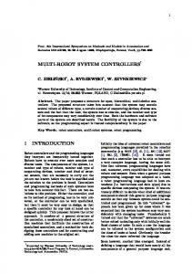
2.1. Mathematical model The control system is assumed to be operating in the linear range. The mathematical model relating the tracking error signal E(z) and the exogenous signals, namely the reference input R(z) and the disturbance W(z), for the plant given in Fig. 1 is

E(z) = [I + SG(z) PC(z)] -l[R(z) - SGw(z) W(z)] where G(z), C(z) and Gw(z) are the plant, controller and disturbance transfer function, R(z) and W(z) are the z-transforms of the reference input and the disturbances, respectively, and P and S represent the actuator and sensor, respectively. It is assumed that R(z) and W(z) are rational polynomials. We define T(z) = [I + SG(z) PC(z)] -1 where T(z) is called the sensitivity function. The H2-norm of T(z) is given by IIT(z)ll2= ~ trace{TT(k) T(k)} = IIT(k)llF2 k=O

where II (.)II~ denotes the Frobenius norm of (.) and T(k) is the impulse weighting sequence (in-

oonl~lgr

actuator

process ~

senso~

Fig. 1. A c o n t r o l s y s t e m c o n s i s t i n g of a process, a c o n t r o l l e r , sensors and actuators.

43

verse z-transform of T(z)). The 2-norm (or H2norm) of T(z) is referred to h e r e i n as the integral squared error (ISE). The vector 0 formed of the n u m e r a t o r and the d e n o m i n a t o r coefficients of T(z) is called the feature vector and it completely characterizes the p e r f o r m a n c e and stability of the control system. Let y(z) be the c o r r u p t e d m e a s u r e m e n t of E(z):

y(z) = s(z) + v(z) where

controller C(z) and the feedback Gw(z), except t h a t the control system is operating in the linear range. These assumptions are less stringent and more realistic in m a n y applications. For example, it is not always possible to k n o w exactly the correct value of the controller p a r a m e t e r s due to zero-offset in the controller p a r a m e t e r knobs and also the exact s t r u c t u r e of the controller m a y be u n k n o w n , for example, say, the i n t e g r a t o r of a PID controller m a y be disconnected [5].

s(z) = T(z) R(z) v(z) = - T(z) SGw(z) W(z) + r(z) s(k) is the t r a c k i n g error signal, r(k) is the meas u r e m e n t noise and v(k) is the corrupting waveform due to disturbance and noise, s(z) is a r a t i o n a l polynomial and has the form s(z)

-

where

b(z) a(z) L

b(z) = ~ bjz -j j-0

L

and

a(z) = 1 -

2 aiz-i i=1

{ai} and {bj} are the autoregressive (AR) and moving-average (MA) coefficients, and L is the order of the system. The class of signals which includes polynomials, damped or growing sinusoids, decaying or growing exponentials and their combinations has a rational z-transform model. This model can be extended to characterize any signal defined on a finite time interval by choosing an a r b i t r a r i l y large order. 2.2. Influence of the control parameters on the feature vector Let ~ be a q × 1 vector, "Y = [°/,, ~2. . . . . 7i . . . . ,7q] ~ formed from the coefficients of the n u m e r a t o r and the d e n o m i n a t o r polynomials of the controller transfer f u n c t i o n C(z). The feature vector 0 is affine in the controller p a r a m e t e r ~, t h a t is, the v a r i a t i o n of 0 is linear in the v a r i a t i o n of the controller p a r a m e t e r 71: A 0 = ~'~i A]2i

w h e r e ~2i is i n d e p e n d e n t of 7- Let ~ = [f2, ~22' • " f2q]. The m a t r i x ~ , which is the Jacobian of the feature vector with respect to the controller p a r a m e t e r vector ~ is called the influence matrix.

2.3. Assumptions No a priori information is assumed on the structure and the p a r a m e t e r s of the plant G(z), the

3. E s t i m a t i o n o f t h e f e a t u r e v e c t o r a n d t h e influence matrix

The vector formed from the n u m e r a t o r and the d e n o m i n a t o r coefficients of the sensitivity function T(z) is termed the feature vector O, and the J a c o b i a n of the feature vector with respect to the physical p a r a m e t e r is the influence matrix. The estimate of the feature vector and the influence matrix form the basis of the proposed perform a n c e monitoring and p e r f o r m a n c e i m p r o v e m e n t scheme. The feature vector is derived from the estimate of the ARMA model of the signal s(k). The estimation of the signal model is a difficult problem since (1) not only the p a r a m e t e r s but also the order of the ARMA model of s(k) v a r y over a large range as the operating conditions c h a n g e and (2) the corrupting waveform v(k) is u n k n o w n , non-stationary and coloured. The signal model is estimated in two stages. In the first stage an ARMA model of the m e a s u r e d error signal is estimated using an LPCA [17, 18], and in the second stage an estimate of the signal model is obtained using a model r e d u c t i o n technique.

3.1. Estimation of the A R M A model The LPCA is a b a t c h least squares algorithm for estimating an ARMA model of the m e a s u r e d signal from a finite n u m b e r of samples { y ( k - i), i = 1, 2 . . . . , N}. It is one of the most reliable, robust and a c c u r a t e methods available [17, 18]. The ARMA model is estimated by minimizing the least square error between the measured signal and the signal predicted from the assumed model: N

min

~ [y(k)-2(k)]2 k=M+l where :~(k) is a one-step prediction ofy(k) based on {y(k - i), i = 1, 2 , . . . , M}, N i s the n u m b e r of samples used to estimate the A R M A model and M is the assumed order of the A R M A model.

44

Because of the assumption of rational spectra, the z-transform of the m e a s u r e d signal is modelled as a rational polynomial and hence the assumed model is given by

2(z) - / ~ (z) ~,,(z) M

~h(Z) ~ - 1 -

M

2 ~hiZ i=1

i,

]~h(Z) :

2 [~hiZ-i i-o

where M is the assumed order, L ~< M ~