Most industrial processes respond to the actions of a feedback controller by moving ... tuning of three-term controllers for SOPD-IR processes (Chen et al, 2005, ...
2 Tuning Three-Term Controllers for Integrating Processes with both Inverse Response and Dead Time K.G. Arvanitis1, N.K. Bekiaris-Liberis2, G.D. Pasgianos1 and A. Pantelous3 1Department
2Department
of Agricultural Engineering, Agricultural Univeristy of Athens, of Mechanical & Aerospace Engineering, University of California-San Diego, 3Department of Mathematical Sciences, University of Liverpool, 1Greece 2USA 3UK
1. Introduction Most industrial processes respond to the actions of a feedback controller by moving the process variable in the same direction as the control effort. However, there are some interesting exceptions where the process variable first drops, then rises after an increase in the control effort. This peculiar behaviour that is well known as “inverse response”, is due to the non-minimum phase zeros appearing in the process transfer function and representing part of the process dynamics. Second order dead-time inverse response process models (SODT-IR) are used to represent the dynamics of several chemical processes (such as level control loops in distillation columns and temperature control loops in chemical reactors), as well as the dynamics of PWM based DC-DC boost converters in industrial electronics. In the extant literature, there is a number of studies regarding the design and tuning of three-term controllers for SOPD-IR processes (Chen et al, 2005, 2006; Chien et al, 2003; Luyben, 2000; Padma Sree & Chidambaram, 2004; Scali & Rachid, 1998; Waller & Nygardas, 1975; Zhang et al, 2000). On the other hand, integrating models with both inverse response and dead-time (IPDT-IR models) was found to be suitable for a variety of engineering processes, encountered in the process industry. The common examples of such processes are chemical reactors, distillation columns and, especially, level control of the boiler steam drum. In recent years, identification and tuning of controllers for such process models has not received the appropriate attention as compared to other types of inverse response processes, although some very interesting results have been reported in the literature (Gu et al, 2006; Luyben, 2003; Shamsuzzoha & Lee, 2006; Srivastava & Verma, 2007). In particular, the method reported by (Luyben, 2003) determines the integral time of a series form PID controller as a fraction of the minimum PI integral time, while the controller proportional gain is obtained by satisfying the specification of +2 dB maximum closed-loop log modulus, and the derivative time is given as the one maximizing the controller gain. In the work proposed by (Gu et al, 2006), PID controller tuning for IPDT-IR processes is performed based on H∞ optimization and Internal Model Control (IMC) theory. In the work
30
PID Controller Design Approaches – Theory, Tuning and Application to Frontier Areas
proposed by (Shamsuzzoha & Lee, 2006), set-point weighted PID controllers are designed on the basis of the IMC theory. Finally, in the work proposed by (Srivastava & Verma, 2007), a method involving numerical integration has been proposed in order to identify process parameters of IPDT-IR process models. From the preceding literature review, it becomes clear that results on controller tuning for IPDT-IR processes are limited, and that there is a need for new efficient tuning methods for such processes. The aim of this work is to present innovative methods of tuning three-term controllers for integrating processes incorporating both time-delay and a non-minimum phase zero. The three-term controller configuration applied in this work is the well known IPD (or Pseudo-Derivative Feedback, PDF) controller configuration (Phelan, 1978) due its advantages over the conventional PID controller configuration (Paraskevopoulos et al, 2004; Arvanitis et al, 2005; Arvanitis et al, 2009a). A series of innovative controller tuning methods is presented in the present work. These methods can be classified in two main categories: (a) methods based on the analysis of the phase margin of the closed-loop system, and (b) methods based on a direct synthesis approach. According to the first class of proposed tuning methods, the controller parameters are selected in order to meet the desired specifications in the time domain, in terms of the damping ratio or by minimizing various integral criteria (Wilton, 1999). In addition, the proportional gain of the controller is chosen in such a way, that the resulting closed-loop system achieves the maximum phase margin for the given specification in the time domain, thus resulting in robust closed-loop performance. Controller parameters are involved in nonlinear equations that are hard to solve analytically. For that reason, iterative algorithms are proposed in order to obtain the optimal controller settings. However, in order to apply the proposed methods in the case of on-line tuning, simple approximations of the exact controller settings obtained by the aforementioned iterative algorithms are proposed, as functions of the process parameters. The second class of proposed tuning methods is based on the manipulation of the closedloop transfer function through appropriate approximations and cancellations, in order to obtain a second order dead-time closed-loop system. On the basis of this method, the parameters of the I-PD controller is obtained in terms of an adjustable parameter that can be further appropriately selected in order either to achieve a desired damping ratio for the closed-loop system or to ensure the minimization of conventional integral criteria. Finally, In order to assess the effectiveness of the proposed control scheme and associated tuning methods and to provide a comparison with existing tuning methods for PID controllers, a simulation study on the problem of controlling a boiler steam drum modelled by an IPDTIR process model is presented. Simulation results reveal that the proposed controller and tuning methods provide considerably smoother response than known design methods for standard PID controllers, in case of set point tracking, as well as lower maximum error in case of regulatory control. This is particular true for the proposed direct synthesis method, which outperforms existing tuning methods for PID controllers.
2. IPDT-IR process models and the I-PD controller configuration This work elaborates on IPDT-IR process models of the form GP ( s )
K s Z 1 exp( ds )
s s p 1
(1)
Tuning Three-Term Controllers for Integrating Processes with both Inverse Response and Dead Time
31
where K , d , P and Z are the process gain, the time delay, the time constant and the zero’s time constant, respectively, controlled using the configuration of Fig. 1, i.e. the socalled I-PD or PDF controller. In this controller configuration, the three controller actions are separated. Integral action, which is dedicated to steady state error elimination, is located in the forward path of the loop, whereas proportional and derivative actions, which are mainly dedicated in assigning the desired closed-loop performance in terms of stability, responsiveness, disturbance attenuation, etc, are located in the feedback path. This separation leads to a better understanding of the role of each particular controller action. Moreover, the I-PD controller has some distinct advantages over the conventional PID controller, as reported in the works by (Paraskevopoulos et al, 2004; Arvanitis et al, 2005; Arvanitis et al, 2009a). Observe now that applying the I-PD control strategy to the process model of the form (1), the following closed-loop transfer function is obtained
GCL (s )
KK I s Z 1 exp( ds )
s P s 1 K K Ds 2 K P s K I 2
s
Z
1 exp( ds )
(2)
It is not difficult to see that the action of the I-PD controller is equivalent to that of a PID controller in series form having the transfer function 1 GC , PID (s ) KC 1 1 Ds Is
(3)
with a second order set-point pre-filter of the form GC ,SPF (s ) 1 / I s 1 1 Ds , provided that the following relations hold
R(s) +
E(s) _
KI s
+ +
L(s) U(s) _
GP(s)
Y(s)
K P K Ds The I-PD control structure Fig. 1. The I-PD or PDF control strategy. K P KC D I / I , K I K P / D I KC / I , K D K P D I / D I KC D
(4)
Taking into account the above equivalence, the loop transfer function of the proposed feedback structure is given by GL ( s )
KKC s Z 1 s 1 Ds 1 exp( ds )
s 2 P s 1
(5)
32
PID Controller Design Approaches – Theory, Tuning and Application to Frontier Areas
Relations (2) and (5) are used in the next Sections for the derivation of the tuning methods proposed in this work.
3. Frequency domain analysis for closed-loop IPDT-IR processes The equivalence between the PD-1F controller and the set-point pre-filtered PID controller provides us the possibility, to work with KC , I and D and not directly with K P , K I and K D . Furthermore, in order to facilitate comparisons, let all system and controller parameters be normalized with respect to P and K . Thus, the original process and controller parameters are replaced with the dimensionless parameters shown in Table 1. Then, relations (2) and (5) yield
GCL (sˆ )
KC sˆ Z 1 exp( dsˆ )
(6)
I s sˆ 1 KC sˆ 1 Dsˆ 1 sˆ Z 1 exp( dsˆ ) ˆ2
GL ( sˆ )
KC sˆ Z 1 sˆ 1 Dsˆ 1 exp( dsˆ )
(7)
sˆ 2 sˆ 1
From relation (7), the argument and the magnitude of the loop transfer function are given by
φL(w)= -π – dw - atan(w) - atan(τZw) + atan(τIw) + atan(τDw) Original Parameters
(8)
Normalized Parameters
Original Parameters
τp=1
S
Normalized Parameters sˆ s P
Z
Z Z / P
K
Κ=1
d
d d / P
KC
KC KKC
I / P
KD
KD KKD
D
D D / P
KP
K P p KK P
ω
w P
KI
K I p2 KK I
p
Table 1. Normalized vs. original system parameters. AL w GL jw KC
1 w
2
1 D w
2
w2 1 w2
1 Z w
2
(9)
In Fig. 2, the Nyquist plots of GL(ŝ) for typical IPDT-IR processes are depicted for several values of the parameter τΙ. From this figure, it becomes clear that, for specific d and τΖ, and for τΙ greater than a critical value, say τΙ,min, there exists a crossover point of the Nyquist plot with the negative real axis. In this case, the system can be stabilized, with an appropriate choice of KC. Moreover, from these Nyquist plots, one can observe that the stability region is reduced when τΙ is decreased, starting from the maximum region of stability when τΙ , (which corresponds to a PD-controller). The Nyquist plot does not have any crossover point
Tuning Three-Term Controllers for Integrating Processes with both Inverse Response and Dead Time
33
with the negative real axis, in the case where τΙ=τΙ,min; that is, for τΙτΙ,min, the process cannot be stabilized. Moreover, in Fig. 3, the Nyquist plots of GL(ŝ) are depicted for several values of the parameter τD. From these plots, it becomes clear that, for small values of τD, the stability region is increased with τD, whereas for larger values of τD the stability region decreases when τD increases. Let PM=φ(wG)+π be the phase margin of the closed-loop system, where wG is the frequency, at which the magnitude of the loop transfer function GL(ŝ) equals unity. Taking into account (8), we obtain PM = -dwG – atan(wG) - atan(τZwG) + atan(τIwG) + atan(τDwG). From Fig. 2, it can be readily observed that for given d, τΙ, τD, τZ, there exists one point of the Nyquist plot corresponding to the maximum argument φL,max(d, τΙ, τD, τΖ). The frequency wP at which the argument (8) is maximized is given by the maximum real root of the equation dL w / dw 0 , which, after some easy algebraic manipulations, yields w wP
d
1 1 wP 2
Z
1 Z 2 wP 2
1 2 wP 2
D
1 D2 wP 2
0
(10)
Hence, substituting wP, as obtained by (10), in (8), the respective argument φL(wP) is computed. Consequently, the maximum phase margin PMmax for given d, τΙ, τD, τΖ, can be obtained if we put wP=wG, i.e. choosing the controller proportional gain ΚC according to KC
I wP 2 1 wP 2 1 D wP
2
1 I wP
2
1 Z wP
2
(11)
With this choice for KC, the phase margin is given by PM d , I , D , Z dwP a tan wP a tan Z wP
a tan I wP a tan D wP PMmax d , I , D , Z
(12)
Obviously, in the case where τΙ=τΙ,min and KC is obtained by (11), then the closed-loop system is marginally stable, that is PMmax=0. Note that, from (12), PMmax=0, when wP=0. Therefore, from (10), for wP=0, we obtain τΙ,min=d+τΖ+1-τD. Since, for all values of τΙ, larger than τΙ,min=d+τΖ+1-τD, it holds
d PM d , I , D , Z / dw w0 =τΙ+τD-d-τΖ-1>0,
one can readily
conclude that PMmax>0. Moreover, PMmax is an increasing function of both τΙ and τD. This is illustrated in Fig. 4, where PMmax is given as a function of τΙ and τD, for a typical IPDT-IR process. As it was previously mentioned, the stability region of the closed-loop system increases with τD. This is due to the fact that the closed-loop system gain margin increases with τD, as one can verify from the variation of the crossover point of the Nyquist plot with the negative real axis as τD varies. Furthermore, there is one value of τD, say D ,GMmax (τ I , τ Z ,d) , for which the closed loop gain margin starts to decrease. In addition, from Fig. 2, it can be easily verified that the closed-loop gain margin increases arbitrarily as τI increases. These observations can also become evident from Fig. 5 that illustrates the maximum closed-loop gain margin GMmax as a function of the controller parameters τD and τI.
34
PID Controller Design Approaches – Theory, Tuning and Application to Frontier Areas 0.6
I= I,min=0.5
0.4 0.2 0 PMmax
Imaginary
-0.2 -0.4
I=1.5
-0.6
I=2.5
-0.8 -1
I=5 -1.2 -1.4 -2
-1.5
-1
-0.5
0
Real
Fig. 2. Nyquist plots of a typical IPDT-IR process controlled by a PD1-F controller with KC=0.5, d=0.5, τΖ=0.5, τD=1.5, for various values of τΙ.
0.1 0
D=0.2
Imaginary
-0.1 -0.2
D=0.4 -0.3
D= DmaxGM(I,d,Z)=0.874 -0.4 -0.5
D=1.1
-0.6 -1.8
-1.6
-1.4
-1.2
-1
-0.8 Real
-0.6
-0.4
-0.2
0
Fig. 3. Nyquist plots of a typical IPDT-IR process controlled by a PD-1F controller with KC=0.3, d=0.5, τΖ=0.5, τI=2.5, for various values of τD.
Tuning Three-Term Controllers for Integrating Processes with both Inverse Response and Dead Time
35
It can also be observed, from Fig. 5, that the value of D ,GMmax (τ I , τ Z ,d) decreases as τI increases and it takes its minimum value, denoted by min D ,GMmax (τ Z ,d) , when τI. This is also evident from Fig. 6, where D ,GMmax (τ I , τ Z ,d) is depicted, as a function of τI, for several values of τΖ and d. Applying optimization techniques using MATLAB®, it is plausible to provide accurate approximations of that limit as a function of the normalized parameters d and τΖ. These approximations are summarized in Table 2. Note that, the maximum normalized error (M.N.E.), defined by min ˆD,GM ( Z , d )-min D,GM ( Z , d ) max max max , where min ˆD ,GMmax ( Z , d ) min D ,GMmax ( Z , d ) denotes the approximate value, never exceeds 3%, for a wide range of d and τZ. Finally, another interesting value relative to τD, is τD,maxGM,I-P(τI,τD,d) that denotes the maximum value of τD, for which the gain margin obtained by an I-PD controller is larger than the gain margin obtained by an I-P controller. It is worth noticing that the value of τD,maxGM,I-P(τI,τD,d) decreases as τΙ increases and it takes its minimum value, which is denoted by minτD,maxGM,I-P(τI,τD,d), when τΙ. This is evident from Fig. 7, which illustrates τD,maxGM,IP(τI,τD,d) as a function of τΙ, for several pairs (τΖ,d). Application of optimization techniques yields some useful approximations of this parameter, which are summarized in Table 3. These approximations are quite accurate, since the respective maximum normalized errors never exceed 5%, for a wide range of d and τZ.
4. Controller tuning based on the maximum phase margin specification The above analysis provides us the means to propose an efficient method for tuning I-PD controllers for IPDT-IR processes. The main characteristic of the proposed tuning method, which is designated as Method I in the sequel, is the selection of the controller gain KC using (11). The remaining two parameters τΙ and τD can be selected such that a specific closed-loop performance is achieved. In particular, one can select the parameter τΙ in order to achieve a specific closed-loop response while selecting the parameter τD in order to improve this response in terms of the achievable gain margin or in terms of the minimization of several integral criteria, such as the well-known ISE criterion, the integral of squared error plus the normalized squared controller output deviation from its final value u (ISENSCOD criterion) of the form J ISENSCOD
0
y(t) r(t)
2
K 2 u(t ) u dt 2
(13)
or the integral of squared error plus the normalized squared derivative of the controller output (ISENSDCO criterion), having the form J ISENSDCO
0
y(t) r(t)
2
K 2 p2 u (t )2 dt
(14)
36
PID Controller Design Approaches – Theory, Tuning and Application to Frontier Areas
0.8
0.6 PMmax 0.4 0.2
0 1 0.5
D 0
2
0
8
6
4
10
I
Fig. 4. PMmax as a function of τI and τD for a typical IPDT-IR with d=τZ=1.5.
1.5
1 GMmax 0.5
0 1.5
6 4
1
D
2
0.5 0
0
I
Fig. 5. GMmax as a function of τI and τD for a typical IPDT-IR process with d=τZ=0.5.
Tuning Three-Term Controllers for Integrating Processes with both Inverse Response and Dead Time
37
2.4 2.2 2 1.8 D,GMmax I , Z ,d 1.6
1.4 1.2
Z ,d 1.5,1.5
1 0.8 0.6 0.4 0
Z ,d 0.5,1.5
Z ,d 1.5,0.5
Z ,d 0.5,0.5 10
20
30
40
50 I
60
70
80
90
100
Fig. 6. Parameter D ,GMmax ( I , Z , d ) as a function of τI, for several values of τZ and d. minτD,GMmax(d,τΖ) -0.0561+0.555d-0.0629τΖ2+0.1308τΖ-0.372d2-0.1171(d+τΖ)3+0.5144(d+τΖ)0.5 for 0